CP asymmetry in $B\to\phi K_{S}$ in a SUSY SO(10) GUT

Abstract

We study the $B\to\phi K_{S}$ decay in a SUSY SO(10) GUT. We calculate the mass spectrum of sparticles for a given set of parameters at the GUT scale. We complete the calculations of the Wilson coefficients of operators including the new operators which are induced by NHB penguins at LO using the MIA with double insertions. It is shown that the recent experimental results on the time-dependent CP asymmetry $S_{\phi K}$ in $B\to\phi K_{S}$, which is negative and can not be explained in SM, can be explained in the model where there are flavor non-diagonal right-handed down squark mass matrix elements of 2nd and 3rd generations whose size satisfies all relevant constraints from known experiments ($\tau\to\mu\gamma$, $B\to X_{S}\gamma,B_{s}\to\mu^{+}\mu^{-},B\to X_{s}\mu^{+}\mu^{-},B\to X_{s}g,\Delta M_{s}$, etc.). At the same time, the branching ratio for the decay can also be in agreement with experimental measurements.

I Introduction

Great progresses have been made on the flavor physics in recent years. Among them the progress in neutrino physics is particularly impressive. Atmospheric neutrino skatm and solar neutrino sno experiments together with the reactor neutrino kamland ; chooz experiments have established the oscillation solution to the solar and atmospheric neutrino anomalies, which signals the existence of new physics beyond the SM. Experiment results indicate smallness of the masses of neutrinos and the bilarge mixing pattern among the three generations of neutrinos. Because the small quark mixing in the CKM matrix is related to the large quark mass hierarchy wwzf , understanding the bilarge mixing pattern is somewhat of a challenge. However, if allowing asymmetric form for the mass matrix which for example may well be generated by the elegant Froggatt-Nielsen (FN) mechanism FN , we can accommodate the large mass hierarchy with large mixing asy . Therefore, if one works with an effective theory, e.g., the minimal supersymmetric Standard Model together with right-hand neutrinos (MSSM+N), at a low energy scale (say, the electro-weak scale), one can content oneself by using the WWZF scenario to understand the smallness of quark mixing, and the see-saw and FN mechanism to understand the smallness of the masses of neutrinos and the largeness of neutrino mixing. However, if one works with a theory, e.g., a grand unification theory (GUT), in which quarks and leptons are in a GUT multiplet, one has to answer: can we explain simultaneously the smallness of quark mixing and the largeness of neutrino mixing in the theory? If we can, then what are the phenomenological consequences in the theory? There are several recent works to tackle these problems in SU(5), flipped SU(5), or SO(10) GUTs  asy ; bdv ; lfv3 ; cmm ; mvv ; bsv ; hs ; hll , which brings the study of GUT to a more realistic level.

The smallest grand unification group that incorporates righthanded neutrinos required for the seesaw mechanism, is SO(10). It has been shown that the observed bilarge mixing naturally leads to large flavor non-diagonal down-type squark mass matrix elements of 2nd and 3rd generations in a SUSY SO(10) cmm .

The measurements of the time dependent CP asymmetry $S_{J/\psi K}$ in $B\to J/\psi K_{S}$ have established the presentence of CP violation in neutral B meson decays and the measured valuesj

$$S_{J/\psi K}=\sin(2\beta(J/\psi K_{S}))_{\rm world-ave}=0.734\pm 0.054.$$ (1)

is in agreement with the prediction in the standard model (SM). Recently, various measurements of CP violation in B factory experiments have attracted much interest. Among them2002 ; 2003 ,

$$S_{\phi K_{S}} = -0.39\pm 0.41,\,\,\,\,\,2002\,\,\,{\rm World-average}$$

$$S_{\phi K_{S}} = -0.15\pm 0.33,\,\,\,\,\,2003\,\,\,{\rm World-average}$$ (2)

is especially interesting since it deviates greatly from the SM expectation

$$S_{\phi K_{S}}=\sin(2\beta(\phi K_{S}))=\sin(2\beta(J/\psi K_{S})\!)\!+\!O(\lambda^{2}\!)$$ (3)

where $\lambda\simeq 0.2$ appears in Wolfenstein’s parameterization of the CKM matrix. Though the impact of these experimental results on the validity of CKM and SM is currently limited by experimental uncertainties, they have attracted much interest in searching for new physics dat ; kk ; kane ; chw ; hz and it has been shown that the deviation can be understood without contradicting the smallness of the SUSY effect on $B\to J/\psi K_{S}$ in the minimal supersymmetric standard model (MSSM) kane ; chw . Motivated by SUSY GUTs, the time dependent CP asymmetry in $B\to\phi K_{S}$ has been studied in the SUSY models with a large mixing between the 2nd and 3rd generation in the down-type squark mass matrix at the $M_{SUSY}\sim TeV$ scale hlm . The asymmetry has also been examined in the SUSY SU(5) framework cmsvv . It is shown in ref. cmsvv that the possibility of large deviations from SM in $S_{\phi K}$ is excluded in the case of only having the flavor non-diagonal down-type squark mass matrix element of 2nd and 3rd generations in the RR sector (i.e., $\delta_{23}^{dRR}$ non-zero with $\delta_{23}^{dRR}\equiv(M^{2}_{\tilde{d}RR})_{23}/m_{\tilde{q}}^{2}$, where $(M^{2}_{\tilde{d}RR})_{ij}$ is the flavor non-diagonal squared right-handed down squark mass matrix element and $m_{\tilde{q}}$ is the average right-handed down-type squark mass) due to the bound on $\delta_{23}^{dRR}$ from $Br(\tau\to\mu\gamma)$. In this paper we investigate the decay $B\to\phi K_{S}$ in the SUSY SO(10) framework. Our results show that the time dependent CP asymmetry in $B\to\phi K_{S}$ can sizably deviate from SM after imposing the constraint from $Br(\tau\to\mu\gamma)$, in contrast with the claim in the literature, because we have included the double insertion contributions in penguin diagrams for the relevant Wilson coefficients. Furthermore, the contributions from neutral Higgs penguins, which are not considered in ref. cmsvv , have been included in this paper.

We need to have new CP violation sources in addition to that of CKM matrix in order to explain the deviations of $S_{\phi K_{S}}$ from SM. There are new sources of flavor and CP violation in SUSY SO(10) GUTs. In such kind of models there is a complex flavor non-diagonal down-type squark mass matrix element of 2nd and 3rd generations of order one at the GUT scale cmm which can induce large flavor off-diagonal couplings such as the coupling of gluino to the quark and squark which belong to different generations. These couplings are in general complex and consequently can induce CP violation in flavor changing neutral currents (FCNC). It is well-known that the effects of the counterparts of usual chromo-magnetic and electro-magnetic dipole moment operators with opposite chirality are suppressed by ${m_{s}}/{m_{b}}$ and consequently negligible in SM. However, in SUSY SO(10) GUTs their effects can be significant, since $\delta_{23}^{dRR}$ can be as large as 0.5 cmm .

For the $b\to s$ transition, besides the SM contribution, there are mainly two new contributions arising from the QCD and chromo-magnetic penguins and neutral Higgs boson (NHB) penguins with the sparticles propagating in the loop in SUSY models. The contributions to the relevant Wilson coefficients at the $m_{W}$ scale from the diagram with the gluino propagating in the loop have been calculated by using the mass insertion approximation (MIA) mi with double insertions in ref. chw . We calculate the contributions from the diagram with the chargino propagating in the loop using MIA with double insertions because chargino contributions can be significant when the left-right mixing between squark masses is large.

As it is shown that both Br and CP asymmetries depend significantly on how to calculate hadronic matrix elements of local operatorschw . Recently, two groups, Li et al. li1 ; li and BBNS bbns ; bbns1 , have made significant progress in calculating hadronic matrix elements of local operators relevant to charmless two-body nonleptonic decays of B mesons in the PQCD framework. The key point to apply PQCD is to prove that the factorization, the separation of the short-distance dynamics and long-distance dynamics, can be performed for those hadronic matrix elements. It has been shown that in the heavy quark limit (i.e., $m_{b}\to\infty$) such a separation is indeed valid and hadronic matrix elements can be expanded in $\alpha_{s}$ such that the tree level (i.e., the $\alpha_{s}^{0}$ order) is the same as that in the naive factorization and the $\alpha_{s}$ corrections can be systematically calculatedbbns . Comparing with the naive factorization, to include the $\alpha_{s}$ correction decreases significantly the hadronic uncertainties. In particular, the matrix elements of the chromomagnetic-dipole operators $Q_{8g}^{(\prime)}$ have large uncertainties in the naive factorization calculation which lead to the significant uncertainty of the time dependent CP asymmetry in SUSY modelshlm . The uncertainties are greatly decreased in BBNS approachbbns1 . The hadronic matrix element of operators relevant to the decays $B\rightarrow\phi K_{S}$ up to the $\alpha_{s}$ order have been calculated in BBNS approach in ref. chw .

Using the BBNS approach to calculate hadronic elements to the $\alpha_{s}$ order and Wilson coefficients in MIA with double insertions, we show in this paper that in the SUSY $SO(10)$ framework in the reasonable region of parameters where the constraints from $\tau\to\mu\gamma$, $B_{s}-\bar{B}_{s}$ mixing , $\Gamma(b\to s\gamma)$, $\Gamma(b\to sg)$, $\Gamma(b\to s\mu^{+}\mu^{-})$, and $B\to\mu^{+}\mu^{-}$ are satisfied, the branching ratio of the decay for $B\rightarrow\phi K_{S}$ can be smaller than $1.6\times 10^{-5}$, and the theoretical prediction for $S_{\phi K}$ can be in agreement with the data in $1\sigma$ experimental bounds and even can be as low as $-0.6$.

The paper is organized as follows. In Section II we describe the SO(10) models we used in the paper briefly. In section III we calculate sparticle spectrum using revised ISAJET. In section IV we give the effective Hamiltonian responsible for $B\rightarrow\phi K_{S}$ in the model. In particular, we give the Wilson coefficients of operators using MIA with double insertions. The Section V is devoted to numerical results of the time dependent CP asymmetry and branching ratio for the decay $B\to\phi K_{S}$. We draw conclusions and discussions in Section VI.

II Neutrino Bilarge Mixing and large b-s transitions in SO(10)GUT

It is well-known for a long time that SO(10) GUTs can naturally incorporate the seesaw mechanism seesaw which is the simplest way to understand small neutrino masses. Recently a number of SUSY SO(10) models which can explain neutrino data and quark mixing have been proposed asy ; cmm ; bsv and some phenomenological consequences of the models have been analyzed asy ; bi ; cmm . It was first pointed out in  cmm that the induced large mixing in the down-type squark mass matrix in SUSY $SO(10)$ models have interesting consequences in low energy B physics. For specific, we use the model in ref. cmm and review the main points of the model. The details of the model can be found in Ref. cmm .

In order to accommodate both CKM mixing among quarks and MNS mixing among leptons, one needs to have an asymmetric down-type Yukawa matrix $Y_{d}$. So instead of the usual superpotential dh , one assumes

$$W=\frac{1}{2}(Y_{u})_{ij}16_{i}16_{j}10_{u}+\frac{1}{2}(Y_{d})_{ij}16_{i}16_{j}\frac{\langle 45\rangle}{M_{Pl}}10_{d}.$$ (4)

Because of the combination of the Higgs multiplet $45$, whose VEV $\langle 45\rangle\neq 0$ breaks SO(10), and the Higgs in 10, the effective Yukawa coupling being either in 10 (symmetric between two 16’s) or 120 (anti-symmetric between two 16’s) representations, the matrix $Y_{d}$ can now have a mixed symmetry. Setting the breaking chain to be $SO(10)\to SU(5)\to SM$, we have the Yukawa couplings in the MSSM+N (the MSSM with right-handed neutrinos) as

$$W=(Y_{u}^{D})_{i}Q_{i}U_{i}H_{u}+(Y_{u}^{D})_{i}L_{i}N_{i}H_{u}$$ (5)

$$+(V^{*}Y_{d}^{D}U)_{ij}Q_{i}D_{j}H_{d}+(V^{*}Y_{d}^{D}U)_{ij}E_{i}L_{j}H_{d}+\frac{1}{2}M_{ij}N_{i}N_{j},$$

where $Y_{i}^{D}$ (i=u, d) is the diagonal and we have absorbed the phase matrix $\Theta_{L}$ into $Q_{i}$ and $E_{i}$, the phase matrix $\Theta_{R}$ into $(UD)$ multiplet or $(EV^{*})$ multiplet, and the phase matrix $\Theta_{\nu}$ into the Majorana mass matrix $M$, respectively. Here V and U are the usual CKM mixing matrix and neutrino mixing matrix (MNS matrix) respectively. We have taken $Y_{u}$ and $M$ simultaneously diagonal. Such a situation could result from simple $U(1)$ family symmetries and in a $SO(10)$ with hierarchical $Y_{u}^{D}$ and right-handed neutrino masses, the choice of having such simultaneous diagonalization looks rather plausible bw .

After integrating out the right-handed neutrinos in Eq. (5), the light neutrino masses are determined from the superpotential

$$W=\frac{1}{2}(Y_{u}^{D})_{i}(M^{-1})_{ij}(Y_{u}^{D})_{j}(L_{i}H_{u})(L_{j}H_{u}),$$ (6)

which leads to the light Majorana neutrino mass matrix $(m_{\nu})_{nm}=(Y_{ui}^{D2}/2M_{i})U_{ni}^{*}e^{-i\delta_{i}}U_{mi}^{*}$, where $e^{i\delta_{i}}$ is the phase of the diagonal element $M_{i}$ of the diagonal matrix M. Therefore, the two mass splitting data and bilarge mixing of neutrinos can be explained.

The Yukawa coupling of “third-generation” neutrino is unified with the large top Yukawa coupling due to the $SO(10)$ unification. Nevertheless, this “third-generation” neutrino is actually a near-maximal mixture of $\nu_{\mu}$ and $\nu_{\tau}$, which comes from the large mixing angle in atmospheric neutrino oscillation. Because the “third-generation” charged leptons, down-type quarks and neutrinos are in a $SU(5)$ multiplet, the $SU(5)$ multiplet with the large top Yukawa coupling contains approximately

$$5^{*}_{3}=5^{*}_{\tau}\cos\theta+5^{*}_{\mu}\sin\theta,$$ (7)

where $\theta\simeq 45^{\circ}$ is the atmospheric neutrino mixing angle, and

$$5^{*}_{\tau} = (b^{c},b^{c},b^{c},\nu_{\tau},\tau)$$ (8)

$$5^{*}_{\mu} = (s^{c},s^{c},s^{c},\nu_{\mu},\mu).$$ (9)

The similar mixing exists in right-handed b and s quarks. However, we do not worry about its effects because there is no charged-current weak interaction on right-handed quarks. Therefore the mixing among right-handed quarks decouples from low-energy physics.

We now come to the main outcome in the framework which has phenomenological consequences in low-energy B physics. Because one works in SUSY models there is the corresponding mixing among squarks which would yield observable effects. The top Yukawa coupling generates an $O(1)$ radiative correction to the mass of $\tilde{s}\sin\theta+\tilde{b}\cos\theta$, which leads to a large mixing between $\tilde{s}$ and $\tilde{b}$ at low energies. This large mixing in turn generates interesting effects in $B$-physics.

To be specific, assuming that at the scale $M_{*}$ which is above the GUT unification scale, say, near the Planck scale, one has the universal soft terms: scalar mass $m_{0}$, gaugino mass $M_{1/2}$, trilinear and bilinear couplings $A_{0}$ and $B_{0}$, then large neutrino Yukawa couplings involved in the neutrino Dirac masses can induce large off-diagonal mixing in the right-handed down squark mass matrix through renormalization group evolution between $M_{*}$ and $M_{GUT}$ and the induced mixings will generally be complex with new CP violating phases. The induced off-diagonal elements in the mass matrix of the right-handed down squarks $\tilde{d}_{R}$ are given by (in the basis in which $Y_{D}$ is diagonal)

$$[m^{2}_{\tilde{d}_{R}}]_{nm}\simeq-\frac{1}{8\pi^{2}}\left[Y^{u\dagger}Y^{u}\right]_{nm}(3m_{0}^{2}+a_{0}^{2})\left(5\log\frac{M_{*}}{M_{10}}+\log\frac{M_{10}}{M_{5}}\right)$$ (10)

where $M_{5}$ is the $SU(5)$ breaking scale and

$$\left[Y^{u\dagger}Y^{u}\right]_{nm}=\left[(\Theta_{R}UY_{u}^{D2}U^{\dagger}\Theta_{R}^{*}\right]_{nm}=e^{-i(\phi^{(L)}_{m}-\phi^{(L)}_{n})}y_{t}^{2}\left[U\right]_{m3}^{*}\left[U\right]_{n3},$$ (11)

where $e^{i\phi^{(L)}_{n}}$ is the phase from $(\Theta_{R})_{nn}$. Note that these phases are not relevant to any other low energy physics.

Substituting $U_{23,33}\sim\sqrt{2}$ into eq.(11), one obtains

$$[Y^{u\dagger}Y^{u}]_{23}=0.5e^{-i(\phi^{(L)}_{2}-\phi^{(L)}_{3})}(m_{t}(M_{G})/178\mbox{ GeV})^{2},$$ (12)

where $m_{t}(M_{G})$ is the top quark mass at $M_{G}$. From eqs. (10,12), the mass insertion parameter $\delta^{dRR}_{23}$ can easily be of order one.

III Mass spectra and the permitted parameter space

To see the impact of the induced off-diagonal elements in the mass matrix of the right-handed down-type squarks on B rare decays and simplify the analysis, we assume that at the GUT scale ($M_{G}$) all sfermion mass matrices except the right-handed down-type squark mass matrix are flavor diagonal and all diagonal elements are approximately universal and equal to $m^{2}_{0}$. The 2-3 matrix element of right-handed down-type squark mass matrix is parameterized by $\delta_{23}^{dRR}\equiv(M^{2}_{\tilde{d}RR})_{23}/m_{0}^{2}$ which can be treated as a free parameter of order one, as discussed in last section. Furthermore, we have a universal gaugino mass $M_{1/2}$, a universal trilinear coupling $A_{0}$ and a universal bilinear coupling $B_{0}$ at $M_{G}$. With the requirement of radiative electro-weak (EW) symmetry breaking, we have five parameters ($m_{0},M_{1/2},A_{0},\delta_{23}^{dRR},tan\beta$) plus the sign of $\mu$ as the initial conditions for solving the renormalization group equations (RGEs).

We require that the lightest neutralino be the lightest supersymmetric particle (LSP) and use several experimental limits to constraint the parameter space, including 1)the width of the decay $Z\rightarrow\chi^{0}_{1}\chi^{0}_{1}$ is less than 4.3 MeV, and branching ratios of $Z\rightarrow\chi^{0}_{1}\chi^{0}_{2}$ and $Z\rightarrow\chi^{0}_{2}\chi^{0}_{2}$ are less than $1\times 10^{-5}$, where $\chi^{0}_{1}$ is the lightest neutralino and $\chi^{0}_{2}$ is the other neutralino, 2) the mass of light neutral even Higgs can not be lower than 111 GeV as the present experments required, 3) the mass of lighter chargino must be larger than 94 GeV as given by the Particle Data Group pdg , 4) sneutrinos are larger than 94GeV, 5) seletrons are larger than 73GeV, 6) smuons larger than 94 GeV, 7) staus larger than 81.9 GeV.

We use revised ISAJET to do numerical calculations. We find that the parameter $(M^{2}_{\tilde{d}RR})_{23}$ does not receive any significant correction and the diagonal entries are significantly corrected, which is in agreement with the results in ref. cmsvv . We scan $m_{0},\;M_{1/2}$ in the range (100, 800) GeV for given values of $A_{0},\tan\beta$ and sign($\mu$)=+1 We impose the constraints from the relevant low energy experiments such as $B\to X_{s}\gamma$, etc. (for the detailed analysis of the constraints, see section V).

As an illustration, the mass spectra without and with the constraints from the low energy experiments are given in Fig. 1 and 2, respectively, where (a) and (b) are for $A_{0}=0,-1000$GeV respectively. Fig. 1 is plotted for $M_{1/2}=200GeV,\tan\beta=40$ and Fig. 2 for $M_{1/2}=500GeV,\tan\beta=40$. One can see from the Figs. 1, 2 that the mass spectrum lifts when $|A_{0}|$ decreases. When the constraints from the low energy experiments are imposed, some mass spectra are excluded and for the allowed spectra the masses of sparticles are similar to those without the constraints.

Figure 1: The mass spectrum versus $m_{0}$ for fixed $M_{1/2}$=200GeV, $\tan\beta$=40, $\delta^{d}_{23RR}=(0.12+0.03i)$, and sign($\mu$)=+1 without the constraints from the low energy experiments imposed. (a) is for $A_{0}=0$. (b) is for $A_{0}$=-1000GeV.

Figure 2: The mass spectrum versus $m_{0}$ for fixed $M_{1/2}$=500GeV, $\tan\beta$=40, $\delta^{d}_{23RR}=(0.12+0.03i)$, and sign($\mu$)=+1 with the constraints from the low energy experiments imposed. (a) is for $A_{0}=0$. (b) is for $A_{0}$=-1000GeV.

IV Effective Hamiltonian for $b\rightarrow s$ transition

The effective Hamiltonian for $b\rightarrow s$ transition can be expressed asbur ; chw

$${\cal H}_{\rm eff} = \frac{G_{F}}{\sqrt{2}}\sum_{p=u,c}\!V_{pb}V^{*}_{ps}\bigg{(}C_{1}\,Q_{1}^{p}+C_{2}\,Q_{2}^{p}+\!\sum_{i=3,\dots,16}\![C_{i}\,Q_{i}+C_{i}^{\prime}\,Q_{i}^{\prime}]$$ (13)

$$+C_{7\gamma}\,Q_{7\gamma}+C_{8g}\,Q_{8g}+C_{7\gamma}^{\prime}\,Q_{7\gamma}^{\prime}+C_{8g}^{\prime}\,Q_{8g}^{\prime}\,\bigg{)}+\mbox{h.c.}\,$$

Here $Q_{i}$ are quark and gluon operators and are given by

$$Q_{1}^{p}=(\bar{s}_{\alpha}p_{\beta})_{V-A}(\bar{p}_{\beta}b_{\alpha})_{V-A},\hskip 65.44142ptQ_{2}^{p}=(\bar{s}_{\alpha}p_{\alpha})_{V-A}(\bar{p}_{\beta}b_{\beta})_{V-A},$$

$$Q_{3(5)}=(\bar{s}_{\alpha}b_{\alpha})_{V-A}\sum_{q}(\bar{q}_{\beta}q_{\beta})_{V-(+)A},\hskip 28.45274ptQ_{4(6)}=(\bar{s}_{\alpha}b_{\beta})_{V-A}\sum_{q}(\bar{q}_{\beta}q_{\alpha})_{V-(+)A},$$

$$Q_{7(9)}={3\over 2}(\bar{s}_{\alpha}b_{\alpha})_{V-A}\sum_{q}e_{q}(\bar{q}_{\beta}q_{\beta})_{V+(-)A},\hskip 11.38092ptQ_{8(10)}={3\over 2}(\bar{s}_{\alpha}b_{\beta})_{V-A}\sum_{q}e_{q}(\bar{q}_{\beta}q_{\alpha})_{V+(-)A},$$

$$Q_{11(13)}=(\bar{s}\,b)_{S+P}\sum_{q}\,{m_{q}\over m_{b}}(\bar{q}\,q)_{S-(+)P}\,,$$

$$Q_{12(14)}=(\bar{s}_{i}\,b_{j})_{S+P}\sum_{q}\,{m_{q}\over m_{b}}(\bar{q}_{j}\,q_{i})_{S-(+)P}\,,$$

$$Q_{15}=\bar{s}\,\sigma^{\mu\nu}(1+\gamma_{5})\,b\sum_{q}\,{m_{q}\over m_{b}}\bar{q}\,\sigma_{\mu\nu}(1+\gamma_{5})\,q\,,$$

$$Q_{16}=\bar{s}_{i}\,\sigma^{\mu\nu}(1+\gamma_{5})\,b_{j}\sum_{q}\,{m_{q}\over m_{b}}\bar{q}_{j}\,\sigma_{\mu\nu}(1+\gamma_{5})\,q_{i}\,,$$

$$Q_{7\gamma}={e\over 8\pi^{2}}m_{b}\bar{s}_{\alpha}\sigma^{\mu\nu}F_{\mu\nu}(1+\gamma_{5})b_{\beta},$$

$$Q_{8g}={g_{s}\over 8\pi^{2}}m_{b}\bar{s}_{\alpha}\sigma^{\mu\nu}G_{\mu\nu}^{a}{\lambda_{a}^{\alpha\beta}\over 2}(1+\gamma_{5})b_{\beta},$$ (14)

where $(\bar{q}_{1}q_{2})_{V\pm A}=\bar{q}_{1}\gamma^{\mu}(1\pm\gamma_{5})q_{2}$, $(\bar{q}_{1}q_{2})_{S\pm P}=\bar{q}_{1}(1\pm\gamma_{5})q_{2}$ , $p=u,c$, $q=u,d,s,c,b$, $e_{q}$ is the electric charge number of $q$ quark, $\lambda_{a}$ is the color SU(3) Gell-Mann matrix, $\alpha$ and $\beta$ are color indices, and $F_{\mu\nu}$ ($G_{\mu\nu}$) are the photon (gluon) fields strength.

The primed operators, the counterpart of the unprimed operators, are obtained by replacing the chiralities in the corresponding unprimed operators with opposite ones. The SUSY contributions to Wilson coefficients have been calculated by using the vertex method in ref. hw . The SUSY contributions due to gluino box and penguin diagrams to the relevant Wilson coefficients at the $m_{W}$ scale in MIA with double insertions, as investigated in ref everett01 , which are non-negligible if the mixing between left-handed and right-handed sbottoms is large have been given in refs.hw ; chw1 . We calculate the chargino contributions in MIA with double insertions and results are

$$C_{3} = \frac{1}{48}\frac{\alpha_{s}}{4\pi}\frac{m^{2}_{w}}{m^{2}_{\tilde{\chi}^{\pm}_{i}}}[\frac{K^{\ast}_{22}}{K^{\ast}_{32}}V_{i1}V^{\ast}_{i1}(F_{6}(x)\delta^{uLL}_{23}+F^{\prime}_{6}(x)\delta^{uLR}_{23}\delta^{uLR}_{33})$$

$$-\frac{K^{\ast}_{22}}{K^{\ast}_{32}}V_{i1}V^{\ast}_{i2}h_{t}(F_{6}(x)\delta^{uLR}_{23}+F^{\prime}_{6}(x)\delta^{uLL}_{23}\delta^{uLR}_{33})$$

$$-2V_{i1}V^{\ast}_{i2}h_{t}F_{6}(x)\delta^{uLR}_{33}]$$

$$C_{4} = -\frac{1}{144}\frac{\alpha_{s}}{4\pi}\frac{m^{2}_{w}}{m^{2}_{\tilde{\chi}^{\pm}_{i}}}[\frac{K^{\ast}_{22}}{K^{\ast}_{32}}V_{i1}V^{\ast}_{i1}(F_{6}(x)\delta^{uLL}_{23}+F^{\prime}_{6}(x)\delta^{uLR}_{23}\delta^{uLR}_{33})$$

$$-\frac{K^{\ast}_{22}}{K^{\ast}_{32}}V_{i1}V^{\ast}_{i2}h_{t}(F_{6}(x)\delta^{uLR}_{23}+F^{\prime}_{6}(x)\delta^{uLL}_{23}\delta^{uLR}_{33})$$

$$-2V_{i1}V^{\ast}_{i2}h_{t}F_{6}(x)\delta^{uLR}_{33}]$$

$$C_{5} = C_{3}$$

$$C_{6} = C_{4}$$

$$C_{7\gamma} = \frac{1}{72}\frac{m^{2}_{w}}{m^{2}_{\tilde{\chi}^{\pm}_{i}}}[\frac{K^{\ast}_{22}}{K^{\ast}_{32}}V_{i1}V^{\ast}_{i1}(F_{12}(x)\delta^{uLL}_{23}+F^{\prime}_{12}(x)\delta^{uLR}_{23}\delta^{uLR}_{33})$$

$$-\frac{K^{\ast}_{22}}{K^{\ast}_{32}}V_{i1}V^{\ast}_{i2}h_{t}(F_{12}(x)\delta^{uLR}_{23}+F^{\prime}_{12}(x)\delta^{uLL}_{23}\delta^{uLR}_{33})$$

$$-2V_{i1}V^{\ast}_{i2}h_{t}F_{12}(x)\delta^{uLR}_{33}]$$

$$+\frac{1}{9}\frac{m^{2}_{w}}{m_{b}m_{\tilde{\chi}^{\pm}_{i}}}[-\frac{K^{\ast}_{22}}{K^{\ast}_{32}}V_{i1}U^{\ast}_{i2}h_{b}(F_{34}(x)\delta^{uLL}_{23}+F^{\prime}_{34}(x)\delta^{uLR}_{23}\delta^{uLR}_{33})$$

$$+V_{i2}U^{\ast}_{i2}h_{t}h_{b}F_{34}(x)\delta^{uLR}_{33}]$$

$$C_{8g} = \frac{1}{24}\frac{m^{2}_{w}}{m^{2}_{\tilde{\chi}^{\pm}_{i}}}[\frac{K^{\ast}_{22}}{K^{\ast}_{32}}V_{i1}V^{\ast}_{i1}(F_{2}(x)\delta^{uLL}_{23}+F^{\prime}_{2}(x)\delta^{uLR}_{23}\delta^{uLR}_{33})$$

$$-\frac{K^{\ast}_{22}}{K^{\ast}_{32}}V_{i1}V^{\ast}_{i2}h_{t}(F_{2}(x)\delta^{uLR}_{23}+F^{\prime}_{2}(x)\delta^{uLL}_{23}\delta^{uLR}_{33})$$

$$-2V_{i1}V^{\ast}_{i2}h_{t}F_{2}(x)\delta^{uLR}_{33}]$$

$$+\frac{1}{6}\frac{m^{2}_{w}}{m_{b}m_{\tilde{\chi}^{\pm}_{i}}}[-\frac{K^{\ast}_{22}}{K^{\ast}_{32}}V_{i1}U^{\ast}_{i2}h_{b}(F_{4}(x)\delta^{uLL}_{23}+F^{\prime}_{4}(x)\delta^{uLR}_{23}\delta^{uLR}_{33})$$

$$+V_{i2}U^{\ast}_{i2}h_{t}h_{b}F_{4}(x)\delta^{uLR}_{33}]$$

$$C_{11}^{(\prime)} = \frac{e^{2}}{16\pi^{2}}\frac{m_{b}}{m_{l}}[C_{Q_{1}}^{(\prime)}\mp C_{Q_{2}}^{(\prime)}]$$

$$C_{13}^{(\prime)} = \frac{e^{2}}{16\pi^{2}}\frac{m_{b}}{m_{l}}[C_{Q_{1}}^{(\prime)}\pm C_{Q_{2}}^{(\prime)}],$$

$$C_{i}^{(\prime)} = 0,\,\,\,\,i=12,14,15,16$$ (15)

with $C_{Q_{1,2}}^{(\prime)}$ as

$$C_{Q_{1}} = -\frac{1}{2s^{2}_{w}}\frac{m_{l}m_{\tilde{\chi}^{\pm}_{i}}}{m^{2}_{H^{0}}}\frac{c^{2}_{\alpha}+r_{s}s^{2}_{\alpha}}{c^{2}_{\beta}}[-\frac{K^{\ast}_{22}}{K^{\ast}_{32}}V_{i1}U^{\ast}_{i2}h_{b}(F_{b0}(x)\delta^{uLL}_{23}+F^{\prime}_{b0}(x)\delta^{uLR}_{23}\delta^{uLR}_{33})$$

$$+V_{i2}U^{\ast}_{i2}h_{t}h_{b}F_{b0}(x)\delta^{uLR}_{33}]$$

$$C_{Q_{2}} = \frac{1}{2s^{2}_{w}}\frac{m_{l}m_{\tilde{\chi}^{\pm}_{i}}}{m^{2}_{H^{0}}}(r_{p}+\tan^{2}\beta)[-\frac{K^{\ast}_{22}}{K^{\ast}_{32}}V_{i1}U^{\ast}_{i2}h_{b}(F_{b0}(x)\delta^{uLL}_{23}+F^{\prime}_{b0}(x)\delta^{uLR}_{23}\delta^{uLR}_{33})$$ (16)

$$+V_{i2}U^{\ast}_{i2}h_{t}h_{b}F_{b0}(x)\delta^{uLR}_{33}]$$

where $h_{t}=\frac{m_{t}}{\sqrt{2}m_{w}s_{\beta}}$, $h_{b}=\frac{m_{b}}{\sqrt{2}m_{w}c_{\beta}}$, $r_{s}=\frac{m^{2}_{H^{0}}}{m^{2}_{h^{0}}}$, $r_{p}=\frac{m^{2}_{A^{0}}}{m^{2}_{Z^{0}}}$, and $x=m_{\tilde{q}}^{2}/m_{\tilde{\chi}^{\pm}_{i}}^{2}$ with $m_{\tilde{q}}$ and $m_{\tilde{\chi}^{\pm}_{i}}$ being the common squark mass and chargino masses respectively. The repeating indices $i$ should sum over from $1$ to $2$. The one-loop functions in Eq. (IV) and (IV) are given in Appendix A. We have checked that the Wilson coefficient $C_{7\gamma}$ with single insertion is the same as that given in Ref.lunghi2000 . Differed from the single insertion results, the LR or RL insertion also generates the QCD penguin operators when one includes the double insertions.

For the processes we are interested in this paper, the Wilson coefficients should run to the scale of $O(m_{b})$. $C_{1}-C_{10}$ are expanded to $O(\alpha_{s})$ and NLO renormalization group equations (RGEs) should be used. However for the $C_{8g}$ and $C_{7\gamma}$, LO results should be sufficient. The details of the running of these Wilson coefficients can be found in Ref. bur . The one loop anomalous dimension matrices of the NHB induced operators can be divided into two distangled groups adm

Q11−160Q12-62superscript𝛾𝑅𝐿fragments fragmentsQ11fragments160fragmentsQ12-62\displaystyle\gamma^{(RL)}=\begin{tabular}[]{c|cccc}&$Q_{11}$&$Q_{12}$\\ \hline\cr$Q_{11}$&$-16$&0\\ $Q_{12}$&-6&$2$\end{tabular}

Q11Q12Q11Q12 (20)

and

Q13−1601/3−1Q14−62−1/2−7/6Q1516−4816/30Q16−24−566−38/3superscript𝛾𝑅𝑅fragments fragmentsQ13fragments1601/3fragments1fragmentsQ14fragments62fragments1/2fragments7/6fragmentsQ1516fragments48fragments1630fragmentsQ16fragments24fragments566fragments383\displaystyle\gamma^{(RR)}=\begin{tabular}[]{c|cccc}&$Q_{13}$&$Q_{14}$&$Q_{15}$&$Q_{16}$\\ \hline\cr$Q_{13}$&$-16$&0&1/3&$-1$\\ $Q_{14}$&$-6$&$2$&$-1$/2&$-7$/6\\ $Q_{15}$&16&$-4$8&$16/3$&0\\ $Q_{16}$&$-24$&$-56$&6&$-38/3$\end{tabular}

Q13Q14Q15Q16Q13Q14Q15Q16 (26)

Here and hereafter the factor, $\frac{\alpha_{s}}{4\pi}$, is suppressed (i.e., the anomalous dimension matrix for $Q_{11,12}$ is $\frac{\alpha_{s}}{4\pi}\,\,\gamma^{(RL)}$, etc.). For $Q_{i}^{\prime}$ operators we have

$$\gamma^{(LR)}=\gamma^{(RL)}~{}~{}~{}~{}~{}{\rm and}~{}~{}~{}~{}~{}\gamma^{(LL)}=\gamma^{(RR)}\,.$$ (27)

Because at present no NLO Wilson coefficients $C_{i}^{(\prime)}$, i=11,…,16, are available we use the LO running of them in the paper.

There is the mixing of the new operators induced by NHBs with the operators in SM. The leading order anomalous dimensions have been given in Refs.bghw ; hk . We list those relevant to our calculations in the following. Defining

$$O_{i}=\frac{g^{2}}{16\pi^{2}}Q_{12+i},\,\,\,\,i=1,2,3,4,$$ (28)

one has

O1−1/31O2−10O328/3−4O420/3−8superscript𝛾𝑅𝐷fragments fragmentsO1fragments131fragmentsO2fragments10fragmentsO328/3fragments4fragmentsO420/3fragments8\displaystyle\gamma^{(RD)}=\begin{tabular}[]{c|cccc}&$Q_{7\gamma}$&$Q_{8g}$\\ \hline\cr$O_{1}$&$-1/3$&1\\ $O_{2}$&$-1$&$0$\\ $O_{3}$&28/3&$-4$\\ $O_{4}$&20/3&$-8$\end{tabular}

Q7γQ8gQ7γQ8g (34)

The mixing of $Q_{11,12}$ onto the QCD penguin operators is

O111/9−1/31/9−1/3O120000superscript𝛾𝑀𝑄fragments fragmentsO11fragments19fragments131/9fragments13fragmentsO120000\displaystyle\gamma^{(MQ)}=\begin{tabular}[]{c|cccc}&$Q_{3}$&$Q_{4}$&$Q_{5}$&$Q_{6}$\\ \hline\cr$O_{11}$&$1/9$&$-1/3$&1/9&$-1/3$\\ $O_{12}$&0&$0$&0&0\end{tabular}

Q3Q4Q5Q6Q3Q4Q5Q6 (38)

For the mixing among the primmed operators, we have

$$\gamma^{(LD^{\prime})}=\gamma^{(RD)}~{}~{}~{}~{}~{}{\rm and}~{}~{}~{}~{}~{}\gamma^{(M^{\prime}Q^{\prime})}=\gamma^{(MQ)}\,.$$ (39)

The mixing of the new operators induced by NHBs with the operators in SM has non-negligible effects on the Wilson coefficients of the SM operators at the $O(m_{b})$ scale. In particular, the Wilson coefficient of the chromo-magnetic dipole operator $C_{8g}$ at the $O(m_{b})$ scale, which has a large effect to $S_{MK}$ ($M=\phi,\eta^{\prime}$), can significantly enhance due to the mixing. To see it explicitly we concentrate on the mixing of $O_{i}$ (for its definition, see Eq.(28)) onto $Q_{8g}$. Solving RGEs, we have

$$C_{8g}(\mu) = \sum_{c=1,...,4}A(\mu_{0})(\eta(\mu)^{\gamma_{cc}/2\beta_{0}}-\eta(\mu)^{\gamma_{8g8g}/2\beta_{0}})+C_{8g}(\mu_{0})\eta^{\gamma_{8g8g}/2\beta_{0}},$$ (40)

$$A(\mu_{0}) = \sum_{a,b=1,...,4}\gamma_{a1}V^{-1}_{ac}V_{cb}C_{b}(\mu_{0})/(\gamma_{cc}-\gamma_{8g8g})$$ (41)

$$\eta = \alpha_{s}(\mu_{0})/\alpha_{s}(\mu),$$ (42)

where $V$ and $\gamma_{aa}$ are given by

$$V(\gamma^{(RR)}+2\beta_{0}\,I)\,V^{-1}={\rm diag}(\gamma_{11},\gamma_{22},\gamma_{33},\gamma_{44}).$$ (43)

with $I$ being the $4\times 4$ unit matrix. Using

$$C_{a}(\mu_{0}) = C_{1}(\mu_{0})\delta_{a1}$$ (44)

and Eq. (34), Eq. (40) reduces to

$$C_{8g}(\mu)=0.68C_{8g}(\mu_{0})-3.2C_{13}(\mu_{0}),$$ (45)

where $C_{1}(\mu_{0})=\frac{4\pi}{\alpha_{s}}C_{13}(\mu_{0})$ has been used.

In our numerical calculations we neglect the contributions of EW penguin operators $Q_{7,...10}$ since they are small compared with those of other operators.

The hadronic matrix elements of operators have been calculated in BBNS approach in refs.bbns1 ; chw ; chw1 . We use the results in ref.chw1 . The effective Hamiltonian (13) results the following decay amplitude for $B_{d}^{0}\rightarrow\phi K_{S}$.

$$A(B\to\phi K_{S})={G_{F}\over\sqrt{2}}A,$$

$$A=A^{o}+A^{o^{\prime}}+A^{n},$$ (46)

where we have divided the decay amplitude into three parts in order to see explicitly the effects of new operators in the SUSY SO(10). One, $A^{0}$, has the same form as that in SM, the second, $A^{o^{\prime}}$ is for primmed counterparts of the SM operators, and the third, $A^{n}$, is new which comes from the contributions of Higgs penguin induced operators. In eq.(46),

$$A^{o} = \langle\phi|\bar{s}\gamma_{\mu}s|0\rangle\langle K|\bar{s}\gamma^{\mu}b|B\rangle\times\sum_{p=u,c}V_{pb}V^{*}_{ps}\left[a_{3}+a_{4}^{p}+a_{5}-{1\over 2}(a_{7}+a_{9}+a_{10}^{p})\right],$$ (47)

$$A^{o^{\prime}} = A^{o}(C_{i}\to C_{i}^{\prime}),$$ (48)

where $a_{i}$’s have been given in Refs.hz ; hmw . The hadronic matrix element of the vector current can be parameterized as $\langle K|\bar{s}\gamma^{\mu}b|B\rangle=F_{1}^{B\to K}(q^{2})(p_{B}^{\mu}+p_{K}^{\mu})+(F^{B\to K}_{0}(q^{2})-F^{B\to K}_{1}(q^{2}))(m_{B}^{2}-m_{K}^{2})q^{\mu}/q^{2}$. For the matrix element of the vector current between the vacuum and $\phi$, we have $\langle\phi|\bar{s}\gamma_{\mu}b|0\rangle=m_{\phi}f_{\phi}\epsilon^{\phi}_{\mu}$.

$A^{n}$ in eq.(46), to the $\alpha_{s}$ order, in the heavy quark limit is given aschw

$$A^{n} = A^{n}(C_{i})+A^{n}(C_{i}\rightarrow C_{i}^{\prime}),$$

$$A^{n}(C_{i}) = \langle\phi|\bar{s}\gamma_{\mu}s|0\rangle\langle K|\bar{s}\gamma^{\mu}b|B\rangle\,(-V_{tb}V^{*}_{ts})\left[a_{4}^{neu}+{m_{s}\over m_{b}}\left(-{1\over 2}a_{12}+{4m_{s}\over m_{b}}\,a_{15}\right)\right]\,.$$ (49)

where $a_{i}$’s have been given in Refs.chw ; chw1 .

The time-dependent $CP$-asymmetry $S_{\phi K}$ is given by

$$S_{\phi K}=\frac{2\,\mathrm{Im}\lambda_{\phi K}}{1+|\lambda_{\phi K}|^{2}}\;.$$ (50)

Here $\lambda_{\phi K}$ is defined as

$$\lambda_{\phi k} = \left(\frac{q}{p}\right)_{B}\frac{\mathcal{A}(\overline{B}\rightarrow\phi K_{S})}{\mathcal{A}(B\rightarrow\phi K_{S})}.$$ (51)

V Numerical Results

V.1 Parameters input

In our numerical calculations the following values are needed:

• Lifetime, mass and decay constants

  $$\begin{array}[]{ccccc}&\tau(B^{0})=1.56\times 10^{-12}s,&M_{B}=5.28{\rm GeV},&m_{b}=4.2{\rm GeV},&\\ &m_{c}=1.3{\rm GeV},&m_{s}=100{\rm MeV},\par&f_{\phi}=0.237{\rm GeV},\par\end{array}$$ (54)

• Wolfenstein parameters
  We use the Wolfenstein parameters fitted by Ciuchini et alciuchini :

  $$\begin{array}[]{ll@{\,}@{\qquad}l}&A=0.819\pm 0.040&\lambda=0.2237\pm 0.0033\mbox{,}\\ &{\bar{\rho}}=\rho(1-\lambda^{2}/2)=0.224\pm 0.038\mbox{,}&\quad\rho=0.230\pm 0.039\mbox{,}\\ &{\bar{\eta}}=\eta(1-\lambda^{2}/2)=0.317\pm 0.040\mbox{,}&\eta=0.325\pm 0.039\mbox{,}\\ &\gamma=(54.8\pm 6.2)^{\circ}\mbox{,}&\sqrt{\rho^{2}+\eta^{2}}=0.398\pm 0.040\,.\end{array}$$ (59)

• Form factors
  In the paper we need the form factors: $F^{B\to K}(0)=0.34$.

V.2 Constraints from experiments

We impose two important constraints from $B\to X_{s}\gamma$ and $B_{s}\to\mu^{+}\mu^{-}$. Considering the theoretical uncertainties, we take $2.0\times 10^{-4}<{\rm Br}(B\to X_{s}\gamma)<4.5\times 10^{-4}$, as generally analyzed in literatures. Phenomenologically, Br($B\to X_{s}\gamma$) directly constrains $|C_{7\gamma}(m_{b})|^{2}+|C^{\prime}_{7\gamma}(m_{b})|^{2}$ at the leading order. Due to the strong enhancement factor $m_{\tilde{g}}/m_{b}$ associated with single $\delta^{dLR(RL)}_{23}$ insertion term in $C^{(\prime)}_{7\gamma}(m_{b})$, $\delta^{dLR(RL)}_{23}$ ($\sim 10^{-2}$) are more severely constrained than $\delta^{dLL(RR)}_{23}$. However, if the left-right mixing of scalar bottom quark $\delta^{dLR(RL)}_{33}$ is large ($\sim 0.5$), $\delta^{dLL(RR)}_{23}$ is constrained to be order of $10^{-2}$ since the double insertion term $\delta^{dLL(RR)}_{23}\delta^{dLR(LR*)}_{33}$ is also enhanced by $m_{\tilde{g}}/m_{b}$. Nevertheless, in the large $\tan\beta$ case the chargino contribution can destructively interfere with the SM (plus the charged Higgs) contribution so that the constraint can be easily satisfied. The branching ratio $B_{s}\rightarrow\mu^{+}\mu^{-}$ in SUSY models is given as

$${\rm Br}(B_{s}\rightarrow\mu^{+}\mu^{-}) = \frac{G_{F}^{2}\alpha^{2}_{\rm em}}{64\pi^{3}}m^{3}_{B_{s}}\tau_{B_{s}}f^{2}_{B_{s}}|\lambda_{t}|^{2}\sqrt{1-4\widehat{m}^{2}}[(1-4\widehat{m}^{2})|C_{Q_{1}}(m_{b})-C^{\prime}_{Q_{1}}(m_{b})|^{2}+$$ (60)

$$|C_{Q_{2}}(m_{b})-C^{\prime}_{Q_{2}}(m_{b})+2\widehat{m}(C_{10}(m_{b})-C^{\prime}_{10}(m_{b}))|^{2}]$$

where $\widehat{m}=m_{\mu}/m_{B_{s}}$. In the middle and large $\tan\beta$ case the term proportional to $(C_{10}-C_{10}^{\prime})$ in Eq. (60) can be neglected. The new CDF experimental upper bound of ${\rm Br}(B_{s}\to\mu^{+}\mu^{-})$ is $5.8\times 10^{-7}$ bsmu at $90\%$ confidence level. To translate it into the constraint on $C_{Q_{11,13}}^{(\prime)}$, we have

$$\sqrt{|C_{Q_{11}}(m_{W})-C_{Q_{11}}^{\prime}(m_{W})|^{2}+|C_{Q_{13}}(m_{W})-C_{Q_{13}}^{\prime}(m_{W})|^{2}}\raise 1.29167pt\hbox{$\;<$\kern-7.5pt\raise-4.73611pt\hbox{$\sim\;$}}0.047$$ (61)

Because the bound constrains $|C_{Q_{i}}-C_{Q_{i}}^{\prime}|$ (i=1, 2), and there is a flavor non-diagonal element in the right-hand down-type squark mass matrix at the high scale in the SUSY SO(10) model, we could have values of $|C_{Q_{i}}|$ and $|C_{Q_{i}}^{\prime}|$ larger than those in constrained MSSM (CMSSM) with universal boundary conditions at the high scale and scenarios of the extended minimal flavor violation in MSSM kane in which $|C_{Q_{i}}^{\prime}|$ is much smaller than $|C_{Q_{i}}|$. However, since the flavor non-diagonal element in the right-hand down-type squark mass matrix at the high scale has almost no impact on the decoupled limit of Higgs boson masses (i.e., $m_{H^{0}}\simeq m_{A^{0}}\simeq m_{H^{\pm}}$, $\sin(\alpha-\beta)\simeq 1$), the decoupled Higgs sector in CMSSM remains in our model unless the non universal conditions at the high scale are assumed chlw . Therefore, $C_{Q_{2}}^{(\prime)}\approx\mp C_{Q_{1}}^{(\prime)}$ hw in our model, which leads to $C_{Q_{13}}^{(\prime)}$ being almost zero, and consequently eq. (61) give a stringent constraint on $C_{Q_{11}}^{(\prime)}$. At the same time we require that predicted Br of $B\to X_{s}\mu^{+}\mu^{-}$ falls within 1 $\sigma$ experimental bounds.

We also impose the current experimental lower bound $\Delta M_{s}>14.4ps^{-1}$ msd and experimental upper bound ${\rm Br}(B\to X_{s}g)<9\%$ bsg . Because $\delta^{dLR(RL)}_{23}$ is constrained to be order of $10^{-2}$ by Br($B\to X_{s}\gamma$), their contribution to $\Delta M_{s}$ is small. The dominant contribution to $\Delta M_{s}$ comes from $\delta^{dLL(RR)}_{23}$ insertion with both constructive and destructive effects compared with the SM contribution, where the too large destructive effect is ruled out, because SM prediction is only slightly above the present experiment lower bound.

As pointed out in section III, due to the gluino-sbottom loop diagram contribution and the mixing of NHB induced operators onto the chromomagnetic dipole operator, the Wilson coefficients $C_{8g}^{(\prime)}$ can be large, which might lead to a too large Br of $B\to X_{s}g$. So we need to impose the constraint from experimental upper bound ${\rm Br}(B\to X_{s}g)<9\%$. A numerical analysis for $C_{8g}^{\prime}$=0 has been performed in Ref.hk . We carry out a similar analysis by setting both $C_{8g}$ and $C_{8g}^{\prime}$ non-zero.

Furthermore, as analyzed in ref. cmsvv , there is the correlation between flavor changing squark and slepton mass insertions in SUSY GUTs. The correlation leads to a bound on $\delta_{23}^{dRR}$ from the rare decay $\tau\to\mu\gamma$. We update the analyses with latest BELLE upper bound of Br($\tau\to\mu\gamma$)$<3.1\times 10^{-7}$ taumugamma at $90\%$ confidence level.

V.3 Numerical results

In numerical analysis we fix $\tan\beta=40$, sign($\mu$)=+1, and $A_{0}=0,-1000$GeV. We scan $m_{0},M_{1/2}$ in the range from $100$GeV to $800$GeV by running ISAJET. Using the sparticle mass spectrum and mixings at the EW scale, we calculate Wilson coefficients and consequently Br and the time dependent CP asymmetry in $B\to\phi K_{S}$ under additional constraints of $\delta_{23}^{dRR}$ from Br($\tau\to\mu\gamma$), which phase varies from 0 to $2\pi$.

Numerical results of the correlation between $S_{\phi K_{S}}$ and Br($B\to\phi K_{S}$) for $A_{0}=0$, $-1000$GeV are shown in Figs. 3 and 4 respectively, where (a) is for the SUSY contributions with only gluino propagated in the loop, (b) is for the all contributions (i.e., $W^{\pm},H^{\pm}$, chargino, gluino, neutrilino propagated in the loop ) included. Current $1\sigma$ bounds are shown by the dashed lines. The case (a) describes the direct consequence of existing a $\delta_{23}^{dRR}$. Before we discuss the numerical results in detail, a remark is in place. It is shown that in MSSM NHB contributions can be significant with all relevant experimental constraints imposed chw . However, NHB contributions are limited to be very small in our case. In case of only SM and NHB contributions included, both $S_{\phi K_{S}}$ and Br($B\to\phi K_{S}$) almost do not change, compared with the SM, because the Higgs sector is nearly decoupled with $m_{H^{0}}\simeq m_{A^{0}}\simeq m_{H^{\pm}}$, $\sin(\alpha-\beta)\simeq 1$, as pointed out above, in the regions of the parameter space which we take in the SO(10) model (or other constrained MSSM), which leads to that $C^{(\prime)}_{13}$ are almost equal to $0$ and consequently $C^{(\prime)}_{11}$ are very small due to the constraint from $B_{s}\to\mu^{+}\mu^{-}$.

(a)                                             (b)

Figure 3: The correlation between $S_{\phi K_{S}}$ and Br($B\to\phi K_{S}$) for $A_{0}=0$. (a) is for the SUSY contributions with only gluino propagated in the loop, (b) is for the all contributions included. Current $1\sigma$ bounds are shown by the dashed lines.

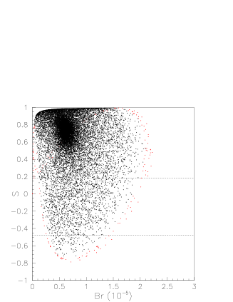
(a)                                             (b)

Figure 4: The correlation between $S_{\phi K_{S}}$ and Br($B\to\phi K_{S}$) for $A_{0}=-1000$GeV. The black (red) dots are allowed by all relevant experimental bounds including (without including) Br($b\rightarrow sg$). (a) is for the SUSY contributions with only gluino propagated in the loop, (b) is for the all contributions included. Current $1\sigma$ bounds are shown by the dashed lines.

We find from Fig. 4 that in both the cases (a) and (b) there are regions of parameters where $S_{\phi K_{S}}$ falls in $1\sigma$ experimental bounds and Br is smaller than $1.6\times 10^{-5}$. In the case of all contributions included the region is larger than that in the case with the contributions from only gluino-squark in the loop included if the constraint from $b\to sg$ is not imposed. There exist two regions of the parameter space as given in Fig. 4 (b) for the all contributions. The dense black region corresponds to the heavy SUSY spectrum region with $m_{0},M_{1/2}$ as large as $600\sim 800$GeV, while the scattered belt region denotes $M_{1/2}$ as small as $100\sim 200$GeV and $m_{0}$ in the region $500\sim 800$GeV where sleptons are as heavy as $500\sim 800$GeV and Br($\tau\to\mu\gamma$) constrains $\delta^{dRR}_{23}$ to be order of $0.1$. That Br($b\rightarrow sg$) serves as a strong constraint on the parameter space is shown in Fig. 4, in particular, the Fig. 4 (b) with all the contributions included. In the scattered belt region of the Fig. 4 (b), with $M_{1/2}$ as small as $100\sim 200$GeV, the destructive chargino contribution to $C_{7\gamma}$ drives $C_{7\gamma}$ smaller than $C^{\rm SM}_{7\gamma}$, which calls for larger $C^{\prime}_{7\gamma}$ of gluino contributions to enhance Br($b\rightarrow s\gamma)\propto|C_{7\gamma}|^{2}+|C^{\prime}_{7\gamma}|^{2}$ above the experimental lower bound. However large $C^{\prime}_{7\gamma}$ results in large $C^{\prime}_{8g}$, which raises Br($b\rightarrow sg$) beyond the experimental upper bound. Therefore, the most of the region without the $b\rightarrow sg$ constraint is excluded when the $b\rightarrow sg$ constraint is imposed. In the case of $A_{0}=0$, Fig. 3 (b) corresponds to only the heavy SUSY spectrum region because the light mass spectrum region, which corresponds to $100GeV\leq m_{0},M_{1/2}\geq 400GeV$ roughly, is excluded by Br($B\to X_{s}\gamma$) and the experimental lower bound of $m_{h^{0}}$ and has no results with $S_{\phi K_{S}}$ near $0$, while Fig. 3 (a), which corresponds to the region of the parameter space with $M_{1/2}$ as small as $100\sim 200$GeV and $m_{0}$ in the region $500\sim 800$GeV, has some results with $S_{\phi K_{S}}$ near $0$, because Br($b\rightarrow s\gamma$) constraints can be satisfied easily in the latter case. Comparing Fig. 4 with Fig. 3, the conclusion is that the SUSY effects on $S_{\phi K_{S}}$ for a negative large $A_{0}$ (say, $|A_{0}|\raise 1.29167pt\hbox{$\;>$\kern-7.5pt\raise-4.73611pt\hbox{$\sim\;$}}m_{0},M_{1/2}$) are larger than those for $A_{0}=0$. The reason is as follows. One needs to have a large $\mu$ in order to have a large RL mixing between down squarks, i.e., a large $\delta^{dRL}_{33}$, and consequently a large induced $\delta^{dRL}_{23}$. Due to the RGE running, a negative large $A_{0}$ can drive $\mu$ at the low energy large, whereas $A_{0}=0$ or a small $A_{0}$ fails. And at the same time, a large $\mu$ can make the chargino contributions significant, which make the real part of $C_{8g}+C_{8g}^{\prime}$ smaller than that in the small $A_{0}$ case.

We vary $\tan\beta$ and find similar results for $\tan\beta=10,30$. The numerical results are obtained for $100GeV\leq m_{0},\;M_{1/2}\leq 800GeV$. For fixed $m_{\tilde{g}}$, the Wilson coefficient $C_{8g}^{(\prime)}$ is not sensitive to the variation of the mass of squark in the range about from $100$GeV to $1500$GeV. Therefore, the numerical results are not sensitive to $m_{0}$ for fixed $M_{1/2}$ and would have a sizable change when $M_{1/2}$ decreases.

VI Conclusions and Discussions

In summary we have calculated the mass spectrum and mixing of sparticles in the SUSY SO(10) GUT. We have calculated the chargino contributions to Wilson coefficients at LO using the MIA with double insertions in SUSY models. Using the Wilson coefficients and hadronic matrix elements previously obtained, we have calculated the time-dependent CP asymmetries $S_{\phi k}$ and branching ratios for the decay $B\rightarrow\phi K_{S}$. It is shown that in the reasonable region of parameters where the constraints from $\tau\to\mu\gamma$, $B_{s}-\bar{B}_{s}$ mixing , $\Gamma(b\to s\gamma)$, $\Gamma(b\to sg)$, $\Gamma(b\to s\mu^{+}\mu^{-})$, and $B\to\mu^{+}\mu^{-}$ are satisfied, the branching ratio of the decay for $B\rightarrow\phi K_{S}$ can be smaller than $1.6\times 10^{-5}$, and $S_{\phi K_{S}}$ can be negative. In some regions of parameters $S_{\phi K_{S}}$ can be as low as $-0.6$.

It is necessary to make a theoretical prediction in SM as precision as we can in order to give a firm ground for finding new physics. For the purpose, we calculate the twist-3 and weak annihilation contributions in SM using the method in Ref. ch by which there is no any phenomenological parameter introduced. The numerical results show that the annihilation contributions to Br are negligible, the twist-3 contributions to Br are also very small, smaller than one percent, and both the annihilation and twist-3 contributions to the time-dependent CP asymmetry are negligible. The conclusion remains in SUSY models and consequently we neglect the annihilation contributions in numerical calculations.

In conclusion, we have shown that the recent experimental measurements on the time-dependent CP asymmetry in $B\to\phi K_{S}$, which can not be explained in SM, can be explained in the SUSY SO(10) grand unification theories where there are flavor non-diagonal right-handed down squark mass matrix elements of second and third generations whose size satisfies all relevant constraints from known experiments ($\tau\to\mu\gamma$, $B\to X_{S}\gamma,B_{s}\to\mu^{+}\mu^{-},B\to X_{s}\mu^{+}\mu^{-},B\to X_{s}g,\Delta M_{s}$, etc.). Therefore, if the present experimental results remain in the future, it will signal the significant breakdown of the standard model and that the SUSY SO(10) GUT is a possible candidate of new physics.

References

Appendix A   Loop functions

In this Appendix, we present the one-loop function of Wilson coefficients in this work.

$$F_{2,12,4,34,6,b0}(x) = x\frac{\partial f_{2,12,4,34,6,b0}(x)}{\partial x}$$

$$F^{\prime}_{2,12,4,34,6,b0}(x) = \frac{x^{2}}{2}\frac{\partial^{2}f_{2,12,4,34,6,b0}(x)}{\partial x^{2}}$$ (62)

with

$$f_{12}(x)=9f_{1}(x)+f_{2}(x),\hskip 28.45274ptf_{34}(x)=9f_{3}(x)+f_{4}(x)/2$$

where $f_{1,2,3,4,6,b0}$ are given in Ref. hw .

References

• (1) Y. Fukuda et al. [Super-Kamiokande Collaboration], Phys. Rev. Lett. 81(1998)1562.
• (2) Q.R. Ahmad et al. [SNO Collaboration], Phys. Rev. Lett. 89(2002)011301; Phys. Rev. Lett. 89(2002)011302.
• (3) K. Eguchi et al. [KamLAND Collaboration], Phys. Rev. Lett. 90(2003)021802.
• (4) M. Apollonio et al.[CHOOZ Collaboration], Phys.Lett.B466(1999)415.
• (5) S. Weinberg, Trans.N.Y.Acad.Sci.38(1977)185; F. Wilczek and A. Zee, Phys. Lett. B70(1977)418; H. Fritzsch, Phys. Lett. B70(1977)436.
• (6) C. D. Froggatt and H. B. Nielsen, Nucl. Phys. B147 (1979) 277.
• (7) K.S. Babu and S.M. Barr, Phys. Lett. B381 (1996) 202; C.H. Albright, K.S. Babu, and S.M. Barr, Phys. Rev. Lett. 81 (1998) 1167; J. Sato and T. Yanagida, Phys. Lett. B430 (1998) 127; N. Irges, S. Lavignac, and P. Ramond, Phys. Rev. D 58 (1998) 035003.
• (8) W. Buchmuller, D.  Delepine and F.  Vissani, Phys. Lett. B459 171 (1999); W. Buchmuller, D. Delepine and L. T. Handoko, Nucl. Phys. B576 445 (2000); J. Ellis, M. E. Gomez, G. K. Leontaris, S. Lola and D. V. Nanopoulos, Eur. Phys. J. C14 319 (2000); J. Hisano and K. Tobe, Phys. Lett. B510 197 (2001); J. A. Casas and A. Ibarra, arXiv:hep-ph/0103065; D. F. Carvalho, J. Ellis, M. E. Gomez and S. Lola, arXiv:hep-ph/0103256; T. Blazek and S. F. King, arXiv:hep-ph/0105005; J. Sato, K. Tobe and T. Yanagida, Phys. Lett. B498 189 (2001); J. Sato and K. Tobe, Phys. Rev. D63 116010 (2001); S. Lavignac, I. Masina and C. A. Savoy, arXiv:hep-ph/0106245; T. Moroi, JHEP. 0003 019 (2000), [arXiv:hep-ph/0002208]; N. Akama, Y. Kiyo, S. Komine and T. Moroi, Phys. Rev. D64 095012 (2001) [arXiv:hep-ph/0104263]; T. Moroi, Phys. Lett. B493, 366 (2000) [arXiv: hep-ph/0007328].
• (9) J. Hisano, T. Moroi, K. Tobe and M. Yamaguchi, Phys. Rev. D53(1996)2442(hep-ph/9510309); J. Hisano and D. Nomura, Phys. Rev. D59(1999)116005(hep-ph/9810479).
• (10) X-J. Bi, Y-B. Dai and X-Y Qi, Phys. Rev.D63 096008 (2001); X-J. Bi and Y-B. Dai, Phys. Rev.D66 076006 (2002).
• (11) D. Chang, A. Masiero and H. Murayama, Phys. Rev. D67 (2003) 075013.
• (12) A. Masiero, S. K. Vempati and O. Vives, Nucl. Phys. B649(2003)189(hep-ph/0209303).
• (13) B. Bajc, G. Senjanovi$\acute{c}$ and F. Vissani, hep-ph/0210207; H.S. Goh, R.N. Mohapatra and S.-P. Ng, hep-ph/0303055.
• (14) J. Hisano and Y. Shimizu, hep-ph/0303071.
• (15) C.-S. Huang, T. Li, W. Liao, Nucl. Phys. B673(2003) 331.
• (16) B. Aubert et al, BABAR Collaboration, Phys. Rev. Lett. 89 (2002) 201802; K. Abe et al, Belle Collaboration, arXiv:hep-ex/0308036.
• (17) Aubert et al. (BABAR Collaboration), hep-ex/0207070; T. Augshev, talk given at ICHEP 2002 (Belle Collaboration), BELLE-CONF-0232; K. Abe et al., BELLE-CONF-0201 hep-ex/0207098.
• (18) The Belle Collaboration, K. Abe et al, hep-ex/0308035(BELLE-CONF-0344); the talk given by T. Browder at LP2003,
http://conferences.fnal.gov/lp2003/program/S5/browder_s05_ungarbled.pdf.
• (19) M. B. Causse, hep-ph/0207070; G. Hiller, Phys. Rev. D66 (2002) 071502;A. Datta, Phys. Rev. D66(2002) 071702; M. Raidal, Phys. Rev. Lett. 89(2002) 231803; K. Agashe and C.D. Carone, hep-ph/0304229; B. Dutta, C.S. Kim, S. Oh, Phys. Rev. Lett. 90 (2003) 011801; J.-P. Lee, K.Y. Lee, hep-ph/0209290; Y.-L. Wu, Y.-F. Zhou, hep-ph/0403252.
• (20) C.-S. Huang and S.-H. Zhu, Phys. Rev. D68 (2003) 114020[arXiv:hep-ph/0307354].
• (21) M. Ciuchini, L. Silvestrini, Phys. Rev. Lett. 89(2002) 231802; L. Silvestrini, hep-ph/0210031(talk contributed at ICHEP02); S. Khalil, E. Kou, Phys. Rev. D67 (2003) 055009; R. Harnik, D.T. Larson, H. Murayama, A. Pierce, hep-ph/0212180; A. Kundu and T. Mitra, hep-ph/0302123; S. Khalil, E. Kou, Phys. Rev. Lett. 91 (2003) 241602;R. Arnowitt, B. Dutta and B. Hu, Phys. Rev. D68 (2003) 075008; J. Hisano, Y. Shimizu, hep-ph/0308255; S. Baek, Phys. Rev. D67 (2003) 096004;D. Chakraverty, E. Gabrielli, K. Huitu, and S. Khalil, Phys. Rev. D68 (2003) 095004.C. Dariescu, M. A. Dariescu, N.G. Deshpande and D. K. Ghosh, hep-ph/0308305; Y. Wang, hep-ph/0309290; V. Barger, C.-W. Chiang, P. Langacker, H.-S. Lee, hep-ph/0310073; S. Mishima, A. I. Sanda, hep-ph/0311068; N. G. Deshpande, D. K. Ghosh, hep-ph/0311332; B. Dutta, C. S. Kim, S. Oh, G. Zhu, hep-ph/0312389; C.H. Chen, C.Q. Geng, hep-ph/0403188.
• (22) G.L. Kane et al., hep-ph/0212092, Phys. Rev. Lett. 90 (2003) 141803.
• (23) A. Stocchi, Nucl. Phys. Proc. Suppl. 117(2003) 145 [arXiv:hep-ph/0211245].
• (24) J.-F. Cheng, C.-S. Huang and X.-H. Wu, Phys. Lett. B 585 (2004) 287 [arXiv:hep-ph/0306086].
• (25) R. Harnik, D.T. Larson, H. Murayama, A. Pierce, hep-ph/0212180.
• (26) M. Ciuchini et al., Phys. Rev. Lett. 92 (2004) 071801.
• (27) K.Abe et. al., Belle collaboration, Phys. Rev. Lett. 92 (2004) 171802 [hep-ex/0310029].
• (28) R. Harnik et al., hep-ph/0212180.
• (29) C.-S. Huang and X.-H. Wu, Nucl. Phys. B657(2003) 304.
• (30) L. J. Hall, V. A. Kostelecky, S. Raby, Nucl. Phys. B267 (1986) 415.
• (31) For a review, see: F. Gabbiani, E. Gabrielli, A. Masiero, L. Silvestrini, Nucl. Phys. B477 (1996) 321.
• (32) H.-n. Li and H. Yu, Phys. Rev. Lett. 74 (1995) 4388; H.-n. Li and T. Yeh, Phys. Rev. D56 (1997) 1615.
• (33) Y. Y. Keum, H.-n. Li and A. I. Sanda, Phys. Lett. B504 (2001) 6; Phys. Rev. D63 (2001) 054008.
• (34) M. Beneke et al., Phys. Rev. Lett. 83(1999) 1914; Nucl. Phys. B591(2000) 313.
• (35) M. Beneke et al., Nucl. Phys. B606(2001) 245.
• (36) Y. Nir, Nucl. Phys. Proc. Suppl. 117 (2003) 111.
• (37) S. Dimopoulos and L.J. Hall, Phys. Lett. B344, 185 (1995).
• (38) M. Gell-Mann, P. Rammond and R. Slansky, in Supergravity, eds. D. Freedman et al. (North-Holland, Amsterdam, 1980); T. Yanagida, in proc. KEK workshop, 1979 (unpublished); R.N. Mohapatra and G. Senjanović, Phys. Rev. Lett. 44, 912 (1980); S. L. Glashow, Cargese lectures, (1979).
• (39) W. Buchmueller and D. Wyler, Phys. Lett. B521, 291 (2001).
• (40) G. Buchalla, A. J. Buras and M. E. Lautenbacher, Rev. Mod. Phys.  68, 1125 (1996) [arXiv:hep-ph/9512380].
• (41) L. Everett, G. L. Kane, S. Rigolin, L. -T. Wang, and T. T. Wang, JHEP 0201 (2002) 022.
• (42) E. Lunghi, A. Masiero, I. Scimemi, and L. Silvestrini, Nucl. Phys. B568 (2000) 120.
• (43) J.A. Bagger, K.T. Matchev and R.J. Zhang, Phys. Lett. B412(1997) 77; M. Ciuchini et al., Nucl. Phys. B523(1998) 501; C.-S. Huang and Q.-S. Yan, ”The frontiers of physics at millennium” (Beijing 1999), Editor Y.-L. Wu, p.129 [hep-ph/9906493]; A.J. Buras, M. Misiak and J. Urban, Nucl.Phys. B586 (2000) 397.
• (44) F. Borzumati, C. Greub, T. Hurth and D. Wyler, Phys. Rev. D62(2000) 075005 .
• (45) G. Hiller, F. Kr$\ddot{u}$ger, hep-ph/0310219.
• (46) J.-F. Cheng, C.-S. Huang and X.-H. Wu, hep-ph/0404055.
• (47) X.-G. He, J.P. Ma and C.-Y. Wu, Phys. Rev. D63 (2001) 094004; H.-Y. Cheng and K.C. Yang, Phys. Rev. D64(2001) 074004.
• (48) Y. Y. Keum, H. n. Li and A. I. Sanda, Phys. Lett. B 504, 6 (2001) [arXiv:hep-ph/0004004].
• (49) B.V. Geshkenbein and M.V. Terentev, Phys. Lett. 117, 243 (1982).
• (50) T. Feldmann, P. Kroll and B. Stech, Phys. Rev. D 58, 114006 (1998) [hep-ph/9802409];
T. Feldmann, Int. J. Mod. Phys. A 15, 159 (2000) [hep-ph/9907491].
• (51) R. Kaiser and H. Leutwyler, Proceedings of Workshop on Nonperturbative Methods in Quantum Field Theory, Adelaide, 1998 [hep-ph/9806336];
R. Kaiser and H. Leutwyler, Eur. Phys. J. C 17 (2000) 623 [hep-ph/0007101].
• (52) M. Ciuchini et al, J. High Energy Phys. 07(2001), 13
• (53) Hai-Yang Cheng, Yong-Yeon Keum and Kwei-Chou Yang, Phys.Rev.D65 (2002) 094023.
• (54) D. Acosta et al. (CDF Collaboration), hep-ex/0403032.
• (55) K. Hagiwara et al., Phys. Rev. D66, 010001 (2002).
• (56) J.L. Lopez, D.V. Nanopoulos, X. Wang and A. Zichichi, Phys. Rev. D51, 147 (1995).
• (57) Y.-B. Dai, C.-S. Huang and H.-W. Huang, Phys. Lett. B390(1997) 257; C.-S. Huang and Q.-S. Yan, Phys. Lett. B442(1998) 209; C.-S. Huang, W. Liao, and Q.-S. Yan, Phys. Rev. D59(1999) 011701.
• (58) N. Chamoun, C.-S. Huang, C. Liu, X.-H. Wu, Nucl. Phys. B624 (2002) 81.
• (59) A. Kagan, hep-ph/9806266; T.E. Coan et al. (CLEO Collaboration), Phys. Rev. Lett. 80, 1150 (1998).
• (60) R. Harnik, D. T. Larson, H. Murayama, A. Pierce, arXiv:hep-ph/0212180.
• (61) J.-F. Cheng and C.-S. Huang, Phys. Lett. B554(2003) 155 . In the paper the constraint from $B\to\mu^{+}\mu^{-}$ is not imposed.
• (62) D. Acosta et al. (CDF Collaboration), hep-ex/0403032.
• (63) T.Ibrahim and P.Nath, Phys.Rev. D57,478(1998); (E) ibid, D58, 019901(1998); Phys. Rev. D58,111301(1998); M.Brhlik,G.J.Good,and G.L.Kane, Phys. Rev. D59,11504(1999); C.-S. Huang and Liao Wei, Phys. Rev. D61 (2000) 116002; ibid. D62 (2000) 016008.