Higgs Boson Resummation via Bottom-Quark Fusion

Abstract

The region of small transverse momentum in $q\bar{q}-$ and $gg-$initiated processes must be studied in the framework of resummation to account for the large, logarithmically-enhanced contributions to physical observables. In this letter, we study resummed differential cross-sections for Higgs production via bottom-quark fusion. We find that the differential distribution peaks at approximately $15$ GeV, a number of great experimental importance to measuring this production channel.

Resummation of total and differential cross-section for the inclusive production of a Higgs boson has concentrated on the gluon-gluon initial stateCatani:ne ; Kauffman:1991jt ; Yuan:1991we ; Kauffman:cx ; Catani:1996yz ; Kramer:1996iq ; Balazs:2000wv ; deFlorian:2000pr ; deFlorian:2001zd ; Glosser:2002gm ; Berger:2002ut ; Berger:2003pd ; Bozzi:2003jy ; Field:2004tt . In the Standard Model (sm), the gluon-gluon initial state gives the largest contribution to the total and differential cross-sections, but this is not always the case in extensions of the sm. In the Minimal Supersymmetric Standard Model (mssm) the bottom-quark fusion initial state can be greatly enhanced, perhaps leading to the observation of a supersymmetric signal in nature, if the location of the peak of the differential distribution in known.

The mssm contains two Higgs doublets, one giving mass to up-type quarks and the other to down-type quarks. The associated vacuum expectation values (vevs) are labeled $v_{u}$ and $v_{d}$ respectively, and fix the free mssm parameter $\tan\beta\equiv v_{u}/v_{d}$. In the mssm, there are five physical Higgs boson mass eigenstates. In this letter, we are interested in the neutral Higgs bosons $\{h^{0},H^{0},A^{0}\}$ which we will call $\Phi$ generically.

In contrast to the sm, the bottom-quark Yukawa couplings in the mssm can be enhanced with respect to the top-quark Yukawa coupling. In the sm, the ratio of the $t\bar{t}\Phi$ and $b\bar{b}\Phi$ couplings is given at tree-level by $\lambda^{\textsc{sm}}_{t}/\lambda^{\textsc{sm}}_{b}=m_{t}/m_{b}\approx 35$. In the mssm, the coupling depends on the value of $\tan\beta$. At leading order,

$$\frac{\lambda^{\textsc{mssm}}_{t}}{\lambda^{\textsc{mssm}}_{b}}=f_{\Phi}\,\frac{1}{\tan\beta}\cdot\frac{m_{t}}{m_{b}}\,,$$ (1)

with

$$f_{\Phi}=\left\{\begin{array}[]{ll}-\cot\alpha\,,&\qquad\Phi=h^{0}\\ \phantom{-}\tan\alpha\,,&\qquad\Phi=H^{0}\\ \phantom{-}\cot\beta\,,&\qquad\Phi=A^{0}\end{array}\right.$$ (2)

where $\alpha$ is the mixing angle between the weak and the mass eigenstates of the neutral scalars. Given the mass of the pseudoscalar $M_{A^{0}}$ and $\tan\beta$, the angle $\alpha$ can be determined given reasonable assumptions for the masses of the other supersymmetric particles in the spectrum.

The form of $f_{\Phi}$ shows us that the production of the pseudoscalar due to bottom-quark fusion is enhanced by a factor of $\tan^{2}\!\beta$, which is a free parameter in the theory.

I The Bottom-Quark

It is also important to define what is meant by a bottom-quark distributionOlness:1987ep ; Barnett:1987jw ; Olness:1997yc . In our analysis, we employed the CTEQ6.1M bottom-quark parton distributionPumplin:2002vw with $\alpha_{\textrm{s}}(M_{Z})=0.118$ and set the mass of the Higgs boson of interest $M_{\Phi}=120$ GeV. We compared the bottom-quark distribution function in the PDF set and the numeric solution to the Dokshitzer-Gribov-Lipatov-Altarelli-Parisi (dglap) equations for a single quark splitting. A bottom-quark distribution for a gluon splitting into a $b\bar{b}$ pair can be written in the dglap formalism as

$$\tilde{b}(x,\mu)=\frac{\alpha_{\textrm{s}}(\mu)}{2\pi}\ln\biggl{(}\frac{\mu^{2}}{m_{b}^{2}}\biggr{)}\int_{x}^{1}\frac{dy}{y}P_{q\leftarrow g}\biggl{(}\frac{x}{y}\biggr{)}g(y,\mu),$$ (3)

where $g$ is the gluon distribution, and the dglap splitting function is

$$P_{q\leftarrow g}(z)=\frac{1}{2}[z^{2}+(1-z)^{2}].$$ (4)

The bottom-quark distribution is encoded into the CTEQ PDF set in this mannerfred , but takes into account multiple quark splitting functions. When evaluated with the dglap formalism, we found the differential cross-section increased by approximately $10$% near its peak. However, we used the native bottom-quark distributions for speed and to understand their built-in uncertainties.

PreviouslyField:2004tt , we calculated in detail the resummation coefficients for a differential cross-section for the scalar and pseudoscalar Higgs boson from the gluon-gluon initial state. In this letter, we will calculate the resummation coefficients needed for the resummation of the $b\bar{b}$ initial state for the scalar and pseudoscalar Higgs bosons in the same manner as the gluon-gluon channel in Ref. Field:2004tt . We will leave the bottom-quark–Higgs coupling set equal to the sm value so that the reader can scale the results to whatever coupling value is of interest.

II Resummation

The resummation formalism needs the lowest order total cross-section as a normalization factor (see Field:2004tt for details), $b\bar{b}\rightarrow\Phi$ in this case. Following Ref. Harlander:2003ai , we will ignore the bottom-quark mass except in the Yukawa coupling with the Higgs boson. Although the pseudoscalar Higgs couples to quarks with a $\gamma_{5}$, there are no differences in the matrix elements (modulo the mssm coupling factor) when the bottom-quark mass is neglected.

It is important to use the $\overline{\textrm{MS}}$ running mass for the bottom-quark in our calculation as the difference from the pole mass at the scales involved is considerableDicus:1998hs ; Campbell:2002zm . In the sm, the bottom-quark Yukawa coupling is $\lambda_{b}^{\textsc{sm}}=\sqrt{2}\overline{m}_{b}/v$, where $v$ is the sm vev and is approximately equal to $246$ GeV and $\overline{m}_{b}$ is the $\overline{\textrm{MS}}$ running mass. We have set the bottom-quark mass $\overline{m}_{b}(\overline{m}_{b})=4.62$ GeV in our calculations. The NLO running of the bottom-quark mass corresponds to $\overline{m}_{b}(M_{\Phi})=3.23$ GeV. The coupling in the mssm can be written

$$\begin{split}\lambda_{b}^{\textsc{mssm}}&=\left\{\begin{array}[]{ll}\displaystyle-\sqrt{2}\,\frac{\overline{m}_{b}}{v}\frac{\sin\alpha}{\cos\beta}\,,&\qquad\Phi=h^{0}\\[15.0pt] \displaystyle\phantom{-}\sqrt{2}\,\frac{\overline{m}_{b}}{v}\frac{\cos\alpha}{\cos\beta}\,,&\qquad\Phi=H^{0}\\[15.0pt] \displaystyle\phantom{-}\sqrt{2}\,\frac{\overline{m}_{b}}{v}\tan\beta\,,&\qquad\Phi=A^{0}.\end{array}\right.\end{split}$$ (5)

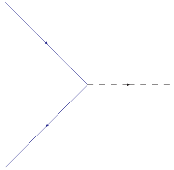
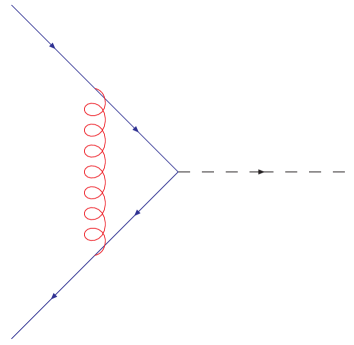
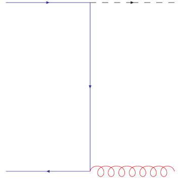
(a)	(b)	(c)

Figure 1: Diagrams needed for the $b\bar{b}$ initial state resummed differential cross-section. Figure 1a is the lowest order production channel and couples differently for different Higgs bosons. Figure 1b is the virtual correction to the lowest order process. Figure 1c is the lowest order graph contributing to the differential cross-section. The crossed graph is not shown.

The spin- and color-averaged total partonic cross-section (see Fig. 1a) for the leading order subprocess, $b\bar{b}\rightarrow\Phi$, can be easily written

$$\hat{\sigma}_{0}^{\textsc{sm}}=\frac{6\pi}{4N_{c}^{2}}\frac{\overline{m}_{b}^{2}}{v^{2}}\frac{1}{M_{\Phi}^{2}}\delta(1-z),$$ (6)

where $z=M_{\Phi}^{2}/\hat{s}$ and the number of colors $N_{c}=3$. We also need the LO differential cross-section (Fig. 1c) for the next-to-leading log (NLL) resummation coefficients for the differential cross-section. If we remove the $\delta(1-z)$ factor from our prefactor $\hat{\sigma}_{0}$, then we can write the spin- and color-averaged differential cross-section for $b(p_{1})\bar{b}(p_{2})\rightarrow g(-p_{3})\Phi(-p_{5})$ as

$$\frac{d\hat{\sigma}}{d\hat{t}} =\hat{\sigma}_{0}\biggl{(}\frac{\alpha_{\textrm{s}}}{\pi}\biggr{)}\frac{{C_{F}}}{2}\biggl{(}\frac{M_{\Phi}^{4}+\hat{s}^{2}}{\hat{s}\hat{t}\hat{u}}\biggr{)}$$

$$=\hat{\sigma}_{0}\biggl{(}\frac{\alpha_{\textrm{s}}}{\pi}\biggr{)}\frac{{C_{F}}}{2}\frac{1}{p_{t}^{2}}\biggl{[}1+z^{2}\biggr{]}.$$ (7)

where ${C_{F}}=(N_{c}^{2}-1)/2N_{c}$, and the kinematic variables are defined as $\hat{s}=(p_{1}+p_{2})^{2}$, $\hat{t}=(p_{1}+p_{5})^{2}$, $\hat{u}=(p_{2}+p_{5})^{2}$, and $M_{\Phi}^{2}=p_{5}^{2}$. In our second line, we have written the differential cross-section in terms of $\hat{u}\hat{t}=p_{t}^{2}\hat{s}$ for the $2\rightarrow 2$ process.

To find the resummation coefficients for a differential cross-sectionsKauffman:1991jt ; Kauffman:cx ; deFlorian:2001zd ; Field:2004tt we integrate the differential cross-section around $p_{t}=0$

$$\Delta\hat{\sigma}=\int_{0}^{q_{t}^{2}}dp_{t}^{2}\frac{d\hat{\sigma}}{dp_{t}^{2}}$$ (8)

and label this result ‘real’ as it is similar to the real corrections to the LO total cross-section. Working in $N=4-2\epsilon$ dimensions, we find

$$\Delta\hat{\sigma}^{\textrm{real}}=\hat{\sigma}_{0}z\frac{\alpha_{\textrm{s}}}{\pi}\biggl{[} \frac{{C_{F}}}{\epsilon^{2}}+\frac{3}{2}\frac{{C_{F}}}{\epsilon}-\frac{{C_{F}}}{2}\ln^{2}\biggl{(}\frac{M_{\Phi}^{2}}{q_{t}^{2}}\biggr{)}$$

$$+ \frac{3}{2}{C_{F}}\ln\biggl{(}\frac{M_{\Phi}^{2}}{q_{t}^{2}}\biggr{)}+{C_{F}}-{C_{F}}{\zeta_{2}}\biggr{]}.$$ (9)

To regularize this result, we need to add the virtual corrections that are shown in Fig. 1b. These corrections are very similar to Drell-Yan correctionsAltarelli:1979ub . The virtual corrections can be written as

$$\Delta\hat{\sigma}_{\textrm{virt}}=\hat{\sigma}_{0}\biggl{(}\frac{\alpha_{\textrm{s}}}{\pi}\biggr{)}\biggl{[}-\frac{{C_{F}}}{\epsilon^{2}}-\frac{3}{2}\frac{{C_{F}}}{\epsilon}-{C_{F}}+2{C_{F}}{\zeta_{2}}\biggr{]}.$$ (10)

In the Drell-Yan case, the $-{C_{F}}$ factor would be $-4{C_{F}}$. When the two results are added together the resummation coefficients are easily read off from the expression. The total expression is

$$\Delta\hat{\sigma}=\hat{\sigma}_{0}z\biggl{[}1 +\frac{\alpha_{\textrm{s}}}{\pi}\biggl{(}-\frac{{C_{F}}}{2}\ln^{2}\biggl{(}\frac{M_{\Phi}^{2}}{q_{t}^{2}}\biggr{)}$$

$$+\frac{3}{2}{C_{F}}\ln\biggl{(}\frac{M_{\Phi}^{2}}{q_{t}^{2}}\biggr{)}+{C_{F}}{\zeta_{2}}\biggr{)}\biggr{]}.$$ (11)

Keeping with the notation of Ref. Field:2004tt , we write these coefficients with an overbar as follows

$$\bar{A}^{(1)}_{b}={{C_{F}}},\quad\bar{B}^{(1)}_{b}=-\frac{3}{2}{{C_{F}}},\quad\bar{C}^{(1)}_{b\bar{b}}=\frac{1}{2}{{C_{F}}}{\zeta_{2}}.$$ (12)

It is important to note that in contrast to $W^{\pm}/Z^{0}$ production and Drell-Yan processesAltarelli:1979ub ; Arnold:1990yk , the $\bar{C}^{(1)}$ coefficient is positive.

Finally, let us turn to determining the $C^{(1)}$ and $C^{(2)}$ coefficients for the total cross-section resummation, although total cross-sections will not be presented in this letter. Using the results of Ref. Harlander:2003ai , we take the Mellin moments of the corrections in the limit $N\rightarrow\infty$ ($z\rightarrow 1$ in $z$-space). The NLO corrections are easy to color decompose due to the presence of only one color factorField:2004tt . Leaving the terms that were originally proportional to the $\delta(1-z)$ factor inside curly brackets, we find

$$\Delta_{b\bar{b}}^{(1)}=\biggl{[} 2{{C_{F}}}\biggr{]}{\ln^{2}(N)}+\biggl{[}2{{C_{F}}}{\,\ln\!\frac{M^{2}_{\Phi}}{\mu_{f}^{2}}}\biggr{]}{\ln(N)}$$

$$+\biggl{\{} 2{{C_{F}}}{\zeta_{2}}-{{C_{F}}}+2{\,\ln\!\frac{\mu_{r}^{2}}{\mu_{f}^{2}}}\biggr{\}}+2{{C_{F}}}{\zeta_{2}}$$ (13)

where we have given both the renormalization scale $\mu_{r}$ and the factorization scale $\mu_{f}$ dependence in the results.

In contrast to NLO, the NNLO corrections contain a mix of color factors (both ${C_{A}}$ and ${C_{F}}$ appear). Although it is easy to see that the factor proportional to $\ln^{4}(N)$ should clearly be $2{C^{2}_{F}}$, no unique color decomposition from the results provided in Ref. Harlander:2003ai can be determined for all the terms in the expression. However, the numeric result can be written

$$\Delta_{b\bar{b}}^{(2)} =\biggl{[}\frac{32}{9}\biggr{]}\!{\ln^{4}(N)}+\biggl{[}\frac{44}{9}-\frac{8}{27}{n_{\!f}}+\frac{64}{9}{\,\ln\!\frac{M^{2}_{\Phi}}{\mu_{f}^{2}}}\biggr{]}\!{\ln^{3}(N)}$$

$$+\biggl{[}\frac{34}{3}+\frac{92}{9}{\zeta_{2}}-\frac{20}{27}{n_{\!f}}+\biggl{(}\frac{38}{3}-\frac{4}{9}{n_{\!f}}\biggr{)}{\,\ln\!\frac{M^{2}_{\Phi}}{\mu_{r}^{2}}}$$

$$-\frac{16}{3}{\,\ln\!\frac{M^{2}_{\Phi}}{\mu_{f}^{2}}}+\frac{32}{9}{\,\ln^{2}\!\frac{M^{2}_{\Phi}}{\mu_{f}^{2}}}\biggr{]}\!{\ln^{2}(N)}+\biggl{[}\frac{404}{27}-14{\zeta_{3}}$$

$$-\frac{56}{81}{n_{\!f}}+\biggl{(}\frac{34}{3}+\frac{92}{9}{\zeta_{2}}-\frac{20}{27}{n_{\!f}}\biggr{)}{\,\ln\!\frac{M^{2}_{\Phi}}{\mu_{f}^{2}}}-\biggl{(}9-\frac{2}{9}{n_{\!f}}\biggr{)}$$

$$\times{\,\ln^{2}\!\frac{M^{2}_{\Phi}}{\mu_{f}^{2}}}+\biggl{(}\frac{38}{3}-\frac{4}{9}{n_{\!f}}\biggr{)}{\,\ln\!\frac{M^{2}_{\Phi}}{\mu_{r}^{2}}}{\,\ln\!\frac{M^{2}_{\Phi}}{\mu_{f}^{2}}}\biggr{]}\!{\ln(N)}+\biggl{\{}\frac{115}{18}$$

$$+\frac{58}{9}{\zeta_{2}}-\frac{26}{3}{\zeta_{3}}-\frac{19}{18}{\zeta_{4}}+\biggl{(}\frac{2}{27}-\frac{10}{27}{\zeta_{2}}+\frac{2}{3}{\zeta_{3}}\biggr{)}{n_{\!f}}$$

$$+\biggl{(}\frac{25}{12}+\frac{38}{3}{\zeta_{2}}\biggr{)}{\,\ln\!\frac{M^{2}_{\Phi}}{\mu_{r}^{2}}}-\biggl{(}\frac{1}{18}+\frac{4}{9}{\zeta_{2}}\biggr{)}{n_{\!f}}{\,\ln\!\frac{M^{2}_{\Phi}}{\mu_{r}^{2}}}$$

$$+\biggl{(}\frac{11}{12}-10{\zeta_{2}}-\frac{122}{9}{\zeta_{3}}\biggr{)}{\,\ln\!\frac{M^{2}_{\Phi}}{\mu_{f}^{2}}}+\biggl{(}\frac{1}{18}+\frac{4}{9}{\zeta_{2}}\biggr{)}{n_{\!f}}{\,\ln\!\frac{M^{2}_{\Phi}}{\mu_{f}^{2}}}$$

$$+\biggl{(}\frac{19}{4}-\frac{1}{6}{n_{\!f}}\biggr{)}{\,\ln^{2}\!\frac{M^{2}_{\Phi}}{\mu_{r}^{2}}}+\biggl{(}\frac{19}{4}-\frac{32}{9}{\zeta_{2}}-\frac{1}{6}{n_{\!f}}\biggr{)}{\,\ln^{2}\!\frac{M^{2}_{\Phi}}{\mu_{f}^{2}}}$$

$$+\biggl{(}\frac{1}{3}{n_{\!f}}-\frac{19}{2}\biggr{)}{\,\ln\!\frac{M^{2}_{\Phi}}{\mu_{r}^{2}}}{\,\ln\!\frac{M^{2}_{\Phi}}{\mu_{f}^{2}}}\biggr{\}}+\frac{34}{3}{\zeta_{2}}+\frac{88}{9}{\zeta_{3}}+\frac{364}{45}{\zeta_{2}^{2}}$$

$$-\biggl{(}\frac{20}{27}{\zeta_{2}}+\frac{16}{27}{\zeta_{3}}\biggr{)}{n_{\!f}}+\biggl{(}\frac{38}{3}{\zeta_{2}}-\frac{4}{9}{\zeta_{2}}{n_{\!f}}\biggr{)}{\,\ln\!\frac{M^{2}_{\Phi}}{\mu_{r}^{2}}}$$

$$-\biggl{(}\frac{16}{3}{\zeta_{2}}-\frac{128}{9}{\zeta_{3}}\biggr{)}{\,\ln\!\frac{M^{2}_{\Phi}}{\mu_{f}^{2}}}+\frac{32}{9}{\zeta_{2}}{\,\ln^{2}\!\frac{M^{2}_{\Phi}}{\mu_{f}^{2}}}$$ (14)

We can also determine the NNLL $A^{(2)}$ and $B^{(2)}$ coefficients. $A^{(2)}$ agrees with a previous calculationBalazs:1998sb . We find

$$A^{(1)}_{b} ={{C_{F}}}$$ (15)

$$A^{(2)}_{b} =\frac{1}{2}{{C_{F}}}\biggl{(}{{C_{A}}}\biggl{(}\frac{67}{18}-{\zeta_{2}}\biggr{)}-\frac{10}{9}{{n_{\!f}}{T_{\!R}}}\biggr{)}$$ (16)

for $A^{(1)}$ and $A^{(2)}$ and

$$B^{(1)}_{b}=-\frac{3}{2}{{C_{F}}}$$ (17)

$$B^{(2)}_{b} ={{C^{2}_{F}}}\biggl{(}\frac{3}{2}{\zeta_{2}}-3{\zeta_{3}}-\frac{3}{16}\biggr{)}$$

$$-{{C_{A}}{C_{F}}}\biggl{(}\frac{11}{18}{\zeta_{2}}-\frac{3}{2}{\zeta_{3}}+\frac{13}{16}\biggr{)}$$

$$-{{n_{\!f}}{C_{F}}{T_{\!R}}}\biggl{(}\frac{1}{4}+\frac{2}{9}{\zeta_{2}}\biggr{)}$$ (18)

for the $B^{(1)}$ and $B^{(2)}$ coefficients. The Mellin moments $\Delta^{(1)}_{b\bar{b}}$ and $\Delta^{(2)}_{b\bar{b}}$ are novel, as is $B^{(2)}_{b}$.

III Results and Conclusions

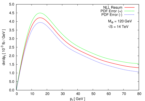
(a)

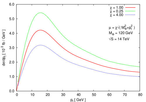
(b)

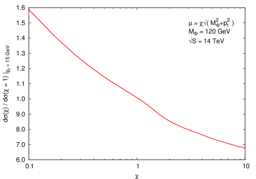
(c)

Figure 2: Figure 2a shows the errors associated with the CTEQ6.1M PDF set. The variation is approximately $8-12$%. Figure 2b show the variation of the renormalization and factorization scale for a factor of $1/4$ and $4$. These scales were chosen because there has been great interest in the scale $\mu=M_{\Phi}/4$. We find this variation to be approximately $20$%. Figure 2c shows the movement of the peak of the differential distribution (at $15$ GeV) for a variation in the scale by a factor of $10$.

The differential resummation coefficients and the position of the peak of the differential cross-section is of great interest to the experimental community involved with Higgs research at the LHC, particularly in the $M_{\Phi}=120$ GeV mass range. Here the Higgs will decay primarily into $b\bar{b}$ pairs that can be tagged. Knowing where the peak of the differential distribution lies, especially if it is below the $p_{t}$ of a typical trigger event, is of utmost importance. This letter will help in the analysis of the $b\bar{b}$ initial state.

The results of our calculations can be found in Figure 2. We have done our analysis for the LHC (a proton-proton collider at $\sqrt{S}=14$ TeV). We find that the differential distribution at the LHC peaks at a transverse momentum of approximately $15$ GeV. We find that the magnitiude of the differential cross-section is an excellent match with previously published resultsDicus:1998hs ; Balazs:1998sb ; Campbell:2002zm . The results for the Tevatron are extremely similar, but are smaller by a factor of $60$ and the peak moves to a transverse momentum of approximately $13$ GeV in the differential distribution.

A detailed study of the uncertainties in the calculation show that the uncertainty due to the PDF set is approximately $8-12$%. At the peak of the distribution, the uncertainty is approximately $10$% due to the PDFs. When the scale is varied by a factor of four, we see a variation in the differential cross-section of approximately $20$%. This would give us a combined uncertainty of $32$%, which is slightly better than the gluon-gluon channelField:2004tt uncertainty in the differential distribution. However, when the scale is only varied by a factor of two (as was the case for the gluon-gluon channel), the total uncertainty drops to $25$%.

We have calculated the resummation coefficients needed for NLL inclusive Higgs production via bottom-quark fusion in the sm and the mssm for the differential cross-section and for the NNLL resummation for the total cross-section. We find a smaller uncertainty in the bottom-quark initial state than the gluon-gluon initial state.

References

• (1) S. Catani and L. Trentadue, Nucl. Phys. B 327, 323 (1989).
• (2) R. P. Kauffman, Phys. Rev. D 44, 1415 (1991).
• (3) C. P. Yuan, Phys. Lett. B 283, 395 (1992).
• (4) R. P. Kauffman, Phys. Rev. D 45, 1512 (1992).
• (5) S. Catani, M. L. Mangano, P. Nason and L. Trentadue, Nucl. Phys. B 478, 273 (1996) [arXiv:hep-ph/9604351].
• (6) M. Kramer, E. Laenen and M. Spira, Nucl. Phys. B 511, 523 (1998)
• (7) C. Balazs and C. P. Yuan, Phys. Lett. B 478, 192 (2000) [arXiv:hep-ph/0001103].
• (8) D. de Florian and M. Grazzini, Phys. Rev. Lett.  85, 4678 (2000) [arXiv:hep-ph/0008152].
• (9) D. de Florian and M. Grazzini, Nucl. Phys. B 616, 247 (2001) [arXiv:hep-ph/0108273].
• (10) C. J. Glosser and C. R. Schmidt, JHEP 0212, 016 (2002) [arXiv:hep-ph/0209248].
• (11) E. L. Berger and J.-w. Qiu, Phys. Rev. D 67, 034026 (2003) [arXiv:hep-ph/0210135].
• (12) E. L. Berger and J.-w. Qiu, Phys. Rev. Lett.  91, 222003 (2003) [arXiv:hep-ph/0304267].
• (13) G. Bozzi, S. Catani, D. de Florian and M. Grazzini, Phys. Lett. B 564, 65 (2003) [arXiv:hep-ph/0302104].
• (14) B. Field, In Press, Phys. Rev. D, [arXiv:hep-ph/0405219].
• (15) F. I. Olness and W. K. Tung, Nucl. Phys. B 308, 813 (1988).
• (16) R. M. Barnett, H. E. Haber and D. E. Soper, Nucl. Phys. B 306, 697 (1988).
• (17) F. I. Olness, R. J. Scalise and W. K. Tung, Phys. Rev. D 59, 014506 (1999) [arXiv:hep-ph/9712494].
• (18) J. Pumplin, D. R. Stump, J. Huston, H. L. Lai, P. Nadolsky and W. K. Tung, JHEP 0207, 012 (2002) [arXiv:hep-ph/0201195].
• (19) F. I. Olness, private communication.
• (20) R. V. Harlander and W. B. Kilgore, Phys. Rev. D 68, 013001 (2003) [arXiv:hep-ph/0304035].
• (21) J. Campbell, R. K. Ellis, F. Maltoni and S. Willenbrock, Phys. Rev. D 67, 095002 (2003) [arXiv:hep-ph/0204093].
• (22) D. Dicus, T. Stelzer, Z. Sullivan and S. Willenbrock, Phys. Rev. D 59, 094016 (1999) [arXiv:hep-ph/9811492].
• (23) G. Altarelli, R. K. Ellis and G. Martinelli, Nucl. Phys. B 157, 461 (1979).
• (24) P. B. Arnold and R. P. Kauffman, Nucl. Phys. B 349, 381 (1991).
• (25) C. Balazs, H. J. He and C. P. Yuan, Phys. Rev. D 60, 114001 (1999) [arXiv:hep-ph/9812263].