CERN-PH-TH/2004-137

hep-ph/0407241

The back-to-back region
in $e^{+}e^{-}$ energy–energy correlation

Daniel de Florian${}^{\,a}$   and   Massimiliano Grazzini${}^{\,b}$

${}^{a}\,$Departamento de Física, FCEYN, Universidad de Buenos Aires, (1428) Pabellón 1 Ciudad Universitaria, Capital Federal, Argentina

${}^{b}\,$Department of Physics, Theory Division, CERN, CH-1211 Geneva 23, Switzerland

Abstract

We consider the back-to-back region in the energy–energy correlation in $e^{+}e^{-}$ collisions. We present the explicit expression of the ${\cal O}(\alpha_{\mathrm{S}}^{2})$ logarithmically enhanced contributions up to next-to-next-to-leading logarithmic accuracy. We study the impact of the results in a detailed comparison with precise LEP and SLC data. We find that, when hadronization effects are taken into account as is customarily done in QCD analysis in $e^{+}e^{-}$ annihilations, the extracted value of $\alpha_{\mathrm{S}}(M_{Z})$ is in good agreement with the current world average.

hep-ph/0407241

July 2004

1 Introduction

Precise data on $e^{+}e^{-}$ annihilation into hadrons have provided detailed experimental tests of QCD and one of the best opportunities to measure the strong coupling constant $\alpha_{\mathrm{S}}$. A particularly well suited observable is the energy–energy correlation (EEC) [1], defined as an energy-weighted correlation for the cross section corresponding to the process $e^{+}e^{-}\rightarrow h_{a}+h_{b}+X$ as

$$\frac{1}{\sigma_{T}}\frac{d\Sigma}{d\cos\chi}=\frac{1}{\sigma_{T}}\sum_{a,b}\int\frac{E_{a}\,E_{b}}{Q^{2}}d\sigma_{e^{+}e^{-}\rightarrow h_{a}h_{b}+X}\,\delta(\cos\chi+\cos\theta_{ab})\,,$$ (1)

where $E_{a}$ and $E_{b}$ are the energies of the particles, $Q$ is the centre-of-mass energy, $\theta_{ab}\equiv\pi-\chi$ is the angle between the two hadrons, and $\sigma_{T}$ is the total cross section for $e^{+}e^{-}\rightarrow{\rm hadrons}$.

The two-hadron cross section $e^{+}e^{-}\rightarrow h_{a}+h_{b}+X$ depends on the fragmentation functions of the partons into the final-state hadrons. However, thanks to the momentum sum rule

$$\sum_{h}\int_{0}^{1}dxxD_{h/q}(x,\mu_{F}^{2})=1\,,$$ (2)

EEC becomes independent of them, and can thus be computed in QCD perturbation theory.

Theoretical calculations [2, 3, 4] for the EEC function have been performed up to next-to-leading order (NLO) accuracy in QCD [5]–[12], allowing a detailed comparison with the available data.

As is well known, fixed-order calculations have a limited kinematical range of applicability. In the back-to-back region, defined by $\theta_{ab}\rightarrow\pi$ ($\chi\rightarrow 0$), the multiple emission of soft and collinear gluons gives rise to large logarithmic contributions of the form $\alpha_{\mathrm{S}}^{n}\log^{2n-1}y$, where $y=\sin^{2}\chi/2$. As $y$ decreases, the logarithms become large and therefore invalidate the use of the fixed-order perturbative expansion.

These logarithmic contributions can be resummed to all orders [13, 14]. The resummation formalism is very close to the one developed for the transverse-momentum distribution of high-mass systems in hadronic collisions . When the transverse momentum $q_{T}^{2}$ of the detected final state is much smaller than its invariant mass $Q^{2}$, large logarithmic contributions $\alpha_{\mathrm{S}}^{n}\log^{2n-1}q_{T}^{2}/Q^{2}$ arise which must be resummed to all orders.

The coefficients that control the resummation at a given order can be computed if an analytical calculation at the same order exists. In the case of hadronic collisions, the complete form of the logarithmically enhanced contributions has been computed [15]. In this paper we present the result of a similar calculation, performed for EEC. Our calculation allows us to fix the still missing coefficients at ${\cal O}(\alpha_{\mathrm{S}}^{2})$ and to extend the resummation for this observable to full next-to-next-to-leading logarithmic (NNLL) accuracy. We also study the numerical impact of our results and present a comparison with LEP and SLC data.

The paper is organized as follows. In Sect. 2 we review the resummation formalism and we discuss the results of our calculation. In Sect. 3 we present numerical results, and we also consider the inclusion of hadronization effects. In particular, we perform a fit to OPAL and SLD data.

2 Soft-gluon resummation

The EEC function can be decomposed as

$$\frac{1}{\sigma_{T}}\frac{d\Sigma}{d\cos\chi}=\frac{1}{\sigma_{T}}\frac{d\Sigma^{\rm(res.)}}{d\cos\chi}+\frac{1}{\sigma_{T}}\frac{d\Sigma^{\rm(fin.)}}{d\cos\chi}\,;$$ (3)

the first term on the right-hand side of Eq. (3) contains all the logarithmically enhanced contributions, $\alpha_{\mathrm{S}}^{n}/y\log^{m}y$ at small $y$ and has to be evaluated by resumming them to all orders. The second is free of such contributions and can be computed by using fixed-order perturbation theory.

The resummed component can be written as [13, 14]

$$\frac{1}{\sigma_{T}}\frac{d\Sigma^{\rm(res.)}}{d\cos\chi}=\frac{Q^{2}}{8}H(\alpha_{\mathrm{S}}(Q^{2}))\int_{0}^{\infty}\,db\,b\,J_{0}(bq_{T})S(Q,b)\,.$$ (4)

The large logarithmic corrections are exponentiated in the Sudakov form factor

$$S(Q,b)=\exp\left\{-\int_{b_{0}^{2}/b^{2}}^{Q^{2}}\frac{dq^{2}}{q^{2}}\left[A(\alpha_{\mathrm{S}}(q^{2}))\;\ln\frac{Q^{2}}{q^{2}}+B(\alpha_{\mathrm{S}}(q^{2}))\right]\right\}\,.$$ (5)

The Bessel function $J_{0}(bq_{T})$ and $b_{0}=2e^{-\gamma_{E}}$ have a kinematical origin.

The resummation formula in Eq. (4) has a simple physical interpretation. When the triggered partons are back to back, the emission of accompanying radiation is strongly inhibited and only soft and collinear partons can be radiated. The function $H(\alpha_{\mathrm{S}}(Q^{2}))$ embodies hard contributions from virtual corrections at scale $q\sim Q$. The form factor $S(Q,b)$ contains virtual and real contributions from soft (the function $A$) and flavour-inclusive collinear (the function $B$) radiation at scales $1/b\raisebox{-1.72218pt}{\hbox to0.0pt{$\,\sim\,$\hss}}\raisebox{1.72218pt}{$\,<\,$}q\raisebox{-1.72218pt}{\hbox to0.0pt{$\,\sim\,$\hss}}\raisebox{1.72218pt}{$\,<\,$}Q$. At extremely low scales, $q\raisebox{-1.72218pt}{\hbox to0.0pt{$\,\sim\,$\hss}}\raisebox{1.72218pt}{$\,<\,$}1/b$, real and virtual corrections cancel because EEC is infrared safe.

The functions $A$, $B$ and $H$ in Eqs. (4,5) are free of logarithmic corrections and can be computed using a perturbative expansions in $\alpha_{\mathrm{S}}$:

$$A(\alpha_{\mathrm{S}}) = \sum_{n=1}^{\infty}\left(\frac{\alpha_{\mathrm{S}}}{\pi}\right)^{n}A^{(n)}\;\;,$$ (6)

$$B(\alpha_{\mathrm{S}}) = \sum_{n=1}^{\infty}\left(\frac{\alpha_{\mathrm{S}}}{\pi}\right)^{n}B^{(n)}\;\;,$$ (7)

$$H(\alpha_{\mathrm{S}}) = 1+\sum_{n=1}^{\infty}\left(\frac{\alpha_{\mathrm{S}}}{\pi}\right)^{n}H^{(n)}\;\;.$$ (8)

By explicitly performing the $q^{2}$ integration in Eq. (5) the form factor can be recast in the following form [16, 17, 18]:

$$S(Q,b)=\exp\{L\,g_{1}(a_{\mathrm{S}}\beta_{0}L)+g_{2}(a_{\mathrm{S}}\beta_{0}L)+a_{\mathrm{S}}\,g_{3}(a_{\mathrm{S}}\beta_{0}L)...\}\,,$$ (9)

where $a_{\mathrm{S}}=\alpha_{\mathrm{S}}/\pi$ and the large logarithm $L=\log Q^{2}b^{2}/b_{0}^{2}$ at large $b$ corresponds to the $\log y$, which becomes large at small $y$ (the limit $y\ll 1$ ($q_{T}\ll Q$) corresponds to $Qb\gg 1$ through a Fourier transform).

The explicit expressions of the $g_{i}$ functions are:

$$g_{1}(\lambda) =\frac{A^{(1)}}{\beta_{0}}\frac{\lambda+\log(1-\lambda)}{\lambda}$$

$$g_{2}(\lambda) =\frac{B^{(1)}}{\beta_{0}}\log(1-\lambda)-\frac{A^{(2)}}{\beta_{0}^{2}}\left(\frac{\lambda}{1-\lambda}+\log(1-\lambda)\right)+\frac{A^{(1)}}{\beta_{0}}\left(\frac{\lambda}{1-\lambda}+\log(1-\lambda)\right)\log\frac{Q^{2}}{\mu_{R}^{2}}$$

$$+\frac{A^{(1)}\beta_{1}}{\beta_{0}^{3}}\left(\frac{1}{2}\log^{2}(1-\lambda)+\frac{\log(1-\lambda)}{1-\lambda}+\frac{\lambda}{1-\lambda}\right)$$

$$g_{3}(\lambda) =-\frac{A^{(3)}}{2\beta_{0}^{2}}\frac{\lambda^{2}}{(1-\lambda)^{2}}-\frac{B^{(2)}}{\beta_{0}}\frac{\lambda}{1-\lambda}+\frac{A^{(2)}\beta_{1}}{\beta_{0}^{3}}\left(\frac{\lambda(3\lambda-2)}{2(1-\lambda)^{2}}-\frac{(1-2\lambda)\log(1-\lambda)}{(1-\lambda)^{2}}\right)$$

$$+\frac{B^{(1)}\beta_{1}}{\beta_{0}^{2}}\left(\frac{\lambda}{1-\lambda}+\frac{\log(1-\lambda)}{1-\lambda}\right)-\frac{A^{(1)}}{2}\frac{\lambda^{2}}{(1-\lambda)^{2}}\log^{2}\frac{Q^{2}}{\mu_{R}^{2}}$$

$$+\log\frac{Q^{2}}{\mu_{R}^{2}}\left(B^{(1)}\frac{\lambda}{1-\lambda}+\frac{A^{(2)}}{\beta_{0}}\frac{\lambda^{2}}{(1-\lambda)^{2}}+A^{(1)}\frac{\beta_{1}}{\beta_{0}^{2}}\left(\frac{\lambda}{1-\lambda}+\frac{1-2\lambda}{(1-\lambda)^{2}}\log(1-\lambda)\right)\right)$$

$$+A^{(1)}\left(\frac{\beta_{1}^{2}}{2\beta_{0}^{4}}\frac{1-2\lambda}{(1-\lambda)^{2}}\log^{2}(1-\lambda)+\log(1-\lambda)\left[\frac{\beta_{0}\beta_{2}-\beta_{1}^{2}}{\beta_{0}^{4}}+\frac{\beta_{1}^{2}}{\beta_{0}^{4}(1-\lambda)}\right]\right.$$

$$\left.+\frac{\lambda}{2\beta_{0}^{4}(1-\lambda)^{2}}(\beta_{0}\beta_{2}(2-3\lambda)+\beta_{1}^{2}\lambda)\right)$$ (10)

and the coefficients of the QCD $\beta$ function are defined as:

$$\beta_{0} =\frac{1}{12}\left(11C_{A}-2n_{f}\right)\;\;,\quad\quad\beta_{1}=\frac{1}{24}\left(17C_{A}^{2}-5C_{A}n_{f}-3C_{F}n_{f}\right)\;\;,$$

$$\beta_{2} =\frac{1}{64}\left(\frac{2857}{54}C_{A}^{3}-\frac{1415}{54}C_{A}^{2}n_{f}-\frac{205}{18}C_{A}C_{F}n_{f}+C_{F}^{2}n_{f}+\frac{79}{54}C_{A}n_{f}^{2}+\frac{11}{9}C_{F}n_{f}^{2}\right)\;\;.$$ (11)

The functions $g_{1}$, $g_{2}$, $g_{3}$ control the LL, NLL, NNLL contributions, respectively. The coefficients $A^{(1)}$, $A^{(2)}$ and $B^{(1)}$ were computed a long time ago [14] and are the same as appear in the quark form factor in the transverse momentum distributions in hadronic collisions. They read

$$A^{(1)} =C_{F}$$

$$B^{(1)} =-\frac{3}{2}C_{F}$$

$$A^{(2)} =\frac{1}{2}\Big{(}C_{A}\,\left(\frac{67}{18}-\frac{{\pi}^{2}}{6}\right)-\frac{5}{9}n_{f}\Big{)}\,\,A^{(1)}\,.$$ (12)

By using for $\sigma_{T}$ the NLO expression

$$\sigma_{T}^{\rm NLO}=\frac{4\pi\alpha^{2}}{Q^{2}}\sum_{q}e_{q}^{2}\left(1+\frac{\alpha_{\mathrm{S}}}{2\pi}\,\frac{3}{2}\,C_{F}\right)\,,$$ (13)

the coefficient $H^{(1)}$ is [1]

$$H^{(1)}=-C_{F}\left(\frac{11}{4}+\frac{\pi^{2}}{6}\right)\,.$$ (14)

The coefficient $A^{(3)}$ has been obtained recently, as the leading soft term in the three-loop splitting functions [19, 20]:

$$A^{(3)}=\frac{1}{4} \left[C_{A}^{2}\left(\frac{245}{24}-\frac{67}{9}\zeta_{2}+\frac{11}{6}\zeta_{3}+\frac{11}{5}\zeta_{2}^{2}\right)+C_{F}n_{f}\left(-\frac{55}{24}+2\zeta_{3}\right)\right.$$

$$\left.+C_{A}n_{f}\left(-\frac{209}{108}+\frac{10}{9}\zeta_{2}-\frac{7}{3}\zeta_{3}\right)-\frac{1}{27}n_{f}^{2}\right]\,A^{(1)}\,,$$ (15)

where $\zeta_{n}$ is the Riemann $\zeta$ function ($\zeta_{2}=\pi^{2}/6$, $\zeta_{3}=1.202..$).

In order to be able to perform the resummation up to NNLL accuracy, only the coefficient $B^{(2)}$ is lacking. There have been in the past several attempts to obtain a numerical value for this coefficient [16, 21]. In this work we will present the analytical result for $B^{(2)}$.

A direct way of extracting the resummation coefficients consists in comparing the logarithmic structure of a fixed-order perturbative calculation of the EEC, with the expansion of the resummed formula in Eq. (4). The expansion up to ${\cal O}(\alpha_{\mathrm{S}}^{2})$ reads

$$\frac{1}{\sigma_{T}}\frac{d\Sigma^{\rm(res.)}}{d\cos\chi}= \frac{1}{4y}\Bigg{\{}\frac{\alpha_{\mathrm{S}}}{\pi}\Big{[}-{A}^{(1)}\log y+{B}^{(1)}\Big{]}+\left(\frac{\alpha_{\mathrm{S}}}{\pi}\right)^{2}\Bigg{[}\frac{1}{2}\left({A}^{(1)}\right)^{2}\log^{3}y$$

$$+\left(-\frac{3}{2}{B}^{(1)}{A}^{(1)}+\beta_{0}{A}^{(1)}\right)\log^{2}y$$

$$+\left(-{A}^{(2)}-\beta_{0}{B}^{(1)}+\left({B}^{(1)}\right)^{2}-{A}^{(1)}{H}^{(1)}\right)\log y$$

$$+{B}^{(2)}+{B}^{(1)}{H}^{(1)}+2\zeta_{3}({A}^{(1)})^{2}\Bigg{]}+{\cal O}(\alpha_{\mathrm{S}}^{3})\Bigg{\}}\,,$$ (16)

where we have set $\mu_{R}=Q$.

An analytic calculation of EEC at NLO (i.e. up to ${\cal O}(\alpha_{\mathrm{S}}^{2})$) would allow the extraction of the coefficients ${A}^{(1)}$, ${B}^{(1)}$, ${H}^{(1)}$, ${A}^{(2)}$ and ${B}^{(2)}$. However the full analytic result is not really necessary to this purpose: it is sufficient to compute its small-$y$ behaviour.

The strategy to obtain the small-$y$ behaviour is the one applied for a similar calculation in the case of the transverse-momentum distribution in hadronic collisions [15]. The singular behaviour at small $y$ ($q_{T}$) is dictated by the infrared (soft and collinear) structure of the relevant QCD matrix elements. At ${\cal O}(\alpha_{\mathrm{S}})$ this structure has been known for a long time [22]. In recent years, the universal functions that control the soft and collinear singularities of tree-level and one-loop QCD amplitudes at ${\cal O}(\alpha_{\mathrm{S}}^{2})$ have been computed [23, 24]. By using this knowledge, and exploiting the simple kinematics of the leading-order subprocess, we were able to construct improved factorization formulae that allow the control of all infrared singular regions, avoiding problems of double counting [15]. We have used these improved formulae to approximate the relevant matrix elements and compute the small-$y$ behaviour of EEC in a simpler manner.

Compared with the calculation of Ref. [15], in the case of EEC there is an additional complication. The definition of EEC in Eq. (1) implies that a sum over all possible parton pairs has to be performed. Thus an infrared-finite result can be recovered only after summing over all the correlations.

For hadron-initiated processes, the coefficient $B_{a}^{(2)F}$ is generally dependent on the resummation scheme, and on the way the resummation formula is actually organized [18]. However, despite these ambiguities, it always has the form [15]

$$B_{a}^{(2)F} =-\frac{1}{2}\gamma_{a}^{(2)}+\frac{1}{2}\beta_{0}{\cal A}^{F}_{a}\,,~{}~{}~{}a=q,g\,,$$ (17)

where $\gamma_{a}^{(2)}$ is the coefficient of the $\delta(1-z)$ term in the two-loop splitting function [25, 26]. The second term in Eq. (17) depends on the virtual correction to the process $a{\bar{a}}\rightarrow F(q_{T},Q^{2})$. Considering the similarity between EEC and the transverse momentum spectra in hadronic collisions, it is natural to expect a similar form for the coefficient $B^{(2)}$ for the EEC, modulo possible crossing effects.

More precisely, since the leading-order subprocess which is relevant here is the production of a $q{\bar{q}}$ pair, we expect

$$B^{(2)}=-\frac{1}{2}\gamma_{q}^{(2)}+C_{F}\beta_{0}X.$$ (18)

Assuming Eq. (18), a calculation of one of the two colour factors $C_{F}T_{R}$ or $C_{F}C_{A}$ is sufficient to fix the coefficient $X$ in Eq. (18). We have computed both the $C_{F}T_{R}$ and the $C_{F}C_{A}$ contributions to Eq. (2) and found complete agreement with all known results. Our results are also consistent with Eq. (18) and allow us to fix

$$B^{(2)}=-\frac{1}{2}\gamma_{q}^{(2)}+C_{F}\beta_{0}\left(\frac{5}{6}\pi^{2}-2\right)\,,$$ (19)

the coefficient $\gamma_{q}^{(2)}$ being

$$\gamma_{q}^{(2)}=C_{F}^{2}\left(\frac{3}{8}-\frac{\pi^{2}}{2}+6\zeta_{3}\right)+C_{F}C_{A}\left(\frac{17}{24}+\frac{11\pi^{2}}{18}-3\zeta_{3}\right)-C_{F}n_{f}T_{R}\left(\frac{1}{6}+\frac{2\pi^{2}}{9}\right)\,.$$ (20)

In principle, since the contribution to Eq. (2) proportional to the colour factor $C_{F}^{2}$ has not been computed, the result in Eq. (19) is not fully established. However, besides the parallel with transverse momentum distributions in hadronic collisions, which strongly suggests Eq. (18), there are two additional arguments that confirm it . The first one relies on the correspondence that should exist between our coefficient $B^{(2)}$ and the quark coefficient in the non-singlet (NS) scheme [18]:

$$B^{(2)}_{q,{\rm NS}}=-\frac{1}{2}\gamma_{q}^{(2)}+C_{F}\beta_{0}\left(\frac{\pi^{2}}{6}-\frac{1}{2}\right)\;,$$ (21)

which is expected to directly measure the intensity of collinear radiation from quarks at ${\cal O}(\alpha_{\mathrm{S}}^{2})$. We find that the difference between Eqs. (19) and (21) can indeed be explained as a pure crossing effect due to an additional factor present in the phase space in the case of EEC.

Finally, the numerical value of $B^{(2)}$ for $n_{F}=5$, $B^{(2)}=11.2$, is in good agreement with the estimate of Ref. [21], $B^{(2)}\sim 10.7$ obtained with the numerical program EVENT2 [11].

The resummed component obtained in Eq. (4) has to be properly matched to the fixed-order result valid at large $y$. The matching is performed as follows:

$$\frac{1}{\sigma_{T}}\frac{d\Sigma^{\rm(fin.)}}{d\cos\chi}=\left[\frac{1}{\sigma_{T}}\frac{d\Sigma}{d\cos\chi}\right]_{\rm f.o.}-\left[\frac{1}{\sigma_{T}}\frac{d\Sigma^{\rm(res.)}}{d\cos\chi}\right]_{\rm f.o.}$$ (22)

The first term on the right-hand side of Eq. (22) is the usual perturbative contribution; it is computed with the numerical program of Ref. [11] at a given fixed order (LO or NLO) in $\alpha_{\mathrm{S}}$. The second term is obtained by using the expansion of the resummed component (see Eq. (2)) to the same fixed order in $\alpha_{\mathrm{S}}$. This procedure guarantees that the right-hand side of Eq. (3) contains the full information on the perturbative calculation plus resummation of the logarithmically enhanced contributions to all orders.

As we will show in the next section, our result in Eq. (19) allows us to perform an excellent matching between the resummed and perturbative NLO result.

We finally note that the functions $g_{i}$ are singular as $\lambda\rightarrow 1$. The singular behaviour is related to the presence of the Landau pole in the QCD running coupling. To properly define the $b$ integration, a prescription to deal with these singularities has to be introduced. Here, analogously to what was done in Ref. [28], we follow Ref. [29] and deform the integration contour to the complex $b$-space.

3 Phenomenological results

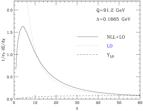
Figure 1: Results to NLL+LO accuracy.

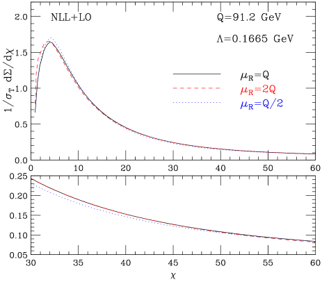
Figure 2: Results to NLL+LO accuracy: scale dependence.

In the following we present quantitative results at NLL+LO and NNLL+NLO accuracy. At NLL+LO the resummed component in Eq. (4) is evaluated by including the functions $g_{1}$ and $g_{2}$ in Eq. (2) and the coefficient $H^{(1)}$ in Eq. (14). The finite component in Eq. (22) is instead evaluated at LO and the one-loop expression for $\alpha_{\mathrm{S}}$ is used. At NNLL+NLO we include also the function $g_{3}$ in the resummed component and we evaluate the finite part at NLO, with $\alpha_{\mathrm{S}}$ at two-loop level.

The NLL+LO results are shown in Figs. 1 and 2. They are obtained by fixing $\Lambda^{n_{F}=5}_{\rm QCD}=0.1665$ GeV, corresponding to $\alpha_{\mathrm{S}}(M_{Z})=0.130$. In Fig. 1 we show the results for $\mu_{R}=Q$. The dotted line is the LO result, which diverges to $+\infty$ as $\chi\rightarrow 0$. The solid line is the matched result, and the dashed line gives the matching term in Eq. (22). Note that we plot $1/\sigma_{T}~{}d\Sigma/d\chi$, so that the matching term is actually $Y(\chi)\equiv 1/\sigma_{T}~{}d\Sigma^{(\rm fin.)}/d\chi$. As can be observed, the matching term is well behaved up to very small values of $\chi$ and becomes dominant at larger $\chi$, where the fixed-order contribution is expected to control the matched calculation.

The scale dependence at NLL+LO is studied in Fig. 2, where the results for the scales $\mu_{R}=Q/2,Q,2Q$ are shown. The lower plot shows the detail of the region $30^{\circ}<\chi<60^{\circ}$.

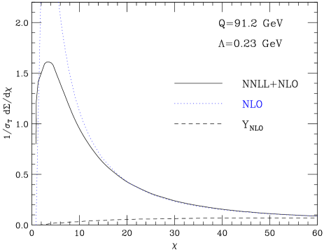
Figure 3: Results to NNLL+NLO accuracy.

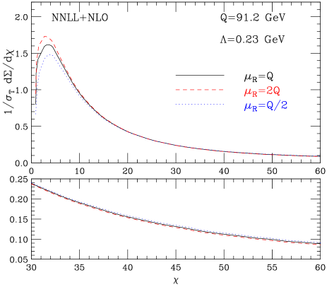
Figure 4: Results to NNLL+NLO accuracy: scale dependence.

The NNLL+NLO results are shown in Figs. 3 and 4. They are obtained using $\Lambda^{n_{F}=5}_{\rm QCD}=0.23$ GeV, corresponding to $\alpha_{\mathrm{S}}(M_{Z})=0.118$. As before, Fig. 3 shows the results for $\mu_{R}=Q$. The dotted line is the NLO contribution, which diverges to $-\infty$ as $\chi\rightarrow 0$. The solid line is the matched result, and the dashed line gives the matching term in Eq. (22). We see that this matching term displays a very smooth behaviour as $\chi\rightarrow 0$, and this is a further confirmation of the validity of our result in Eq. (19). The NNLL+NLO result is plotted in Fig. 4 for $\mu_{R}=Q/2,Q,2Q$. As in Fig. 2, the lower panel shows the detail of the region $30^{\circ}<\chi<60^{\circ}$.

We see that scale variations act differently in the low-$\chi$ and medium-$\chi$ regions. In the region of the peak, lowering (increasing) $\mu_{R}$ has the effect of increasing (lowering) $\alpha_{\mathrm{S}}(\mu_{R})$ and thus increasing (damping) the Sudakov suppression. This results in the fact that, at NNLL+NLO, the curve at $\mu_{R}=2Q$ is higher than the one at $\mu_{R}=Q/2$. This behaviour changes as $\chi$ increases and at $\chi=60^{\circ}$ the curves are in the usual order. At NLL+LO these two distinct features (Sudakov suppression and perturbative increase with $\alpha_{\mathrm{S}}$) are less evident, and thus the scale dependence appears smaller than at NNLL+NLO. At NNLL+NLO the scale dependence is about $\pm 8\%$ at the peak and about $\pm 5\%$ at $\chi=60^{\circ}$, giving an idea of the theoretical uncertainty in the resummed calculation.

We find that the NNLL effect is dominated by the contribution of $B^{(2)}$ in the function $g_{3}$. By keeping only the term proportional to $B^{(2)}$ in the function $g_{3}$ in Eq. (2), the difference with respect to the full NNLL+NLO result is smaller than $1\%$.

Figure 5 shows the NNLL+NLO matched result in the full range of $\chi$. We see that, contrary to what happens in other approaches to $b$-space resummation [32], there are no oscillations in the medium–high $\chi$ region, where the matched result follows the NLO fixed order calculation.

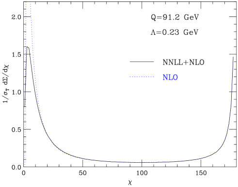
Figure 5: NNLL+NLO results in the full $\chi$ range

Before moving to the comparison with the experimental data, we want to study the convergence of the resummed expression, as a check of the validity of the prescription introduced in [29] and used to deal with the Landau pole. In Fig. 6 we compare the purely resummed result in Eq. (4) at NNLL accuracy (that is with the functions $g_{1}$, $g_{2}$, $g_{3}$ and the coefficient $H^{(1)}$ included) with its expansion up to ${\cal O}(\alpha_{\mathrm{S}}^{6})$. As can be observed, the expansion converges very rapidly to the resummed result in the region of medium $\chi$, confirming the validity of the prescription where the fixed-order result dominates (see the lower plot for a detailed comparison). Nonetheless, even though the higher the expansion the better the agreement with the resummed result at smaller values of $\chi$, for $\chi\raisebox{-1.72218pt}{\hbox to0.0pt{$\,\sim\,$\hss}}\raisebox{1.72218pt}{$\,<\,$}10^{\circ}$ the fixed-order result is bound to fail, no matter how many orders in perturbation theory are included, thus requiring the resummation to all orders.

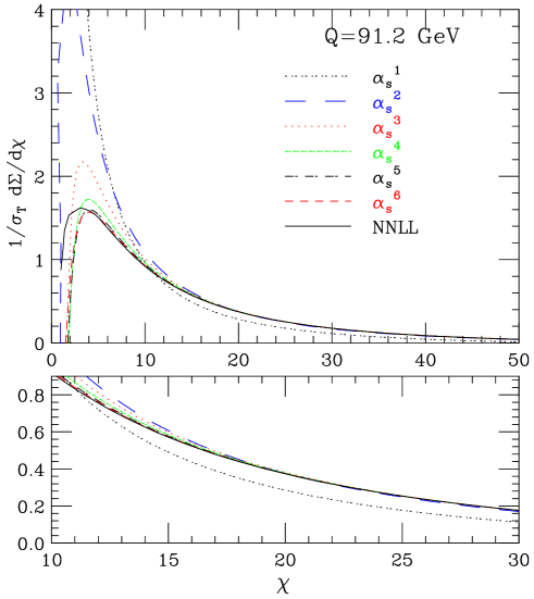
Figure 6: Comparison between the purely resummed and the expanded expression (up to ${\cal O}(\alpha_{\mathrm{S}}^{6})$) for the EEC

We can now perform a comparison of the most accurate theoretical NNLL+NLO results with the precise OPAL [30] and SLD [31] data. As the extraction of the strong coupling constant $\alpha_{\mathrm{S}}$ is one of the main motivations for the measurement of event-shape observables, we perform a fit of the experimental data on EEC leaving $\Lambda_{\rm QCD}$ as a free parameter. We do not attempt to produce the most accurate extraction of $\alpha_{\mathrm{S}}(M_{Z})$, since we cannot properly take into account correlations between the data points and therefore just add systematic and statistical errors in quadrature.

For the moment we neglect hadronization effects, but we will come back to this point below. The reader should keep in mind that the results obtained without including those effects should be considered with care.

In a first sample we include data in the range $15^{\circ}<\chi<120^{\circ}$ and fix the renormalization scale to $\mu_{R}=Q=M_{Z}$. The upper limit is chosen so as to cut the large angle region where another resummation would be required.

The quality of the fit is poor, as can be determined by the value of $\chi^{2}/{\rm d.o.f.}=5.17$, with a rather large value for the coupling constant $\alpha_{\mathrm{S}}(M_{Z})=0.133\pm 0.002$, in agreement with similar results found by OPAL [30]. The uncertainty is dominated by missing higher-order contributions, estimated by repeating the fit with $\mu_{R}=1/2\,(2)M_{Z}$. Better fit results are actually found when the renormalization scale is also varied, with a reduction of a factor of 2 in $\chi^{2}$ when $\mu_{R}\simeq M_{Z}/2$ and a slightly lower preferred value of the coupling constant.

Figure 7: NNLL+NLO: purely PT fit in the low-$\chi$ region

In a second attempt, we include data in the range $0^{\circ}<\chi<63^{\circ}$, to isolate the region where the effects of the resummation are considerably more significant. Even with the scale fixed to $\mu_{R}=M_{Z}$, a very reasonable value of $\chi^{2}/{\rm d.o.f.}=1.67$ is found, corresponding to $\alpha_{\mathrm{S}}(M_{Z})=0.131\pm 0.002$. The error is again dominated by scale variations $\mu_{R}=1/2M_{Z},2M_{Z}$. The nice comparison between the resummed calculation and the data in the low-angle region is shown in Fig. 7. It is clear that our NNLL+NLO result for the EEC can reproduce very well the data up to the lowest measured angle.

Since the low-$\chi$ region is particularly sensitive to non-perturbative (NP) effects, whereas in the large angle region we may expect non negligible higher-order (NNLO) contributions, we have repeated the fit in the range $15^{\circ}<\chi<63^{\circ}$. The value of $\chi^{2}/{\rm d.o.f.}$ goes down to 0.66 but the result for $\alpha_{\mathrm{S}}(M_{Z})$ does not change significantly.

We have also investigated the possible effect of the unknown second-order coefficient $H^{(2)}$ (see Eq. (8)), by letting it vary together with $\alpha_{\mathrm{S}}(M_{Z})$ in the range $0^{\circ}<\chi<63^{\circ}$. The results show that data still prefer a high $\alpha_{\mathrm{S}}(M_{Z})$ and a relatively small $H^{(2)}$.

Up to now we have considered only the perturbative contribution in the theoretical calculation. However, NP contributions are expected to be relevant, particularly for small angles [1, 13, 33]. Thus, following Ref. [21], we include NP effects by supplementing the Sudakov form factor in Eq. (5) with a correction of the form

$$S_{\rm NP}=e^{-\frac{1}{2}a_{1}b^{2}}(1-2a_{2}b)\,.$$ (23)

We have performed a three-parameter preliminary fit to the data still in the range $0^{\circ}<\chi<63^{\circ}$. We find that the data prefer very small values of the NP coefficient $a_{2}$, $|a_{2}|\raisebox{-1.72218pt}{\hbox to0.0pt{$\,\sim\,$\hss}}\raisebox{1.72218pt}{$\,<\,$}0.002$. We have thus set $a_{2}=0$ to perform the fit. We obtain for $\alpha_{\mathrm{S}}(M_{Z})$ and $a_{1}$ the following result:

$$\alpha_{\mathrm{S}}(M_{Z})=0.130^{+0.002}_{-0.004}~{}~{}~{}~{}a_{1}=1.5^{+3.2}_{-0.5}~{}{\rm GeV}^{2}$$ (24)

with $\chi^{2}/{\rm d.o.f.}=0.99$. The error is dominated by scale uncertainty, which is estimated as above by repeating the fit with $\mu_{R}=1/2(2)M_{Z}$.

We see that the quality of the fit improves, but the value of $\alpha_{\mathrm{S}}(M_{Z})$ still remains high with respect to the world average $\alpha_{\mathrm{S}}(M_{Z})=0.1182\pm 0.0027$ [34]. Moreover, the three-parameter fit suggests that in our approach the NP coefficient $a_{1}$ is more important than $a_{2}$. We conclude that the parametrization in Eq. (23) is not able to fully take into account the hadronization effects, particularly at medium and large values of $\chi$. The extracted “effective” coupling $\alpha_{\mathrm{S}}$ thus absorbs part of the hadronization effects. We stress that this result is not an artefact of the resummation procedure, since a similar effect is observed when the large-angle data are compared with the fixed order NLO result.

A different method to include NP (hadronization) corrections, extensively applied in the QCD analysis to event-shape variables at LEP, is to use a parton shower Monte Carlo. This method is certainly model-dependent, since different approaches have been developed to describe the hadronization process, but has the advantage that the free parameters are tuned through fits to large sets of different data.

In Refs. [30, 31] the data for EEC have been corrected at parton level before performing the QCD analysis. We have used the parton-level data of Ref. [30] to repeat our fit. The hadron–parton correction factors are large, from about $1.5$ in the very small $\chi$ region to $\sim 0.9$ at large $\chi$. The quality of the fit in terms of $\chi^{2}/{\rm d.o.f.}$ is generally worse than before, but errors related to the hadronization correction have not been included. The uncertainty from hadronization is usually estimated by trying different alternatives for the hadronization correction, and using the spread in the results as an estimate of the ensuing error. In Ref. [30] the hadronization uncertainty on $\alpha_{\mathrm{S}}(M_{Z})$ is estimated to be about $\pm 4\%$.

In the kinematical range $15^{\circ}<\chi<63^{\circ}$ we find $\chi^{2}/{\rm d.o.f.}=3.78$ and $\alpha_{\mathrm{S}}=0.119\pm 0.001$, with a very similar result ($\chi^{2}/{\rm d.o.f.}=5.02$ and $\alpha_{\mathrm{S}}=0.120\pm 0.001$) when the fit range is extended to $15^{\circ}<\chi<120^{\circ}$. Finally, when the fit is repeated by allowing the variation of the renormalization scale, excellent results are obtained, the best fit corresponding to $\alpha_{\mathrm{S}}=0.1175$, $\chi^{2}/{\rm d.o.f.}=1.36$ and $\mu_{R}=0.28\,M_{Z}$ (see Fig. 8). Thus, when hadronization effects are taken into account using a Monte Carlo, as done in Refs. [30, 31], the results we obtain for $\alpha_{\mathrm{S}}(M_{Z})$ are in complete agreement with the world average.

We note that the QCD analysis performed by OPAL on the same parton-level data gave, instead, $\alpha_{\mathrm{S}}(M_{Z})=0.132^{+0.008}_{-0.007}$ [30], considerably higher than our result.

Figure 8: Comparison of NNLL+NLO fit to parton level OPAL data with $\alpha_{\mathrm{S}}(M_{Z})=0.1175$

The analysis of Ref. [30] (as well as the one of Ref. [31]) used the NLL resummed calculation of Ref. [16]. In order to understand the origin of the discrepancy, we have compared our results with those of Ref. [16]. We find that the differences are not negligible, especially in the region $\chi\raisebox{-1.72218pt}{\hbox to0.0pt{$\,\sim\,$\hss}}\raisebox{1.72218pt}{$\,<\,$}40^{\circ}$, and may explain the above discrepancy. The approach of Ref. [16] was based on an approximated analytic evaluation of the $b$-space integral of Eq. (4), and suffers from an unphysical singularity at very small $\chi$. The effect of this singularity may propagate also within the range of the fit, thus spoiling the resummed prediction. The other source of difference is that the coefficient $B^{(2)}$, or equivalently $G_{21}$, was evaluated numerically, thus leading to a larger uncertainty in the matching procedure.

4 Conclusions

In this paper we have considered the observable known as energy–energy correlation in $e^{+}e^{-}$ collisions. We have provided the complete structure of the ${\cal O}(\alpha_{\mathrm{S}}^{2})$ logarithmically enhanced contributions up to NNLL accuracy, by giving the expression of the unknown second-order coefficient $B^{(2)}$, needed to reach full NNLL precision.

We have presented perturbative predictions both at NLL+LO and NNLL+NLO accuracy, by showing that the knowledge of the calculated coefficient $B^{(2)}$ allows us to perform an excellent matching of the resummed and fixed-order calculations. We have studied the impact of the results in a detailed comparison to precise LEP and SLC data. A good description of the data is obtained but the extracted value of $\alpha_{\mathrm{S}}(M_{Z})$ turns out to be high when hadronization effects are neglected or parametrized using the form in Eq. (23). By contrast, using OPAL data corrected at parton level, that were obtained by estimating hadronization corrections using a Monte Carlo parton shower, the values of $\alpha_{\mathrm{S}}(M_{Z})$ we find are in good agreement with the current world average.

Acknowledgements

We would like to thank Stefano Catani for many helpful discussions and suggestions. We also thank Mrinal Dasgupta, Lance Dixon, Luca Trentadue and Bryan Webber for useful discussions and comments. We are grateful to David Ward and the OPAL collaboration for providing us the parton-level data used in the analysis.

References

- [1] C. L. Basham, L. S. Brown, S. D. Ellis and S. T. Love, Phys. Rev. Lett. 41 (1978) 1585.
- [2] D. G. Richards, W. J. Stirling and S. D. Ellis, Phys. Lett. B 119 (1982) 193 and 136 (1984) 99, Nucl. Phys. B 229 (1983) 317.
- [3] S. C. Chao, D. E. Soper and J. C. Collins, Nucl. Phys. B 214 (1983) 513.
- [4] H. N. Schneider, G. Kramer and G. Schierholz, Z. Phys. C 22 (1984) 201.
- [5] A. Ali and F. Barreiro, Phys. Lett. B 118 (1982) 155.
- [6] Z. Kunszt and P. Nason in “Z Physics at LEP 1” CERN 89-08 (CERN, Geneva, 1989), Vol 1, p.373.
- [7] N. K. Falck and G. Kramer, Z. Phys. C 42 (1989) 459.
- [8] E. W. Glover and M. R. Sutton, Phys. Lett. B 342 (1995) 375.
- [9] K. A. Clay and S. D. Ellis, Phys. Rev. Lett. 74 (1995) 4392.
- [10] G. Kramer and H. Spiesberger, Z. Phys. C 73 (1997) 495.
- [11] S. Catani and M. H. Seymour, Phys. Lett. B 378 (1996) 287, Nucl. Phys. B 485 (1997) 291 [Erratum-ibid. B 510 (1997) 503].
- [12] See also P. Nason et al., in “Physics at LEP2”, CERN 96-01 (CERN, Geneva 1996), vol. 1 p. 246.
- [13] J. C. Collins and D. E. Soper, Nucl. Phys. B 193 (1981) 381 [Erratum-ibid. B 213 (1983) 545]; Nucl. Phys. B 197 (1982) 446; Nucl. Phys. B 284 (1987) 253.
- [14] J. Kodaira and L. Trentadue, Phys. Lett. B 112 (1982) 66 and 123 (1983) 335.
- [15] D. de Florian and M. Grazzini, Phys. Rev. Lett. 85 (2000) 4678, Nucl. Phys. B 616 (2001) 247.
- [16] G. Turnock, report CAVENDISH-HEP-92-3.
- [17] S. Frixione, P. Nason and G. Ridolfi, Nucl. Phys. B 542 (1999) 311.
- [18] S. Catani, D. de Florian and M. Grazzini, Nucl. Phys. B 596 (2001) 299.
- [19] S. Moch, J. A. M. Vermaseren and A. Vogt, Nucl. Phys. B 688 (2004) 101.
- [20] A. Vogt, S. Moch and J. A. M. Vermaseren, hep-ph/0404111.
- [21] Y. L. Dokshitzer, G. Marchesini and B. R. Webber, JHEP 9907 (1999) 012.
- [22] A. Bassetto, M. Ciafaloni and G. Marchesini, Phys. Rep. 100 (1983) 201, and references therein.
-
[23]
J.M. Campbell and E.W.N. Glover, Nucl. Phys. B 527 (1998) 264;
S. Catani and M. Grazzini, Phys. Lett. B 446 (1999) 143, Nucl. Phys. B 570 (2000) 287;
V. Del Duca, A. Frizzo and F. Maltoni, Nucl. Phys. B 568 (2000) 211. -
[24]
Z. Bern, L. Dixon, D.C. Dunbar and D.A. Kosower, Nucl. Phys. B 425
(1994) 217;
Z. Bern and G. Chalmers, Nucl. Phys. B 447 (1995) 465;
Z. Bern, V. Del Duca, W.B. Kilgore and C.R. Schmidt, Phys. Rev. D 60 (1999) 116001;
D.A. Kosower and P. Uwer, Nucl. Phys. B 563 (1999) 477;
S. Catani and M. Grazzini, Nucl. Phys. B 591 (2000) 435. - [25] G. Curci, W. Furmanski and R. Petronzio, Nucl. Phys. B 175 (1980) 27.
- [26] W. Furmanski and R. Petronzio, Phys. Lett. B 97 (1980) 437.
- [27] L. Dixon, private communication.
- [28] G. Bozzi, S. Catani, D. de Florian and M. Grazzini, Phys. Lett. B 564 (2003) 65.
- [29] E. Laenen, G. Sterman and W. Vogelsang, Phys. Rev. Lett. 84 (2000) 4296; A. Kulesza, G. Sterman and W. Vogelsang, Phys. Rev. D 66 (2002) 014011.
- [30] D. Acton et al. [OPAL Collaboration], Z. Phys. C 59 (1993) 1.
- [31] K. Abe et al. [SLD Collaboration], Phys. Rev. D 51 (1995) 962.
- [32] See e.g. P. B. Arnold and R. P. Kauffman, Nucl. Phys. B 349 (1991) 381.
- [33] R. Fiore, A. Quartarolo and L. Trentadue, Phys. Lett. B 294 (1992) 431.
- [34] S. Bethke, hep-ex/0407021, talk given at the 7th DESY Workshop on Elementary Particle Theory, “Loops and Legs in Quantum Field Theory”, Zinnowitz, Germany, 2004.