IFIC/04$-$06

FTUV/04$-$0721

Quantum Loops in the Resonance Chiral Theory:
The Vector Form Factor
I. Rosell, J.J. Sanz-Cillero and A. Pich

Departament de Física Teòrica, IFIC, Universitat de València - CSIC
Apt. Correus 22085, E-46071 València, Spain

We present a calculation of the Vector Form Factor at the next-to-leading order in the $1/N_{C}$ expansion, within the framework of Resonance Chiral Theory. The calculation is performed in the chiral limit, and with two dynamical quark flavours. The ultraviolet behaviour of quantum loops involving virtual resonance propagators is analyzed, together with the kind of counterterms needed in the renormalization procedure. Using the lowest-order equations of motion, we show that only a few combinations of local couplings appear in the final result. The low-energy limit of our calculation reproduces the standard Chiral Perturbation Theory formula, allowing us to determine the resonance contribution to the chiral low-energy couplings, at the next-to-leading order in $1/N_{C}$, keeping a full control of their renormalization scale dependence.

1 Introduction

We have at present an overwhelming experimental and theoretical evidence that the $SU(3)_{C}$ gauge theory correctly describes the hadronic world [1]. This makes QCD the established theory of the strong interactions. Nevertheless, its non-perturbative nature at long distances is still challenging our theoretical capabilities. Since the hadronization procedure is not understood, an effective field theory description [2] in terms of hadronic degrees of freedom is required in the low-energy regime.

Below the heavy quark thresholds, QCD is properly described considering only the light quarks, with masses much smaller than the dynamical QCD scale $\Lambda_{QCD}$. One can then study the massless QCD case and consider the mass term as a perturbation. With $n_{f}$ massless quarks, QCD has a chiral $SU(n_{f})_{R}\otimes SU(n_{f})_{L}$ symmetry which is spontaneously broken to $SU(n_{f})_{L+R}$. This generates $(n_{f}^{2}-1)$ Goldstone bosons, which can be identified with the multiplet of light pseudoscalars; their small masses being proportional to the explicit breaking of chiral symmetry generated by the quark masses. The Goldstone nature of the pseudoscalar bosons implies strong constraints on their interactions, which can be most easily analyzed on the basis of an effective Lagrangian organized as an expansion in powers of momenta (derivatives) and quark masses over the chiral symmetry breaking scale $\Lambda_{\chi}\simeq 4\pi F_{\pi}\simeq 1.2$ GeV. The resulting Goldstone effective field theory, Chiral Perturbation Theory ($\chi$PT) [3, 4, 5], has achieved a remarkable success describing the low-energy dynamics of QCD [6, 7].

In the resonance region one must introduce a different effective field theory with explicit massive fields to describe the degrees of freedom associated with the mesonic resonances [8, 9]. Although chiral symmetry still provides stringent dynamical constraints, the usual $\chi$PT power counting breaks down in the presence of higher energy scales. Therefore, one needs another expansion parameter to organize the effective Lagrangian. The limit of an infinite number of quark colours [10] turns out to be a very useful tool to understand many features of QCD and provides an alternative power counting to describe the meson interactions [11]. Taking $N_{C}\to\infty$, with $\alpha_{s}N_{C}$ fixed, there exists a systematic expansion of the $SU(N_{C})$ gauge theory in powers of $1/N_{C}$, which for $N_{C}=3$ provides a good quantitative approximation scheme to the hadronic world [12]. Assuming confinement, the strong dynamics at $N_{C}\to\infty$ is given by tree diagrams with infinite sums of hadron exchanges, which correspond to the tree approximation to some local effective Lagrangian. Hadronic loops generate corrections suppressed by factors of $1/N_{C}$.

The short-distance properties of the underlying QCD dynamics impose strong constraints on the couplings of the hadronic effective theory [9, 11]. The infinite sums of meson exchanges contributing to any given Green function should obey the right QCD behaviour $G(t)\sim t^{\omega}$ at large momenta. This requirement excludes resonance interactions with large number of derivatives, explaining the phenomenological success of the usual lowest-order (in derivatives) approximations. Moreover, it implies stringent correlations among those resonance couplings associated with the highest powers of momenta. The usual $\chi$PT expansion is of course recovered at very low energies, when the resonance Green functions are expanded in powers of momenta over the resonance mass scale.

In spite of its many dynamical simplifications, QCD at $N_{C}\to\infty$ is still a very involved theory and some approximations are called for. Usually one cuts the infinite tower of resonance exchanges to a finite number, taking only into account those meson states which are relevant at the physical energy scale. This is meaningful since the contributions from higher-mass states are suppressed by their corresponding propagators. However, it introduces back a momentum expansion regulated by inverse powers of the heavier resonance masses which have been integrated out. The problem can be formally avoided taking the limit $M_{R}\to\infty$ for all resonance states not included in the effective theory. This gives a well-defined approximation with a clear physical meaning: one is assuming that the QCD short-distance operator product expansion provides an acceptable description at energies above the last included mesonic state. The imposed short-distance constraints are nothing else than matching conditions between the low-energy effective field theory and the underlying QCD dynamics.

The most drastic and simplest scheme is the so-called Single Resonance Approximation, which only considers the contributions from the lightest meson with any given quantum numbers [8, 9, 13, 14]. The short-distance QCD constraints determine in this case all hadronic parameters in terms of the pion decay constant $F_{\pi}$ and the two masses of the vector and scalar multiplets, $M_{V}$ and $M_{S}$ [11]. This gives a very successful description at energies below the scale of the second resonance multiplets. Since there is an infinite number of Green functions, it is clearly not possible to satisfy all matching conditions within the single resonance approximation. A useful generalization is the Minimal Hadronic Ansatz, which keeps the minimum number of resonances compatible with all known short-distance constraints for the problem at hand [15]. The resonance contributions to some ${\cal O}(p^{6})$ $\chi$PT couplings have been already analyzed in this way, by studying an appropriate set of three-point functions [16, 17, 18].

The $N_{C}\to\infty$ limit of the resonance chiral theory (R$\chi$T) has been investigated in many works [8, 9, 11, 13, 14, 15, 16, 17, 18] and a very successful leading order phenomenology already exists [11]. However, we are still lacking a systematic procedure to incorporate next-to-leading contributions in the $1/N_{C}$ counting. Up to now, the effort has concentrated in pinning down the most relevant subleading effects, such as the resonance widths which regulate the corresponding poles in the meson propagators [19, 20, 21], or the role of final state interactions in the physical amplitudes [19, 20, 21, 22, 23, 24, 25, 26, 27]. These unitarity corrections are generated through Goldstone loops and therefore are suppressed by $1/N_{C}$ factors; nevertheless they may be strongly enhanced by large infrared logarithms. The combined constraints of analyticity and unitarity make possible to perform appropriate resummations of chiral logarithms, which describe the leading $1/N_{C}$ corrections in the resonance region.

Quantum loops including virtual resonance propagators are a major technical challenge which has never been properly addressed. A first step in this direction was the study of resonance loop contributions to the running of the $\chi$PT coupling $L_{10}(\mu)$, performed in Ref. [28], which however didn’t attempt any analysis of the induced ultraviolet divergences and their corresponding renormalization. Clearly, at the one-loop level the massive states present in R$\chi$T generate all kind of ultraviolet problems which are not yet understood. A naive chiral power counting indicates that the renormalization procedure will require higher dimensional counterterms, which presumably could generate a problematic behaviour at large momenta. Therefore, it will be necessary to perform a careful investigation of the constraints implied by the short-distance properties of QCD at the next-to-leading order in $1/N_{C}$.

A formal renormalization of R$\chi$T at the one-loop level appears to be a very involved task, which requires the prior analysis of several technical ingredients [34]. In order to gain some understanding on the ultraviolet behaviour, it seems worth to perform first some explicit one-loop calculations of well chosen physical amplitudes. In the following, we present a detailed investigation of the pion vector form factor (VFF) at the next-to-leading order (NLO) in the $1/N_{C}$ expansion. This observable is defined through the two-Goldstone matrix element of the vector current:

$$\langle\,\pi^{+}(p_{1})\,\pi^{-}(p_{2})\,|\,\frac{\displaystyle 1}{\displaystyle 2}\left(\bar{u}\gamma^{\mu}u-\bar{d}\gamma^{\mu}d\right)\,|0\rangle\,=\,\mathcal{F}(q^{2})\,(p_{1}-p_{2})^{\mu}\,,$$ (1)

where $q^{\mu}\equiv(p_{1}+p_{2})^{\mu}$. At very low energies, the VFF $\mathcal{F}(q^{2})$ has been studied within the $\chi$PT framework up to ${\cal O}(p^{6})$ [35, 36, 37]. R$\chi$T and the $1/N_{C}$ expansion have been also used to determine $\mathcal{F}(q^{2})$ at the $\rho$ meson peak, including appropriate resummations of subleading infrared logarithms [19, 20, 21, 22].

We will simplify the calculation working in the two flavour theory and taking the massless quark limit. Therefore, we will assume a chiral $U(2)_{L}\otimes U(2)_{R}$ symmetry group. The small effects induced by the $U(1)_{A}$ anomaly will be neglected, because they are not going to be relevant in our discussion. The isosinglet pseudoscalar can only appear within loops, and the numerical correction generated by its non-zero mass could be taken into account in a straightforward way, together with the finite quark mass effects which we are ignoring.

In the next section we will briefly describe the R$\chi$T Lagrangian. We will adopt the single resonance approximation and will only consider the minimal set of resonance couplings (linear in the resonance fields) introduced in ref. [8], supplemented with those counterterms required by the renormalization procedure. The renormalization of the relevant one-particle-irreducible Feynman diagrams will be discussed in section 3 and the final results of our calculation will be collected in section 4. Sections 5 and 6 analyze the behaviour of the computed vector form factor at low and high energies, respectively. We will finally summarize our findings in section 7. Some technical details have been relegated to the appendices.

2 The Lagrangian of Resonance Chiral Theory

We are going to work within a $U(2)_{L}\otimes U(2)_{R}$ chiral theory, containing a multiplet of 4 pseudoscalar Goldstone bosons,

$$\Phi\,=\,\pmatrix{{1\over\sqrt{2}}\pi^{0}+{1\over\sqrt{2}}\eta_{0}&\pi^{+}\cr\pi^{-}&-{1\over\sqrt{2}}\pi^{0}+{1\over\sqrt{2}}\eta_{0}}\,,$$ (2)

parameterized through the unitary matrix  $u(\Phi)=\exp{\left\{i\,\Phi/(\sqrt{2}\,F)\right\}}$. The Goldstones couple to massive $U(2)$ multiplets of the type $V(1^{--})$, $A(1^{++})$, $S(0^{++})$ and $P(0^{-+})$, with a field content analogous to the one indicated in (2).

Our starting point is the R$\chi$T Lagrangian $\mathcal{L}(u,V,A,S,P)$ introduced in Ref. [8]. It contains the ${\cal O}(p^{2})$ $\chi$PT Lagrangian [4, 5],

$$\mathcal{L}_{2\chi}\,=\,\frac{\displaystyle F^{2}}{\displaystyle 4}\,\langle\,u_{\mu}u^{\mu}\,+\,\chi_{+}\,\rangle\,,$$ (3)

the kinetic resonance Lagrangians,

$$\begin{array}[]{ccl}\mathcal{L}_{2Z}(R=V,A)&=&-{1\over 2}\,\langle\nabla^{\lambda}R_{\lambda\mu}\nabla_{\nu}R^{\nu\mu}-{1\over 2}\,M^{2}_{R}\,R_{\mu\nu}R^{\mu\nu}\rangle\,,\\ \\ \mathcal{L}_{2Z}(R=S,P)&=&{1\over 2}\,\langle\nabla^{\mu}R\,\nabla_{\mu}R-M^{2}_{R}\,R^{2}\rangle\,,\end{array}$$ (4)

and ${\cal O}(p^{2})$ interactions linear in the resonance fields:

$$\begin{array}[]{ccl}\mathcal{L}_{2V}[V(1^{--})]&=&\frac{\displaystyle F_{V}}{\displaystyle 2\sqrt{2}}\,\langle V_{\mu\nu}f_{+}^{\mu\nu}\rangle\,+\,\frac{\displaystyle i\,G_{V}}{\displaystyle 2\sqrt{2}}\,\langle V_{\mu\nu}\left[u^{\mu},u^{\nu}\right]\rangle\,,\\ \\ \mathcal{L}_{2A}[A(1^{++})]&=&\frac{\displaystyle F_{A}}{\displaystyle 2\sqrt{2}}\,\langle A_{\mu\nu}f_{-}^{\mu\nu}\rangle\,,\\ \\ \mathcal{L}_{2S}[S(0^{++})]&=&c_{d}\,\langle S\,u_{\mu}u^{\mu}\rangle\,+\,c_{m}\,\langle S\,\chi_{+}\rangle\,,\\ \\ \mathcal{L}_{2P}[P(0^{-+})]&=&i\,d_{m}\,\langle P\,\chi_{-}\rangle\,.\end{array}$$ (5)

The brackets $\langle\,...\,\rangle$ denote a trace of the corresponding flavour matrices, and the different chiral tensors follow the notation defined in Ref. [8]. They include external vector, axial-vector, scalar and pseudoscalar sources ($v^{\mu}$, $a^{\mu}$, $s$, $p$) to generate the corresponding Green functions. Following this reference, we describe the vector and axial-vector resonances with the antisymmetric field formalism. In the chiral limit and neglecting external scalar or pseudoscalar sources $\chi_{\pm}=0$.

The Lagrangian $\mathcal{L}(u,V,A,S,P)$ obeys the correct $N_{C}$ counting rules. The different fields and the masses and momenta are all of them ${\cal O}(1)$, whereas all couplings ($F$, $F_{V}$, $G_{V}$, $F_{A}$, $c_{d}$, $c_{m}$ and $d_{m}$) are of ${\cal O}\left(\sqrt{N_{C}}\,\right)$. In the limit $N_{C}\to\infty$, one can determine all parameters in terms of $F$, $M_{V}$ and $M_{S}$ [11]. The short-distance QCD behaviour of the vector, axial-vector [9] and scalar [24] form factors, together with the constraints implied [9, 11, 14] by the superconvergence properties of the $vv-aa$ [38] and $ss-pp$ two-point functions at large momenta, imply the relations [11]:

$${F_{V}\over\sqrt{2}}=\sqrt{2}\,G_{V}=F_{A}=2\,c_{m}=2\,c_{d}=2\sqrt{2}\,d_{m}=F\,,$$ (6)

$$M_{A}=\sqrt{2}\,M_{V}\qquad,\qquad M_{P}=\sqrt{2}\,M_{S}\,\left(1-\delta\right)^{1/2}\,.$$ (7)

The last identity involves a small correction  $\delta\approx 3\,\pi\alpha_{s}F^{2}/M_{S}^{2}\sim 0.08\,\alpha_{s}$, which can be neglected together with the tiny effects from light quark masses.

2.1 Subleading Lagrangian

The one loop calculation of the VFF with the previous Lagrangian generates ultraviolet divergences which require counterterms with a higher number of derivatives. We will only include the minimal set of chiral structures needed to renormalize the VFF calculation. We expect their corresponding couplings to be subleading in the $1/N_{C}$ expansion, since they are associated with quantum loop corrections.

We need to include the following ${\cal O}(p^{4})$ and ${\cal O}(p^{6})$ Goldstone interactions:

$$\widetilde{\mathcal{L}}_{4\chi}\,=\,\frac{\displaystyle i\,\widetilde{\ell}_{6}}{\displaystyle 4}\,\langle\,f_{+}^{\mu\nu}\left[u_{\mu},u_{\nu}\right]\,\rangle\,-\,\widetilde{\ell}_{12}\,\langle\,\nabla^{\mu}u_{\mu}\nabla^{\nu}u_{\nu}\,\rangle\,,$$ (8)

$$\widetilde{\mathcal{L}}_{6\chi}\,=\,i\,\widetilde{c}_{51}\,\langle\,\nabla^{\rho}f_{+}^{\mu\nu}[h_{\mu\rho},u_{\nu}]\,\rangle\,+\,i\,\widetilde{c}_{53}\,\langle\,\nabla_{\mu}f_{+}^{\mu\nu}[h_{\nu\rho},u^{\rho}]\,\rangle\,.$$ (9)

Chiral invariance forces these terms to have structures contained in the corresponding $\chi$PT Lagrangians [4, 39]. We use a tilde to denote the R$\chi$T couplings in (8) and (9), which are different to the ones with the same names (without tilde) in $\chi$PT. For instance, the $\chi$PT coupling $\ell_{6}$ ($L_{9}$ in the three flavour case) is dominated by a contribution from vector-meson exchange and is of ${\cal O}(N_{C})$, while the corresponding R$\chi$T coupling $\widetilde{\ell}_{6}$ does not contain this contribution and is of ${\cal O}(1)$.

Figure 1: Leading order contributions to the VFF.

The ${\cal O}(p^{4})$ term containing the structure $\nabla^{\mu}u_{\mu}$ does not contribute to the tree–level calculation of the VFF; nevertheless, it is needed to renormalize the Goldstone self-energies. At ${\cal O}(p^{6})$, only the combination of couplings $\widetilde{r}^{\phantom{\,r}}_{V2}\equiv 4F^{2}\,(\widetilde{c}_{53}-\widetilde{c}_{51})$ is going to be relevant for the VFF [39]. Including the Lagrangians (8) and (9), the tree level calculation of the VFF gives the result:

$$\mathcal{F}(q^{2})\,=\,1\,+\,{F_{V}\,G_{V}\over F^{2}}\,{q^{2}\over M_{V}^{2}-q^{2}}\,-\,\widetilde{\ell}_{6}\,{q^{2}\over F^{2}}\,+\,\widetilde{r}^{\phantom{\,r}}_{V2}\,{q^{4}\over F^{4}}\,.$$ (10)

The requirement that the VFF should vanish at $q^{2}\to\infty$ implies the following conditions at leading order in $1/N_{C}$:

$$F_{V}\,G_{V}\,=\,F^{2}\qquad,\qquad\widetilde{\ell}_{6}\,=\,0\qquad,\qquad\widetilde{r}^{\phantom{\,r}}_{V2}\,\equiv\,4F^{2}\,(\widetilde{c}_{53}-\widetilde{c}_{51})\,=\,0\,.$$ (11)

Therefore, the couplings $\widetilde{\ell}_{6}/F^{2}$ and $\widetilde{r}^{\phantom{\,r}}_{V2}/F^{4}$ are of subleading order in the $1/N_{C}$ expansion, i.e. ${\cal O}(1/N_{C})$, as expected on pure dimensional grounds.

The renormalization of Green functions including resonance fields forces the presence of the following additional counterterms:

$$\begin{array}[]{rl}\mathcal{L}_{4Z}\,=&\frac{\displaystyle X_{Z_{1}}}{\displaystyle 2}\,\langle\,\nabla^{2}V^{\mu\nu}\left\{\nabla_{\nu},\nabla^{\sigma}\right\}V_{\mu\sigma}\,\rangle\,+\,\frac{\displaystyle X_{Z_{2}}}{\displaystyle 4}\,\langle\,\left\{\nabla_{\nu},\nabla_{\alpha}\right\}V^{\mu\nu}\left\{\nabla^{\sigma},\nabla^{\alpha}\right\}V_{\mu\sigma}\,\rangle\\ \\ &\mbox{}+\,\frac{\displaystyle X_{Z_{3}}}{\displaystyle 4}\,\langle\,\left\{\nabla^{\sigma},\nabla^{\alpha}\right\}V^{\mu\nu}\left\{\nabla_{\nu},\nabla_{\alpha}\right\}V_{\mu\sigma}\,\rangle\,,\end{array}$$ (12)

$$\mathcal{L}_{4F}\,=\,X_{F_{1}}\,\langle\,V_{\mu\nu}\nabla^{2}f_{+}^{\mu\nu}\,\rangle\,+\,X_{F_{2}}\,\langle\,V_{\mu\nu}\left\{\nabla^{\mu},\nabla_{\alpha}\right\}f_{+}^{\alpha\nu}\,\rangle\,,$$ (13)

$$\mathcal{L}_{4G}\,=\,i\,X_{G_{1}}\,\langle\,\left\{\nabla^{\alpha},\nabla_{\mu}\right\}V^{\mu\nu}\left[u_{\nu},u_{\alpha}\right]\,\rangle\,+\,i\,X_{G_{2}}\,\langle\,V^{\mu\nu}\left[h_{\alpha\mu},h^{\alpha}_{\nu}\right]\,\rangle\,.$$ (14)

The quadratic Lagrangian $\mathcal{L}_{4Z}$ is needed to renormalize the vector self-energy. Actually, only the sum of couplings  $X_{Z}\equiv X_{Z_{1}}+X_{Z_{2}}+X_{Z_{3}}$  is relevant for this purpose. The renormalization of the $v$–$V$ two-point function involves the sum of $\mathcal{L}_{4F}$ couplings  $X_{F}\equiv X_{F_{1}}+X_{F_{2}}$. Finally, the three-point function with one external vector resonance and two Goldstone legs is renormalized by $\mathcal{L}_{4G}$ through the combination  $X_{G}\equiv X_{G_{2}}-\frac{\displaystyle 1}{\displaystyle 2}X_{G_{1}}$. The dimensions of the couplings are $[X_{Z}]=E^{-2}$ and $[X_{F}]=[X_{G}]=E^{-1}$.

At the NLO in $1/N_{C}$, these counterterm Lagrangians only contribute through tree-level diagrams. One can then use the leading order equation of motion (EOM)

$$\begin{array}[]{rl}\nabla^{\mu}\nabla_{\rho}V^{\rho\nu}-\nabla^{\nu}\nabla_{\rho}V^{\rho\mu}\,=&\,-M_{V}^{2}\,V^{\mu\nu}\,-\,\frac{\displaystyle F_{V}}{\displaystyle\sqrt{2}}\,f_{+}^{\mu\nu}\,-\,\frac{\displaystyle iG_{V}}{\displaystyle\sqrt{2}}\,\left[u^{\mu},u^{\nu}\right]\end{array}$$ (15)

to reduce the number of relevant operators. The Lagrangians (12), (13) and (14) take then the equivalent forms:

$$\begin{array}[]{rl}\mathcal{L}_{4Z}^{\mathrm{EOM}}\,=&\frac{\displaystyle X_{Z}M_{V}^{4}}{\displaystyle 2}\,\langle\,V^{\mu\nu}V_{\mu\nu}\,\rangle\,+\,\frac{\displaystyle X_{Z}M_{V}^{2}F_{V}}{\displaystyle\sqrt{2}}\,\langle\,V_{\mu\nu}f_{+}^{\mu\nu}\,\rangle\,+\,\frac{\displaystyle i\,X_{Z}M_{V}^{2}G_{V}}{\displaystyle\sqrt{2}}\,\langle\,V_{\mu\nu}\left[u^{\mu},u^{\nu}\right]\,\rangle\\ \\ &\mbox{}+\,\frac{\displaystyle i\,X_{Z}F_{V}G_{V}}{\displaystyle 2}\,\langle\,f_{+}^{\mu\nu}\left[u_{\mu},u_{\nu}\right]\,\rangle\,+\,\cdots\,,\end{array}$$ (16)

$$\mathcal{L}_{4F}^{\mathrm{EOM}}\,=\,-X_{F}M_{V}^{2}\,\langle\,V_{\mu\nu}f_{+}^{\mu\nu}\,\rangle\,-\,\frac{\displaystyle i\,X_{F}G_{V}}{\displaystyle\sqrt{2}}\,\langle\,f^{\mu\nu}_{+}\left[u_{\mu},u_{\nu}\right]\,\rangle\,+\,\cdots\,,$$ (17)

$$\mathcal{L}_{4G}^{\mathrm{EOM}}\,=\,-2i\,X_{G}M_{V}^{2}\,\langle\,V^{\alpha\nu}\left[u_{\alpha},u_{\nu}\right]\,\rangle\,-\,i\,\sqrt{2}\,X_{G}F_{V}\,\langle\,f_{+}^{\mu\nu}\left[u_{\mu},u_{\nu}\right]\,\rangle\,+\,\cdots\,,$$ (18)

where the dots denote other terms which are not relevant for the VFF calculation at this order. The derivatives acting on the vector resonance fields have been traded by the heavy mass scale $M_{V}$ and/or derivatives acting on the Goldstone fields, giving rise to the usual tensor structures of the $\chi$PT Lagrangian. Therefore, the effect of the counterterm Lagrangians $\mathcal{L}_{4Z}$, $\mathcal{L}_{4F}$ and $\mathcal{L}_{4G}$ is just equivalent to the following shift in the couplings at the next-to-leading order in $1/N_{C}$:

$$\begin{array}[]{rl}\widetilde{\ell}_{6}^{\,\mathrm{eff}}\,=&\widetilde{\ell}_{6}\,+\,2\,X_{Z}F_{V}G_{V}\,-\,2\sqrt{2}\,X_{F}G_{V}\,-\,4\sqrt{2}\,X_{G}F_{V}\,,\\ \\ F_{V}^{\,\mathrm{eff}}\,=&F_{V}\,+\,2\,X_{Z}M_{V}^{2}F_{V}\,-\,2\sqrt{2}\,X_{F}M_{V}^{2}\,,\\ \\ G_{V}^{\,\mathrm{eff}}\,=&G_{V}\,+\,2\,X_{Z}M_{V}^{2}G_{V}\,-\,4\sqrt{2}\,X_{G}M_{V}^{2}\,,\\ \\ (M_{V}^{2})^{\mathrm{eff}}\,=&M_{V}^{2}\,+\,2\,X_{Z}M_{V}^{4}\,,\\ \\ \widetilde{r}^{\,\mathrm{eff}}_{V2}\,=&\widetilde{r}^{\phantom{\,r}}_{V2}\,.\end{array}$$ (19)

Thus, since $\widetilde{\ell}_{6}^{\,\mathrm{eff}}\sim\widetilde{\ell}_{6}\sim(M_{V}^{2})^{\mathrm{eff}}\sim M_{V}^{2}\sim{\cal O}(1)$ and $F_{V}^{\,\mathrm{eff}}\sim F_{V}\sim G_{V}^{\,\mathrm{eff}}\sim G_{V}\sim{\cal O}(\sqrt{N_{C}})$, a consistent $1/N_{C}$ counting requires that $X_{G}$ and $X_{F}$ are of ${\cal O}(1/\sqrt{N_{C}})$ and $X_{Z}$ of ${\cal O}(1/N_{C})$.

3 Renormalization of Quantum Loops

The renormalization procedure follows very systematic and precise steps in any well defined field theory. First of all, the two-point Green functions must be renormalized. Later the three-point Green functions and so on. For the VFF up to NLO in $1/N_{C}$ only the two- and three-point Green functions will contribute. The corresponding renormalizations for the one particle irreducible diagrams (1PI) at one loop are given in the next subsections.

We will adopt the $\overline{MS}-1$ scheme, usually employed in $\chi$PT calculations, where one subtracts the divergent constant

$$\lambda_{\infty}\,=\,\frac{2\,\mu^{d-4}}{d-4}+\gamma_{E}-\ln{4\pi}-1\,.$$ (20)

However, we will impose the on-shell condition to renormalize the pion self-energy. This simplifies the calculation of physical amplitudes with external pions. Since we work in the massless quark limit, the Goldstone tadpoles will not give any contribution. The precise definition of the relevant Feynman integrals with one, two and three propagators and some useful antisymmetric formalism technology are relegated to appendices A and B.

3.1 Pion self-energy

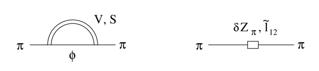
Figure 2: One-loop diagrams and local contributions to the pion self-energy.

The diagrams contributing to the pion propagator are shown in Fig. 2. The kinetic Lagrangians $\mathcal{L}_{2Z}(R)$ in Eq. (4) generate additional tadpole topologies with one resonance propagator, but they are identically zero even with massive pions. The divergences of ${\cal O}(p^{2})$ are reabsorbed through the wave-function renormalization  $\pi^{(B)}=(1+\delta Z_{\pi})^{\frac{1}{2}}\,\pi^{(r)}$, being $\pi^{(B)}$ and $\pi^{(r)}$ the bare and renormalized pion fields respectively. In the on-shell scheme,

$$\delta Z_{\pi}\,=\,-\frac{\displaystyle 2\,G_{V}^{2}}{\displaystyle F^{2}}\,\frac{\displaystyle 3\,M_{V}^{2}}{\displaystyle 16\pi^{2}F^{2}}\,\left\{\lambda_{\infty}+\ln{\frac{\displaystyle M_{V}^{2}}{\displaystyle\mu^{2}}}+\frac{\displaystyle 1}{\displaystyle 6}\right\}\,+\,\frac{\displaystyle 4\,c_{d}^{2}}{\displaystyle F^{2}}\,\frac{\displaystyle M_{S}^{2}}{\displaystyle 16\pi^{2}F^{2}}\,\left\{\lambda_{\infty}+\ln{\frac{\displaystyle M_{S}^{2}}{\displaystyle\mu^{2}}}-\frac{\displaystyle 1}{\displaystyle 2}\right\}\,.$$ (21)

There are also divergences of ${\cal O}(p^{4})$ which renormalize one of the couplings in $\widetilde{\mathcal{L}}_{4\chi}$:

$$\widetilde{\ell}_{12}\,\equiv\,\widetilde{\ell}_{12}^{r}(\mu)+\delta\widetilde{\ell}_{12}(\mu)\qquad\quad;\qquad\quad\delta\widetilde{\ell}_{12}(\mu)\,=\,-\frac{\displaystyle G_{V}^{2}+2\,c_{d}^{2}}{\displaystyle F^{2}}\;\frac{\displaystyle\lambda_{\infty}}{\displaystyle 32\pi^{2}}\;.$$ (22)

The renormalized pion self-energy takes the form

$$-i\,\Sigma_{\pi}^{r}(p^{2}) = -i\,{p^{4}\over 16\pi^{2}F^{2}}\,\left\{64\pi^{2}\,\widetilde{\ell}_{12}^{r}(\mu)\,+\,\frac{\displaystyle 2\,G_{V}^{2}}{\displaystyle F^{2}}\left[\ln{\frac{\displaystyle M_{V}^{2}}{\displaystyle\mu^{2}}}+\phi\left(\frac{\displaystyle p^{2}}{\displaystyle M_{V}^{2}}\right)\right]\right.$$ (23)

$$\left.\hskip 56.9055pt\mbox{}+\,\frac{\displaystyle 4c_{d}^{2}}{\displaystyle F^{2}}\left[\ln{\frac{\displaystyle M_{S}^{2}}{\displaystyle\mu^{2}}}+\phi\left(\frac{\displaystyle p^{2}}{\displaystyle M_{S}^{2}}\right)\right]\right\}\,,$$

where the function

$$\phi(x)=\left(1-{1\over x}\right)^{2}\left[\left(1-{1\over x}\right)\ln{(1-x)}-1+{x\over 2}\right]\;=\;-(1-x)^{2}\,\sum_{n=0}^{\infty}\,{x^{n}\over(n+2)(n+3)}$$ (24)

contains finite and scale-independent contributions.

3.2 Rho self-energy

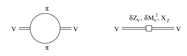
Figure 3: Rho self-energy.

The one loop $\rho$ self-energy contains only an ${\cal O}(p^{4})$ divergence, which renormalizes the coupling $X_{Z}$ of the NLO resonance Lagrangian:

$$X_{Z}\,\equiv\,X_{Z}^{r}(\mu)+\delta X_{Z}(\mu)\qquad\quad;\qquad\quad\delta X_{Z}(\mu)\,=\,-\frac{\displaystyle 2\,G_{V}^{2}}{\displaystyle F^{2}}\,\frac{\displaystyle\lambda_{\infty}}{\displaystyle 192\pi^{2}F^{2}}\;.$$ (25)

Thus, the vector mass and wave-function are not renormalized:

$$\delta M_{V}^{2}\,=\,0\qquad\quad;\qquad\quad\delta Z_{V}\,=\,0\,.$$ (26)

The renormalized $\rho$ self-energy then becomes:

$$-i\,\Sigma_{V}^{r}(q)^{\mu\nu,\rho\sigma}\,=\,-{i\over 2}\,\mathcal{A}^{\mu\nu,\rho\sigma}(q)\;\Sigma_{V}^{r}(q^{2})\,,$$ (27)

where the antisymmetric tensor structure $\mathcal{A}^{\mu\nu,\rho\sigma}(q)$ is defined in appendix B and

$$\Sigma_{V}^{\,r}(q^{2})\,=\,-q^{4}\,\left\{2\,X^{r}_{Z}(\mu)\,-\,\frac{\displaystyle 2\,G_{V}^{2}}{\displaystyle F^{2}}\,\frac{\displaystyle 1}{\displaystyle F^{2}}\,\left[{1\over 6}\,\hat{B}_{0}(q^{2}/\mu^{2})+\frac{\displaystyle 1}{\displaystyle 144\pi^{2}}\right]\right\}\,.$$ (28)

3.3 $\langle v^{\mu}\,V^{\rho\sigma}\rangle$ 1PI vertex

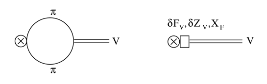
Figure 4: Diagrams contributing to the $\langle v^{\mu}\,V^{\rho\sigma}\rangle$ Green function at NLO in $1/N_{C}$.

The 1PI amputated diagrams (at NLO) connecting an external vector quark current to an outgoing vector resonance are shown in Fig. 4. The one-loop contribution brings an ${\cal O}(p^{4})$ divergence which gets reabsorbed through the following renormalization of the coupling $X_{F}$:

$$X_{F}\,\equiv\,X_{F}^{r}(\mu)+\delta X_{F}(\mu)\qquad\quad;\qquad\quad\delta X_{F}(\mu)\,=\,-\frac{\displaystyle\sqrt{2}\,G_{V}}{\displaystyle F}\,\frac{\displaystyle\lambda_{\infty}}{\displaystyle 192\pi^{2}F}\;.$$ (29)

Since there are no divergences of ${\cal O}(p^{2})$, the lowest-order coupling $F_{V}$ remains unchanged:

$$\delta F_{V}\,=\,0\,.$$ (30)

The renormalized vertex function takes the form

$$i\,\Phi(q)^{\mu,\rho\sigma}\,=\,-i\,\mathcal{I}^{\rho\sigma}_{\alpha\beta}\;q^{\alpha}g^{\mu\beta}\,\left\{F_{V}\,-2\sqrt{2}\,X_{F}^{r}(\mu)\,q^{2}\,+\,\frac{\displaystyle 2G_{V}}{\displaystyle F^{2}}\,q^{2}\,\left[\frac{\displaystyle 1}{\displaystyle 6}\,\hat{B}_{0}(q^{2}/\mu^{2})+\frac{\displaystyle 1}{\displaystyle 144\pi^{2}}\right]\right\}\,,$$ (31)

where the first term is the leading order contribution. The massless two-point function $\hat{B}_{0}(q^{2}/\mu^{2})$ is defined in appendix A and the antisymmetric tensor structure $\mathcal{I}^{\rho\sigma}_{\alpha\beta}$ in appendix B.

3.4 $\langle V_{\mu\nu}\pi\pi\rangle$ 1PI vertex

Figure 5: NLO diagrams contributing to the three-point Green function $V^{\mu\nu}\to\pi\pi$.

The 1PI amputated diagrams connecting a vector resonance with two outgoing pions at NLO in $1/N_{C}$ are shown in Fig. 5. The loop diagrams generate ${\cal O}(p^{2})$ and ${\cal O}(p^{4})$ divergences, which renormalize the couplings $G_{V}$ and $X_{G}$, respectively:

$$G_{V}\,\equiv\,G_{V}^{r}(\mu)+\delta G_{V}(\mu)\qquad;\qquad\delta G_{V}(\mu)\,=\,G_{V}\left[3\,M_{V}^{2}\,\left(\frac{\displaystyle 2G_{V}^{2}}{\displaystyle F^{2}}-\frac{\displaystyle 1}{\displaystyle 2}\right)-M_{S}^{2}\,\frac{\displaystyle 4c_{d}^{2}}{\displaystyle F^{2}}\right]\frac{\displaystyle\lambda_{\infty}}{\displaystyle 16\pi^{2}F^{2}}\;.$$ (32)

$$X_{G}\,\equiv\,X_{G}^{r}(\mu)+\delta X_{G}(\mu)\qquad;\qquad\delta X_{G}(\mu)\,=\,\frac{\displaystyle\sqrt{2}\,G_{V}}{\displaystyle F}\,\left[\frac{\displaystyle 2G_{V}^{2}}{\displaystyle F^{2}}+\frac{\displaystyle 4c_{d}^{2}}{\displaystyle F^{2}}-2\right]\frac{\displaystyle\lambda_{\infty}}{\displaystyle 1536\pi^{2}F}\;.$$ (33)

The wave-function renormalization of the external vector and pion legs amounts to a global factor $\left(\delta Z_{\pi}+\frac{1}{2}\,\delta Z_{V}\right)$ multiplying the lowest-order contribution ($\delta Z_{V}=0$ at NLO). Taking this into account, one finally gets the finite vertex function

$$i\,\Gamma_{\mu\nu}^{\,r}(p_{1},p_{2})\,=\,\mathcal{I}^{\alpha\beta}_{\mu\nu}\;q_{\alpha}(p_{1}-p_{2})_{\beta}\,\frac{\displaystyle 1}{\displaystyle F^{2}}\,\left\{G_{V}^{r}(\mu)\,\left[1-\Delta\Gamma(q^{2},\mu^{2})\right]\,-\,4\sqrt{2}\,X_{G}^{r}(\mu)\,q^{2}\right\}\,,$$ (34)

where

$$\Delta\Gamma(q^{2},\mu^{2}) \!\!= \!\!{1\over F^{2}}\;\left\{\;\hat{B}_{0}(q^{2}/\mu^{2})\;\left[\frac{\displaystyle 2G_{V}^{2}}{\displaystyle F^{2}}\left(\frac{\displaystyle M_{V}^{4}}{\displaystyle q^{2}}+2M_{V}^{2}+\frac{\displaystyle q^{2}}{\displaystyle 12}\right)\,+\,\frac{\displaystyle 4c_{d}^{2}}{\displaystyle F^{2}}\left(\frac{\displaystyle M_{S}^{4}}{\displaystyle q^{2}}+\frac{\displaystyle q^{2}}{\displaystyle 12}\right)-\frac{\displaystyle q^{2}}{\displaystyle 6}\right]\right.$$ (35)

$$\mbox{}+\,\frac{\displaystyle M_{V}^{2}}{\displaystyle 16\pi^{2}}\,\ln{\frac{\displaystyle M_{V}^{2}}{\displaystyle\mu^{2}}}\,\left[\frac{\displaystyle 2G_{V}^{2}}{\displaystyle F^{2}}\left(\frac{\displaystyle M_{V}^{2}}{\displaystyle q^{2}}+5\right)-\frac{\displaystyle 3}{\displaystyle 2}\right]\;+\;\frac{\displaystyle M_{S}^{2}}{\displaystyle 16\pi^{2}}\,\ln{\frac{\displaystyle M_{S}^{2}}{\displaystyle\mu^{2}}}\;\,\frac{\displaystyle 4c_{d}^{2}}{\displaystyle F^{2}}\left(\frac{\displaystyle M_{S}^{2}}{\displaystyle q^{2}}-1\right)$$

$$\mbox{}+\,\frac{\displaystyle M_{V}^{2}}{\displaystyle 64\pi^{2}}\left[3\,\frac{\displaystyle 2G_{V}^{2}}{\displaystyle F^{2}}-1\right]\;+\;\frac{\displaystyle 3M_{S}^{2}}{\displaystyle 64\pi^{2}}\,\frac{\displaystyle 4c_{d}^{2}}{\displaystyle F^{2}}\;+\;\frac{\displaystyle q^{2}}{\displaystyle 288\pi^{2}}\left[\frac{\displaystyle 2G_{V}^{2}}{\displaystyle F^{2}}+\frac{\displaystyle 4c_{d}^{2}}{\displaystyle F^{2}}-2\right]$$

$$\mbox{}+\,\frac{\displaystyle 2G_{V}^{2}}{\displaystyle F^{2}}\;C_{0}(q^{2},0,0,M_{V}^{2})\;\left[\frac{\displaystyle M_{V}^{6}}{\displaystyle q^{2}}+\frac{\displaystyle 5M_{V}^{4}}{\displaystyle 2}+q^{2}M_{V}^{2}\right]$$

$$\mbox{}\left.+\,\frac{\displaystyle 4c_{d}^{2}}{\displaystyle F^{2}}\;C_{0}(q^{2},0,0,M_{S}^{2})\;\left[\frac{\displaystyle M_{S}^{6}}{\displaystyle q^{2}}+\frac{\displaystyle M_{S}^{4}}{\displaystyle 2}\right]\;\right\}\,.$$

The three-propagator integral $C_{0}(q^{2},M_{a}^{2},M_{b}^{2},M_{c}^{2})$ is defined in appendix A.

3.5 $\langle v_{\mu}\pi\pi\rangle$ 1PI vertex

The divergences generated by the 1PI loop diagrams shown in Fig. 6 get reabsorbed through the renormalization of the pion wave function $\delta Z_{\pi}$ and the ${\cal O}(p^{4})$ and ${\cal O}(p^{6})$ couplings $\widetilde{\ell}_{6}$ and $\widetilde{r}^{\phantom{\,r}}_{V2}$:

$$\widetilde{\ell}_{6}\,\equiv\,\widetilde{\ell}^{r}_{6}(\mu)+\delta\widetilde{\ell}_{6}(\mu)\qquad \qquad\delta\widetilde{\ell}_{6}(\mu)\,=\,\left\{3-2\,\frac{\displaystyle 2G_{V}^{2}}{\displaystyle F^{2}}+\frac{\displaystyle 4c_{d}^{2}}{\displaystyle F^{2}}\right\}\,\frac{\displaystyle\lambda_{\infty}}{\displaystyle 96\pi^{2}}\;,$$ ; (36)

$$\widetilde{r}^{\phantom{\,r}}_{V2}\,\equiv\,\widetilde{r}^{\,r}_{V2}(\mu)+\delta\widetilde{r}^{\phantom{\,r}}_{V2}(\mu)\qquad \qquad\delta\widetilde{r}^{\phantom{\,r}}_{V2}(\mu)\,=\,\frac{\displaystyle F^{2}\lambda_{\infty}}{\displaystyle 96\pi^{2}}\,\left\{\frac{\displaystyle 1}{\displaystyle M_{V}^{2}}+\frac{\displaystyle 1}{\displaystyle M_{A}^{2}}\right\}\,.$$ ; (37)

Figure 6: 1PI diagrams connecting an external vector current and two outgoing pions.

The resulting finite correction to the lowest-order pion form factor,

$$\Delta\mathcal{F}(q^{2})_{\mathrm{1PI}}\,=\,\Delta\mathcal{F}^{\,\mathrm{ct}}_{\chi}\,+\,\Delta\mathcal{F}^{\mathcal{L}_{2}}_{\chi}\,+\,\Delta\mathcal{F}^{V}_{\chi}\,+\,\Delta\mathcal{F}^{A}_{\chi}\,+\,\Delta\mathcal{F}^{S}_{\chi}\,+\,\Delta\mathcal{F}^{P}_{\chi}\,,$$ (38)

contains contributions from tree-level counterterms,

$$\Delta\mathcal{F}^{\,\mathrm{ct}}_{\chi} = -\,\frac{\displaystyle 2G_{V}^{2}}{\displaystyle F^{2}}\,\frac{\displaystyle M_{V}^{2}}{\displaystyle 16\pi^{2}F^{2}}\left\{3\,\ln{\frac{\displaystyle M_{V}^{2}}{\displaystyle\mu^{2}}}+\frac{\displaystyle 1}{\displaystyle 2}\right\}\,+\,\frac{\displaystyle 4c_{d}^{2}}{\displaystyle F^{2}}\,\frac{\displaystyle M_{S}^{2}}{\displaystyle 16\pi^{2}F^{2}}\left\{\ln{\frac{\displaystyle M_{S}^{2}}{\displaystyle\mu^{2}}}-\frac{\displaystyle 1}{\displaystyle 2}\right\}$$ (39)

$$\mbox{}-\,\widetilde{\ell}^{r}_{6}(\mu)\,\frac{\displaystyle q^{2}}{\displaystyle F^{2}}\,+\,\widetilde{r}^{\,r}_{V2}(\mu)\,\frac{\displaystyle q^{4}}{\displaystyle F^{4}}\,,$$

and loop diagrams with internal Goldstone bosons (first diagram in Fig. 6),

$$\Delta\mathcal{F}^{\mathcal{L}_{2}}_{\chi}\,=\,\frac{\displaystyle q^{2}}{\displaystyle F^{2}}\left\{\frac{\displaystyle 1}{\displaystyle 6}\,\hat{B}_{0}(q^{2}/\mu^{2})+\frac{\displaystyle 1}{\displaystyle 144\pi^{2}}\right\}\,,$$ (40)

and vector,

$$\Delta\mathcal{F}^{V}_{\chi} = \frac{\displaystyle 2G_{V}^{2}}{\displaystyle F^{2}}\,\frac{\displaystyle 1}{\displaystyle F^{2}}\left\{-\,C_{0}(q^{2},0,0,M_{V}^{2})\,\left[\frac{\displaystyle M_{V}^{6}}{\displaystyle q^{2}}+\frac{\displaystyle 5M_{V}^{4}}{\displaystyle 2}+q^{2}M_{V}^{2}\right]\right.$$

$$\left.\hskip 42.67912pt\mbox{}+\,C_{0}(q^{2},M_{V}^{2},M_{V}^{2},0)\,\left[\frac{\displaystyle M_{V}^{6}}{\displaystyle q^{2}}+\frac{\displaystyle M_{V}^{4}}{\displaystyle 2}\right]\,-\,\hat{B}_{0}(q^{2}/\mu^{2})\,\left[\frac{\displaystyle M_{V}^{4}}{\displaystyle q^{2}}+2M_{V}^{2}+\frac{\displaystyle q^{2}}{\displaystyle 12}\right]\right\}$$

$$\mbox{}-\,\frac{\displaystyle\overline{B}_{0}(q^{2},M_{V}^{2})}{\displaystyle F^{2}}\,\left[\left(2M_{V}^{2}+\frac{\displaystyle q^{2}}{\displaystyle 6}-\frac{\displaystyle q^{4}}{\displaystyle 6M_{V}^{2}}\right)\,+\,\frac{\displaystyle 2G_{V}^{2}}{\displaystyle F^{2}}\left(\frac{\displaystyle M_{V}^{4}}{\displaystyle q^{2}}+\frac{\displaystyle 2M_{V}^{2}}{\displaystyle 3}-\frac{\displaystyle 5q^{2}}{\displaystyle 12}\right)\right]$$

$$\mbox{}+\,\frac{\displaystyle M_{V}^{2}}{\displaystyle 16\pi^{2}F^{2}}\,\ln{\frac{\displaystyle M_{V}^{2}}{\displaystyle\mu^{2}}}\,\left[\left(\frac{\displaystyle q^{2}}{\displaystyle 2M_{V}^{2}}-\frac{\displaystyle q^{4}}{\displaystyle 6M_{V}^{4}}\right)\,-\,\frac{\displaystyle 2G_{V}^{2}}{\displaystyle F^{2}}\left(\frac{\displaystyle M_{V}^{2}}{\displaystyle q^{2}}-1+\frac{\displaystyle 5q^{2}}{\displaystyle 12M_{V}^{2}}\right)\right]$$

$$\mbox{}+\,\frac{\displaystyle M_{V}^{2}}{\displaystyle 16\pi^{2}F^{2}}\left[\left(\frac{\displaystyle q^{2}}{\displaystyle 2M_{V}^{2}}\,-\,\frac{\displaystyle 2q^{4}}{\displaystyle 9M_{V}^{4}}\right)\,+\,\frac{\displaystyle 2G_{V}^{2}}{\displaystyle F^{2}}\left(\frac{\displaystyle M_{V}^{2}}{\displaystyle q^{2}}\,+\,1\,-\,\frac{\displaystyle 19q^{2}}{\displaystyle 36M_{V}^{2}}\right)\right]\,,$$

axial-vector,

$$\Delta\mathcal{F}^{A}_{\chi} = \mbox{}-\,\frac{\displaystyle\overline{B}_{0}(q^{2},M_{A}^{2})}{\displaystyle F^{2}}\left[2M_{A}^{2}+\frac{\displaystyle q^{2}}{\displaystyle 6}-\frac{\displaystyle q^{4}}{\displaystyle 6M_{A}^{2}}\right]\,+\,\frac{\displaystyle M_{A}^{2}}{\displaystyle 16\pi^{2}F^{2}}\ln{\frac{\displaystyle M_{A}^{2}}{\displaystyle\mu^{2}}}\,\left[\frac{\displaystyle q^{2}}{\displaystyle 2M_{A}^{2}}-\frac{\displaystyle q^{4}}{\displaystyle 6M_{A}^{4}}\right]$$ (42)

$$\mbox{}+\,\frac{\displaystyle q^{2}}{\displaystyle 32\pi^{2}F^{2}}\,-\,\frac{\displaystyle q^{4}}{\displaystyle 72\pi^{2}F^{2}M_{A}^{2}}\,,$$

scalar,

$$\Delta\mathcal{F}^{S}_{\chi} = \mbox{}\frac{\displaystyle 4c_{d}^{2}}{\displaystyle F^{2}}\,\frac{\displaystyle 1}{\displaystyle F^{2}}\left\{-\,C_{0}(q^{2},0,0,M_{S}^{2})\,\left[\frac{\displaystyle M_{S}^{6}}{\displaystyle q^{2}}+\frac{\displaystyle M_{S}^{4}}{\displaystyle 2}\right]\,+\,C_{0}(q^{2},M_{S}^{2},M_{S}^{2},0)\,\left[\frac{\displaystyle M_{S}^{6}}{\displaystyle q^{2}}-\frac{\displaystyle M_{S}^{4}}{\displaystyle 2}\right]\right.$$

$$\hskip 42.67912pt\left.\,-\,\hat{B}_{0}(q^{2}/\mu^{2})\,\left[\frac{\displaystyle M_{S}^{4}}{\displaystyle q^{2}}+\frac{\displaystyle q^{2}}{\displaystyle 12}\right]\,+\,\frac{\displaystyle M_{S}^{4}}{\displaystyle 16\pi^{2}q^{2}}\right\}\quad\;-\quad\;\frac{\displaystyle q^{2}}{\displaystyle 288\pi^{2}F^{2}}\left[1+\frac{\displaystyle 1}{\displaystyle 2}\,\frac{\displaystyle 4c_{d}^{2}}{\displaystyle F^{2}}\right]$$

$$\mbox{}-\,\frac{\displaystyle\overline{B}_{0}(q^{2},M_{S}^{2})}{\displaystyle F^{2}}\,\left[\left(\frac{\displaystyle 2M_{S}^{2}}{\displaystyle 3}-\frac{\displaystyle q^{2}}{\displaystyle 6}\right)\,+\,\frac{\displaystyle 4c_{d}^{2}}{\displaystyle F^{2}}\,\left(\frac{\displaystyle M_{S}^{4}}{\displaystyle q^{2}}-\frac{\displaystyle M_{S}^{2}}{\displaystyle 3}+\frac{\displaystyle q^{2}}{\displaystyle 12}\right)\right]$$

$$\mbox{}-\,\frac{\displaystyle M_{S}^{2}}{\displaystyle 16\pi^{2}F^{2}}\,\ln{\frac{\displaystyle M_{S}^{2}}{\displaystyle\mu^{2}}}\,\left[\frac{\displaystyle 4c_{d}^{2}}{\displaystyle F^{2}}\,\left(1+\frac{\displaystyle M_{S}^{2}}{\displaystyle q^{2}}-\frac{\displaystyle q^{2}}{\displaystyle 12M_{S}^{2}}\right)\,+\,\frac{\displaystyle q^{2}}{\displaystyle 6M_{S}^{2}}\right]\,,$$

and pseudoscalar resonances,

$$\Delta\mathcal{F}^{P}_{\chi}\,=\,\frac{\displaystyle\overline{B}_{0}(q^{2},M_{P}^{2})}{\displaystyle F^{2}}\left[-\frac{\displaystyle 2M_{P}^{2}}{\displaystyle 3}+\frac{\displaystyle q^{2}}{\displaystyle 6}\right]\,-\,\frac{\displaystyle q^{2}}{\displaystyle 96\pi^{2}F^{2}}\left[\ln{\frac{\displaystyle M_{P}^{2}}{\displaystyle\mu^{2}}}+\frac{\displaystyle 1}{\displaystyle 3}\right]\,.$$ (44)

4 Vector Form Factor

                   

Figure 7: Basic topologies contributing to the Vector Form Factor at NLO.

The basic topologies contributing to the VFF are shown in Fig. 7, in terms of the NLO 1PI diagrams computed in the previous section. The internal $\rho$ line denotes the dressed vector propagator, including the self-energy correction (28) which regulates the $\rho$ pole. Taking this self-energy into account, the LO contribution takes the form:

$$\mathcal{F}(q^{2})_{\mathrm{LO}}\,=\,1\,+\,\frac{\displaystyle F_{V}\,G_{V}^{\,r}(\mu)}{\displaystyle F^{2}}\;\frac{\displaystyle q^{2}}{\displaystyle M_{V}^{2}-q^{2}-\Sigma^{\,r}_{V}(q^{2})}\;.$$ (45)

The topology in Fig. 7.a generates the following NLO correction:

$$\Delta\mathcal{F}(q^{2})_{F}\,=\,\frac{\displaystyle q^{2}}{\displaystyle M_{V}^{2}-q^{2}-\Sigma^{\,r}_{V}(q^{2})}\;\frac{\displaystyle q^{2}}{\displaystyle F^{2}}\;\left\{\frac{\displaystyle 2G_{V}^{2}}{\displaystyle F^{2}}\,\left[\frac{\displaystyle 1}{\displaystyle 6}\,\hat{B}_{0}(q^{2}/\mu^{2})+\frac{\displaystyle 1}{\displaystyle 144\pi^{2}}\right]-2\,F\,{\sqrt{2}G_{V}\over F}\,X_{F}^{r}(\mu)\right\}\,.$$ (46)

The second topology (Fig. 7.b) brings the contribution:

$$\Delta\mathcal{F}(q^{2})_{G}\,=\,-\,\frac{\displaystyle q^{2}}{\displaystyle M_{V}^{2}-q^{2}-\Sigma^{\,r}_{V}(q^{2})}\;\frac{\displaystyle F_{V}}{\displaystyle\sqrt{2}F}\;\left\{\frac{\displaystyle\sqrt{2}G_{V}}{\displaystyle F}\;\Delta\Gamma(q^{2},\mu^{2})\,+\,\frac{\displaystyle 8\,X_{G}^{r}(\mu)}{\displaystyle F}\,q^{2}\right\}\,,$$ (47)

where $\Delta\Gamma(q^{2},\mu^{2})$ is given in Eq. (35). Finally, Fig. 7.c denotes the 1PI correction $\Delta\mathcal{F}(q^{2})_{\mathrm{1PI}}$ in Eq. (38). Adding all contributions together, one gets the VFF at NLO:

$$\mathcal{F}(q^{2})\,=\,\mathcal{F}(q^{2})_{\mathrm{LO}}\,+\,\Delta\mathcal{F}(q^{2})_{F}\,+\,\Delta\mathcal{F}(q^{2})_{G}\,+\,\Delta\mathcal{F}(q^{2})_{\mathrm{1PI}}\,.$$ (48)

Using the large–$N_{C}$ relations (6) in the NLO terms, the result can be written in the form:

$$\mathcal{F}(q^{2})\;=\;A(q^{2})\;\,{M_{V}^{2}\over M_{V}^{2}-q^{2}-\Sigma^{\,r}_{V}(q^{2})}\;+\;B(q^{2})\,,$$ (49)

where

$$A(q^{2}) = 1+\hat{\delta}_{V}+2\,M_{V}^{2}\,\hat{X}-\Delta\tilde{\Gamma}(q^{2})\,,$$

$$B(q^{2}) = \mathcal{G}(q^{2})-\hat{\delta}_{V}-2\,(M_{V}^{2}+q^{2})\,\hat{X}\,.$$ (50)

The constants

$$\hat{\delta}_{V} \equiv {F_{V}\,G_{V}^{r}(\,\mu)\over F^{2}}-1-\Delta\Gamma(0,\mu^{2})\,,$$

$$\hat{X} \equiv X_{Z}^{r}(\mu)-{1\over F}\,\left[X_{F}^{r}(\mu)+4\,X_{G}^{r}(\mu)\right]$$ (51)

and the functions $\Sigma^{\,r}_{V}(q^{2})$,

$$\Delta\tilde{\Gamma}(q^{2})\;\equiv\;\Delta\Gamma(q^{2},\mu^{2})\,-\,\Delta\Gamma(0,\mu^{2})\,,$$ (52)

and

$$\mathcal{G}(q^{2})\;\equiv\;\Delta\mathcal{F}(q^{2})_{\mathrm{1PI}}\,+\,\Delta\tilde{\Gamma}(q^{2})\;\equiv\;G(q^{2},\mu^{2})\,-\,\Delta\Gamma(0,\mu^{2})$$ (53)

are independent of the renormalization scale $\mu$. The subleading R$\chi$T couplings $X_{F}^{r}(\mu)$ and $X_{G}^{r}(\mu)$ only appear through the constant $\hat{X}$, while $X_{Z}^{r}(\mu)$ is also present in the function $\Sigma^{\,r}_{V}(q^{2})$. At $q^{2}=0$, $\Delta\tilde{\Gamma}(0)=\mathcal{G}(0)=\Sigma^{\,r}_{V}(0)=0$. Therefore $\mathcal{F}(0)=1$ as it should.

Some 1PI diagrams (Figs. 6.a and 6.e and the V terms in Figs. 6.b and 6.c) have a corresponding reducible counterpart involving a vector propagator. The combination of both contributions can be then incorporated in $A(q^{2})$. The function $G(q^{2},\mu^{2})$ contains the corrections generated by the other 1PI diagrams (Figs. 6.d, 6.f, the S term in Fig. 6.b, the S, A and P terms in Fig. 6.c and the $\widetilde{\ell}_{6}$ and $\widetilde{r}^{\phantom{\,r}}_{V2}$ pieces in Fig. 6.g). Subtracting their contribution at $q^{2}=0$, which contains the dependence on the renormalization scale $\mu$,

$$G(0,\mu^{2})\;=\;\Delta\Gamma(0,\mu^{2})\;=\;\frac{\displaystyle 1}{\displaystyle 16\pi^{2}F^{2}}\,\left\{M_{V}^{2}\,\left[\frac{\displaystyle 3}{\displaystyle 2}\,\ln{\frac{\displaystyle M_{V}^{2}}{\displaystyle\mu^{2}}}+\frac{\displaystyle 1}{\displaystyle 4}\right]\,+\,M_{S}^{2}\,\left[-\ln{\frac{\displaystyle M_{S}^{2}}{\displaystyle\mu^{2}}}+\frac{\displaystyle 1}{\displaystyle 2}\right]\right\}\,,$$ (54)

one gets:

$$\mathcal{G}(q^{2}) = \frac{\displaystyle C_{0}(q^{2},M_{V}^{2},M_{V}^{2},0)}{\displaystyle F^{2}}\left[\frac{\displaystyle M_{V}^{6}}{\displaystyle q^{2}}+\frac{\displaystyle M_{V}^{4}}{\displaystyle 2}\right]\;+\;\frac{\displaystyle C_{0}(q^{2},M_{S}^{2},M_{S}^{2},0)}{\displaystyle F^{2}}\left[\frac{\displaystyle M_{S}^{6}}{\displaystyle q^{2}}-\frac{\displaystyle M_{S}^{4}}{\displaystyle 2}\right]$$

$$+\;\frac{\displaystyle\overline{B}_{0}(q^{2},M_{V}^{2})}{\displaystyle F^{2}}\left[-\frac{\displaystyle M_{V}^{4}}{\displaystyle q^{2}}-\frac{\displaystyle 8M_{V}^{2}}{\displaystyle 3}+\frac{\displaystyle q^{2}}{\displaystyle 4}+\frac{\displaystyle q^{4}}{\displaystyle 6M_{V}^{2}}\right]\;+\;\frac{\displaystyle\overline{B}_{0}(q^{2},M_{S}^{2})}{\displaystyle F^{2}}\left[-\frac{\displaystyle M_{S}^{4}}{\displaystyle q^{2}}-\frac{\displaystyle M_{S}^{2}}{\displaystyle 3}+\frac{\displaystyle q^{2}}{\displaystyle 12}\right]$$

$$+\;\frac{\displaystyle\overline{B}_{0}(q^{2},M_{A}^{2})}{\displaystyle F^{2}}\left[-2M_{A}^{2}-\frac{\displaystyle q^{2}}{\displaystyle 6}+\frac{\displaystyle q^{4}}{\displaystyle 6M_{A}^{2}}\right]\;+\;\frac{\displaystyle\overline{B}_{0}(q^{2},M_{P}^{2})}{\displaystyle F^{2}}\left[-\frac{\displaystyle 2M_{P}^{2}}{\displaystyle 3}+\frac{\displaystyle q^{2}}{\displaystyle 6}\right]$$

$$+\;\frac{\displaystyle 1}{\displaystyle 16\pi^{2}F^{2}}\;\left\{\;\frac{\displaystyle M_{V}^{4}+M_{S}^{4}}{\displaystyle q^{2}}\,+\,\frac{\displaystyle 3}{\displaystyle 4}M_{V}^{2}\,-\,\frac{\displaystyle 1}{\displaystyle 4}M_{S}^{2}\right.$$

$$\hskip 42.67912pt+\,q^{2}\,\left[\frac{\displaystyle 1}{\displaystyle 12}\,\ln{\frac{\displaystyle M_{V}^{2}}{\displaystyle\mu^{2}}}+\frac{\displaystyle 1}{\displaystyle 2}\,\ln{\frac{\displaystyle M_{A}^{2}}{\displaystyle\mu^{2}}}-\frac{\displaystyle 1}{\displaystyle 12}\,\ln{\frac{\displaystyle M_{S}^{2}}{\displaystyle\mu^{2}}}-\frac{\displaystyle 1}{\displaystyle 6}\,\ln{\frac{\displaystyle M_{P}^{2}}{\displaystyle\mu^{2}}}+\frac{\displaystyle 4}{\displaystyle 9}-16\pi^{2}\,\widetilde{\ell}_{6}^{r}(\mu)\right]$$

$$\hskip 42.67912pt\left.-\,\frac{\displaystyle q^{4}}{\displaystyle 6}\,\left[\frac{\displaystyle 1}{\displaystyle M_{V}^{2}}\,\ln{\frac{\displaystyle M_{V}^{2}}{\displaystyle\mu^{2}}}+\frac{\displaystyle 1}{\displaystyle M_{A}^{2}}\,\ln{\frac{\displaystyle M_{A}^{2}}{\displaystyle\mu^{2}}}+\frac{\displaystyle 4}{\displaystyle 3}\left(\frac{\displaystyle 1}{\displaystyle M_{V}^{2}}+\frac{\displaystyle 1}{\displaystyle M_{A}^{2}}\right)-\frac{\displaystyle 96\pi^{2}}{\displaystyle F^{2}}\,\widetilde{r}^{\,r}_{V2}(\mu)\right]\;\right\}\,.$$

5 Low-Energy Limit

At very low energies, $q^{2}\ll M_{R}^{2}$, the resonance fields can be integrated out from the effective theory. One recovers then [8] the standard $\chi$PT Lagrangian, which leads to the following result for the VFF [35, 36]:

$$\mathcal{F}_{\chi\mathrm{PT}}(q^{2})\,=\,1\,-\,\frac{\displaystyle q^{2}}{\displaystyle F^{2}}\,\left\{\ell_{6}^{\,r}(\mu)\,+\,\frac{\displaystyle 1}{\displaystyle 96\pi^{2}}\,\left[\ln{\left(-\frac{\displaystyle q^{2}}{\displaystyle\mu^{2}}\right)}-\frac{\displaystyle 5}{\displaystyle 3}\right]\right\}$$

$$\mbox{}+\,\frac{\displaystyle q^{4}}{\displaystyle F^{4}}\,\left\{r^{\,r}_{V2}(\mu)\,+\,\frac{\displaystyle 1}{\displaystyle 96\pi^{2}}\,\left[\ln{\left(-\frac{\displaystyle q^{2}}{\displaystyle\mu^{2}}\right)}-\frac{\displaystyle 5}{\displaystyle 3}\right]\,\left(2\ell_{1}^{\,r}-\ell_{2}^{\,r}+\ell_{6}^{\,r}\right)(\mu)\,+\,{\cal O}\left(\frac{\displaystyle 1}{\displaystyle N_{C}^{2}}\right)\right\}\,+\,{\cal O}\left(\frac{\displaystyle q^{6}}{\displaystyle F^{6}}\right).$$

The Taylor expansion in powers of $q^{2}$ of the R$\chi$T prediction (49) reproduces the $\chi$PT formula (5), as it should. The coefficient of the ${\cal O}\left[q^{4}\ln{(-q^{2}/\mu^{2})}\right]$ term satisfies the known large-$N_{C}$ equality [8, 11] $\left(2\ell_{1}-\ell_{2}+\ell_{6}\right)\,=\,F^{2}(1-5M_{S}^{2}/M_{V}^{2})/(2M_{S}^{2})$. The non-logarithmic ${\cal O}(q^{4})$ and ${\cal O}(q^{6})$ terms relate the low-energy chiral couplings $\ell_{6}$ and $r^{\phantom{\,r}}_{V2}$ with their R$\chi$T counterparts $\widetilde{\ell}_{6}$ and $\widetilde{r}^{\phantom{\,r}}_{V2}$:

$$\ell_{6}^{\,r}(\mu) = \mbox{}-\frac{\displaystyle F^{2}}{\displaystyle M_{V}^{2}}\,(1+\hat{\delta}_{V})\,+\,\widetilde{\ell}_{6}^{\,r}(\mu)\,-\,\frac{\displaystyle 1}{\displaystyle 96\pi^{2}}\,\left[\ln{\frac{\displaystyle M_{V}^{2}}{\displaystyle\mu^{2}}}-\ln{\frac{\displaystyle M_{P}^{2}}{\displaystyle\mu^{2}}}+3\,\ln{\frac{\displaystyle M_{A}^{2}}{\displaystyle\mu^{2}}}-\frac{\displaystyle 13}{\displaystyle 6}\right]$$ (57)

$$= \mbox{}-\frac{\displaystyle F_{V}G_{V}^{\,r}(\mu)}{\displaystyle M_{V}^{2}}\,+\,\widetilde{\ell}_{6}^{\,r}(\mu)\,+\,\frac{\displaystyle 1}{\displaystyle 16\pi^{2}}\,\left[\frac{\displaystyle 4}{\displaystyle 3}\,\ln{\frac{\displaystyle M_{V}^{2}}{\displaystyle\mu^{2}}}-\frac{\displaystyle 1}{\displaystyle 2}\,\ln{\frac{\displaystyle M_{A}^{2}}{\displaystyle\mu^{2}}}+\frac{\displaystyle 1}{\displaystyle 6}\,\ln{\frac{\displaystyle M_{P}^{2}}{\displaystyle\mu^{2}}}-\frac{\displaystyle M_{S}^{2}}{\displaystyle M_{V}^{2}}\,\ln{\frac{\displaystyle M_{S}^{2}}{\displaystyle\mu^{2}}}\right.$$

$$\hskip 156.49014pt\left.\mbox{}+\frac{\displaystyle 11}{\displaystyle 18}+\frac{\displaystyle M_{S}^{2}}{\displaystyle 2M_{V}^{2}}\right]\,,$$

$$r^{\,r}_{V2}(\mu) = \frac{\displaystyle F^{2}F_{V}G_{V}^{\,r}(\mu)}{\displaystyle M_{V}^{4}}\,+\,\widetilde{r}^{\,r}_{V2}(\mu)\,+\,\frac{\displaystyle 2F^{4}}{\displaystyle M_{V}^{2}}\,\left[\hat{X}-X_{Z}^{r}(\mu)\right]$$ (58)

$$\mbox{}+\,\frac{\displaystyle F^{2}}{\displaystyle 96\pi^{2}}\,\left\{\left(6\,\frac{\displaystyle M_{S}^{2}}{\displaystyle M_{V}^{4}}+\frac{\displaystyle 1}{\displaystyle 2M_{V}^{2}}-\frac{\displaystyle 1}{\displaystyle 2M_{S}^{2}}\right)\,\ln{\frac{\displaystyle M_{S}^{2}}{\displaystyle\mu^{2}}}-\frac{\displaystyle 9}{\displaystyle M_{V}^{2}}\,\ln{\frac{\displaystyle M_{V}^{2}}{\displaystyle\mu^{2}}}-\frac{\displaystyle 1}{\displaystyle M_{A}^{2}}\,\ln{\frac{\displaystyle M_{A}^{2}}{\displaystyle\mu^{2}}}\right.$$

$$\hskip 49.79231pt\left.\mbox{}-\frac{\displaystyle 167}{\displaystyle 60M_{V}^{2}}-\frac{\displaystyle 17}{\displaystyle 10M_{A}^{2}}-\frac{\displaystyle 3M_{S}^{2}}{\displaystyle M_{V}^{4}}+\frac{\displaystyle 17}{\displaystyle 20M_{S}^{2}}+\frac{\displaystyle 1}{\displaystyle 10M_{P}^{2}}\right\}\,.$$

Notice that the combination of subleading R$\chi$T couplings $\hat{X}$ does not appear at ${\cal O}(p^{4})$. Therefore, the relation (57) adopts the same form in terms of the effective couplings defined in (19), i.e. $\widetilde{\ell}_{6}^{\,\mathrm{eff},r}(\mu)-F_{V}^{\,\mathrm{eff}}\,G_{V}^{\,\mathrm{eff},r}(\mu)/(M_{V}^{2})^{\mathrm{eff},r}(\mu)=\widetilde{\ell}_{6}^{\,r}(\mu)-F_{V}\,G_{V}^{\,r}(\mu)/M_{V}^{2}$. As shown in (58), this is no longer true at ${\cal O}(p^{6})$; nevertheless, the explicit dependence on $\hat{X}-X_{Z}^{r}(\mu)$ present in $r^{\,r}_{V2}(\mu)$ can be reabsorbed into the leading term, through the use of the effective couplings, i.e. $r^{\,r}_{V2}(\mu)=F^{2}F_{V}^{\,\mathrm{eff}}\,G_{V}^{\,\mathrm{eff},r}(\mu)/(M_{V}^{4})^{\mathrm{eff},r}(\mu)+\widetilde{r}^{\,\mathrm{eff},r}_{V2}+\cdots$

Eqs. (57) and (58) contain the well known lowest-order predictions for the two $\chi$PT couplings: $\ell_{6}=-M_{V}^{2}r^{\,r}_{V2}/F^{2}=-F^{2}/M_{V}^{2}$. Moreover, they give their dependence on the renormalization scale at the NLO. The running of the renormalized couplings [$\ell_{6}^{\,r}(\mu),r^{\,r}_{V2}(\mu)]$ and [$\widetilde{\ell}_{6}^{\,r}(\mu),\widetilde{r}^{\,r}_{V2}(\mu)]$ is different, because their corresponding effective theories have a very different particle content.

The $\mu$ dependence of a given coupling “g” can be characterized through the logarithmic derivative

$$\mu\,\frac{\displaystyle dg}{\displaystyle d\mu}\,=\,-\frac{\displaystyle\gamma_{g}}{\displaystyle 16\pi^{2}}\,.$$ (59)

From Eqs. (36) and (37) one gets the running of the R$\chi$T couplings:

$$\gamma_{\,\widetilde{\ell}_{6}}\,=\,\frac{\displaystyle 2}{\displaystyle 3}\qquad\quad,\qquad\quad\gamma_{\,\widetilde{r}^{\phantom{\,r}}_{V2}}\,=\,\frac{\displaystyle F^{2}}{\displaystyle 3}\,\left(\frac{\displaystyle 1}{\displaystyle M_{V}^{2}}+\frac{\displaystyle 1}{\displaystyle M_{A}^{2}}\right)\,=\,\frac{\displaystyle F^{2}}{\displaystyle 2M_{V}^{2}}\,.$$ (60)

Eqs. (57) and (58) give then the dependence on the renormalization scale of the corresponding $\chi$PT couplings:

$$\gamma_{\ell_{6}}\,=\,-\frac{\displaystyle 1}{\displaystyle 3}\qquad\quad,\qquad\quad\gamma_{r^{\phantom{\,r}}_{V2}}\,=\,\frac{\displaystyle F^{2}}{\displaystyle 6}\,\left(\frac{\displaystyle 5}{\displaystyle M_{V}^{2}}-\frac{\displaystyle 1}{\displaystyle M_{S}^{2}}\right)\,.$$ (61)

These values are in perfect agreement with the low-energy results of refs. [4, 5, 36, 39]. The running of the ${\cal O}(p^{6})$ coupling $r^{\phantom{\,r}}_{V2}(\mu)/F^{4}$ receives of course additional 2-loop contributions which are of ${\cal O}(1/N_{C}^{2})$.

The rigorous control of the renormalization scale dependences allows us to investigate the successful resonance saturation approximation [8] at the NLO. The $\chi$PT couplings $\ell_{6}$ and $r^{\phantom{\,r}}_{V2}$ have been phenomenologically extracted from a fit to the VFF data at low momenta. This determines [36] the scale-invariant combination

$$\bar{\ell}_{6}\,\equiv\,\frac{\displaystyle 32\pi^{2}}{\displaystyle\gamma_{\ell_{6}}}\,\ell_{6}^{\,r}(\mu)\,-\,\log{\frac{\displaystyle m_{\pi}^{2}}{\displaystyle\mu^{2}}}\,=\,16.0\pm 0.5\pm 0.7\,,$$ (62)

and

$$r^{\,r}_{V2}(M_{\rho})\,=\,(1.6\pm 0.5)\cdot 10^{-4}\,.$$ (63)

Inserting these numbers in Eqs. (57) and (58), one can estimate the corresponding scale-invariant combinations of NLO couplings in R$\chi$T:

$$\hat{\ell}_{6}\,\equiv\,\widetilde{\ell}_{6}^{\,r}(\mu)-\frac{\displaystyle\gamma_{\,\widetilde{\ell}_{6}}}{\displaystyle 32\pi^{2}}\,\log{\frac{\displaystyle M_{V}^{2}}{\displaystyle\mu^{2}}}-\frac{\displaystyle F^{2}}{\displaystyle M_{V}^{2}}\,\hat{\delta}_{V}\,,$$ (64)

$$\hat{r}^{\phantom{\,r}}_{V2}\,\equiv\,\widetilde{r}^{\,r}_{V2}(\mu)+\frac{\displaystyle F^{4}}{\displaystyle M_{V}^{4}}\,\left(\hat{\delta}_{V}+2M_{V}^{2}\,\left[\hat{X}-X_{Z}^{r}(\mu)\right]\right)-\frac{\displaystyle\gamma_{\,\widetilde{r}^{\phantom{\,r}}_{V2}}-\frac{\displaystyle 2F^{4}}{\displaystyle M_{V}^{2}}\,\gamma_{{}_{X_{Z}}}}{\displaystyle 32\pi^{2}}\,\log{\frac{\displaystyle M_{V}^{2}}{\displaystyle\mu^{2}}}\,,$$ (65)

where $\gamma_{{}_{X_{Z}}}=-1/(6F^{2})$. Taking $F=92.4$ MeV, $M_{V}=770$ MeV and $M_{S}=1$ GeV, one gets $\hat{\ell}_{6}=(-0.2\pm 0.9)\cdot 10^{-3}$ and $\hat{r}^{\phantom{\,r}}_{V2}=(-0.2\pm 0.5)\cdot 10^{-4}$, while a larger value of the scalar resonance mass $M_{S}=1.4$ GeV shifts the ${\cal O}(p^{4})$ coupling to $\hat{l}_{6}=(-0.9\pm 0.9)\cdot 10^{-3}$, without affecting $\hat{r}^{\phantom{\,r}}_{V2}$ at the quoted level of accuracy. These numbers should be compared with the large–$N_{C}$ predictions for the $\chi$PT couplings  $\ell_{6}|_{N_{C}\to\infty}=-F^{2}/M_{V}^{2}=-0.014$  and  $r^{\phantom{\,r}}_{V2}|_{N_{C}\to\infty}=F^{4}/M_{V}^{4}=2.1\cdot 10^{-4}$. Put in a different way, the hypothesis $\hat{\ell}_{6}=\hat{r}^{\phantom{\,r}}_{V2}=0$ generates excellent predictions for $\ell_{6}^{\,r}(\mu)$ and $r^{\,r}_{V2}(\mu)$ at any scale $\mu$.

6 Behaviour at Large Energies

At large momentum transfer, the relevant renormalization scale invariant functions take the forms:

$$\mathcal{G}(q^{2}) \!\!= \!\!\frac{\displaystyle 1}{\displaystyle 16\pi^{2}F^{2}}\,\left\{-\;q^{4}\,\left[\frac{\displaystyle 1}{\displaystyle 6}\,\left(\frac{\displaystyle 1}{\displaystyle M_{V}^{2}}+\frac{\displaystyle 1}{\displaystyle M_{A}^{2}}\right)\,\left(\ln{\frac{\displaystyle-q^{2}}{\displaystyle\mu^{2}}}-\frac{\displaystyle 2}{\displaystyle 3}\right)-\frac{\displaystyle 16\pi^{2}}{\displaystyle F^{2}}\,\widetilde{r}_{V2}^{\,r}(\mu)\right]\right.$$ (66)

$$\hskip 45.52458pt\left.\mbox{}+\,q^{2}\,\left[\frac{\displaystyle 1}{\displaystyle 3}\,\ln{\frac{\displaystyle-q^{2}}{\displaystyle\mu^{2}}}+\frac{\displaystyle 16}{\displaystyle 9}-16\pi^{2}\,\widetilde{\ell}_{6}^{\,r}(\mu)\right]\,+\,{\cal O}\left(1\right)\right\}\,,$$

$$\Delta\tilde{\Gamma}(q^{2})\,=\,\frac{\displaystyle M_{V}^{2}}{\displaystyle 16\pi^{2}F^{2}}\,\left\{\ln{\frac{\displaystyle-q^{2}}{\displaystyle M_{V}^{2}}}\,\left[\ln{\frac{\displaystyle q^{2}}{\displaystyle M_{V}^{2}}}-2\right]-\frac{\displaystyle 1}{\displaystyle 2}\,\ln^{2}{\frac{\displaystyle q^{2}}{\displaystyle M_{V}^{2}}}-\frac{\displaystyle\pi^{2}}{\displaystyle 6}+\frac{\displaystyle 9}{\displaystyle 4}+\frac{\displaystyle M_{S}^{2}}{\displaystyle 4\,M_{V}^{2}}\right\}+{\cal O}\left(\frac{\displaystyle 1}{\displaystyle q^{2}}\right)\,,$$ (67)

$$\Sigma^{\,r}_{V}(q^{2})\,=\,\frac{\displaystyle-q^{4}}{\displaystyle 96\pi^{2}F^{2}}\,\left\{\ln{\frac{\displaystyle-q^{2}}{\displaystyle\mu^{2}}}-\frac{\displaystyle 5}{\displaystyle 3}+192\pi^{2}F^{2}\,X^{r}_{Z}(\mu)\right\}\,.$$ (68)

The $\rho$ propagator makes the $A(q^{2})$ piece of the VFF well behaved when $q^{2}\to\infty$. However, the 1PI contributions generate a wrong behaviour $\mathcal{G}(q^{2})\sim q^{4}\,\ln{(-q^{2}/\mu^{2})}$ in the $B(q^{2})$ term, which cannot be eliminated with a local contribution. The problem originates in the two-resonance cut which has an unphysical growing with momenta. Although our leading R$\chi$T Lagrangian (5) only incorporates couplings linear in the resonance fields, the kinetic resonance Lagrangian (4) introduces some bilinear interactions through the chiral connection included in the covariant derivatives. Their couplings are fixed by chiral symmetry and give rise to the 1PI diagrams in Figs. 6.c, 6.d and 6.f. Obviously, these are not the only interactions bilinear in the resonance fields even at large–$N_{C}$ [17, 18, 40, 41]. Therefore, it is not surprising that our calculation is unable to find the correct behaviour at large energies for those contributions with two intermediate resonances.

The contributions with an internal vector propagator in diagrams 6.b and 6.c give us some hint about which pieces could be missing in our calculation. These two diagrams combine with a reducible contribution of the type 7.b: the 1PI $\langle V_{\mu\nu}\pi\pi\rangle$ vertex in Fig. 5.b. The three contributions contain identical loop functions and their sum generates a global factor $M_{V}^{2}/(M_{V}^{2}-q^{2})$, which suppresses the large–$q^{2}$ behaviour. Thus, these corrections have been included in the term $A(q^{2})$.

It seems natural to conjecture that the remaining 1PI contributions with two-resonance cuts should combine with the corresponding reducible topologies, including $\langle VRR\rangle$ and $\langle v^{\mu}RR\rangle$ vertices, to generate the final propagator suppression:

$$G(q^{2})\quad\longrightarrow\quad\frac{\displaystyle M_{V}^{2}}{\displaystyle M_{V}^{2}-q^{2}-\Sigma^{\,r}_{V}(q^{2})}\;\;G(q^{2})\,.$$ (69)

The needed Lagrangian takes the form

$$\mathcal{L}^{2}_{VRR}\,=\,i\,\lambda^{VSS}\,\langle\,V^{\mu\nu}\,\nabla_{\mu}S\,\nabla_{\nu}S\,\rangle\;+\;i\,\lambda^{VPP}\,\langle\,V^{\mu\nu}\,\nabla_{\mu}P\,\nabla_{\nu}P\,\rangle\;+\;\cdots$$ (70)

Our conjecture fixes the new chiral couplings in the large–$N_{C}$ limit. It would be interesting to analyze the contributions of this Lagrangian to appropriate Green functions, following the work of refs. [16, 17, 18], and check whether the couplings predicted by the corresponding short-distance QCD corrections agree with our naive conjecture. In appendix C, we show two simple examples where the presence of the propagator suppression can be demonstrated in a rather straightforward way.

The behaviour at large energies is also constrained by unitarity requirements. Moreover, the local contributions can be forced to vanish at large $q^{2}$ by taking appropriate values of the R$\chi$T couplings. Probably, this could allow us to determine the scale invariant constants $\hat{\ell}_{6}$ and $\hat{r}^{\phantom{\,r}}_{V2}$. We plan to investigate all these points in forthcoming works.

7 Summary

The one-loop analysis of the VFF has shown a series of interesting features. As expected, loop diagrams with massive resonance states in the internal lines generate ultraviolet divergences, which require additional higher-dimensional counterterms in the R$\chi$T Lagrangian. Since these counterterms give rise to tree-level contributions which grow too fast at large momenta, their corresponding couplings should be zero at leading order in the large–$N_{C}$ expansion. Thus, one can establish a well defined counting in powers of $1/N_{C}$ to organize the calculation.

The formal renormalization is completely straightforward at one loop. One can easily determine the $\mu$ dependence of all relevant renormalized couplings. Moreover, the final result is only sensitive to some combinations of the chiral couplings. In fact, using the lowest-order equations of motion, one can eliminate most of the higher-order couplings. Their effects get then reabsorbed into redefinitions of the lowest-order parameters.

Expanding the result in powers of $q^{2}/M_{R}^{2}$, one recovers the usual $\chi$PT expression at low momenta. This relates the low-energy chiral couplings $\ell_{6}$ and $r^{\phantom{\,r}}_{V2}$ with their corresponding R$\chi$T counterparts $\widetilde{\ell}_{6}$ and $\widetilde{r}^{\phantom{\,r}}_{V2}$. The rigorous control of the renormalization scale dependences has allowed us to investigate the successful resonance saturation approximation at the next-to-leading order in $1/N_{C}$. The assumption $\hat{\ell}_{6}=\hat{r}^{\phantom{\,r}}_{V2}=0$ generates excellent predictions for $\ell_{6}^{\,r}(\mu)$ and $r^{\,r}_{V2}(\mu)$ at any scale $\mu$.

At high energies, we have identified a problematic behaviour which originates in the two-resonance cuts: they generate an unphysical increase of the VFF at large values of momentun transfer. This is not surprising, since there are additional contributions generated by interaction terms with several resonances, which have not been included in the minimal R$\chi$T Lagrangian. These new chiral structures should be taken into account to achieve a physical description of the VFF above the two-resonance thresholds. The short-distance QCD constraints can be used to determine their corresponding couplings.

Our calculation represents a first step towards a systematic procedure to evaluate next-to-leading order contributions in the $1/N_{C}$ counting. More work in this direction is in progress.

8 Acknowledgements

We have benefited from useful discussions with Oscar Catà, Gerhard Ecker, Santi Peris, Ximo Prades and Jorge Portolés. This work has been supported in part by the EU HPRN-CT2002-00311 (EURIDICE), by MCYT (Spain) under grant FPA-2001-3031 and by ERDF funds from the EU Commission.

Appendix A: Feynman Integrals

The calculation involves the following Feynman Integrals:

$$A_{0}(M^{2})\,\equiv\,\int\frac{\displaystyle dk^{d}}{\displaystyle i(2\pi)^{d}}\;\frac{\displaystyle 1}{\displaystyle k^{2}+i\epsilon\,-\,M^{2}}\;=\;-\,\frac{\displaystyle M^{2}}{\displaystyle 16\pi^{2}}\,\left[\lambda_{\infty}\,+\,\ln{\frac{\displaystyle M^{2}}{\displaystyle\mu^{2}}}\right]\,,$$ (A.1)

$$B_{0}(q^{2},M_{a}^{2},M_{b}^{2})\,\equiv\,\int\frac{\displaystyle dk^{d}}{\displaystyle i(2\pi)^{d}}\;\frac{\displaystyle 1}{\displaystyle(k^{2}+i\epsilon\,-\,M_{a}^{2})\,[(q-k)^{2}+i\epsilon\,-\,M_{b}^{2}]}$$

$$\qquad=-\,\frac{\displaystyle 1}{\displaystyle 16\pi^{2}}\,\left[\lambda_{\infty}\,+\,\frac{\displaystyle M_{a}^{2}}{\displaystyle M_{a}^{2}-M_{b}^{2}}\ln{\frac{\displaystyle M_{a}^{2}}{\displaystyle\mu^{2}}}\,-\,\frac{\displaystyle M_{b}^{2}}{\displaystyle M_{a}^{2}-M_{b}^{2}}\ln{\frac{\displaystyle M_{b}^{2}}{\displaystyle\mu^{2}}}\right]\,+\,\bar{J}(q^{2},M_{a}^{2},M_{b}^{2})\,,$$

and the finite function

$$C_{0}(q^{2},M_{a}^{2},M_{b}^{2},M_{c}^{2})\,\equiv$$

$$\qquad=\int\frac{\displaystyle dk^{d}}{\displaystyle i(2\pi)^{d}}\;\frac{\displaystyle 1}{\displaystyle[(p_{1}-k)^{2}+i\epsilon\,-\,M_{a}^{2}]\,[(p_{2}+k)^{2}+i\epsilon\,-\,M_{b}^{2}]\,(k^{2}+i\epsilon\,-\,M_{c}^{2})}\;,$$

with $q=p_{1}+p_{2}$ and, with massless outgoing pions, $p_{1}^{2}=p_{2}^{2}=0$. The divergences are collected in the factor

$$\lambda_{\infty}\,=\,\frac{\displaystyle 2\,\mu^{d-4}}{\displaystyle d-4}\,+\,\gamma_{E}\,-\,\ln 4\pi\,-1\,,$$ (A.4)

being  $\gamma_{E}\simeq 0.5772\ldots$  the Euler constant and $\mu$ the renormalization scale.

The two-propagator integral contains the finite function

$$\bar{J}(q^{2},M_{a}^{2},M_{b}^{2}) = \frac{1}{32\pi^{2}}\left\{2+\left[\frac{M_{a}^{2}-M_{b}^{2}}{q^{2}}-\frac{M_{a}^{2}+M_{b}^{2}}{M_{a}^{2}-M_{b}^{2}}\right]\,\ln\frac{M_{b}^{2}}{M_{a}^{2}}\right.$$

$$\left.-\,\frac{\lambda^{1/2}(q^{2},M_{a}^{2},M_{b}^{2})}{q^{2}}\;\ln{\left(\frac{[q^{2}+\lambda^{1/2}(q^{2},M_{a}^{2},M_{b}^{2})]^{2}-(M_{a}^{2}-M_{b}^{2})^{2}}{[q^{2}-\lambda^{1/2}(q^{2},M_{a}^{2},M_{b}^{2})]^{2}-(M_{a}^{2}-M_{b}^{2})^{2}}\right)}\right\}\,,$$

with  $\lambda(x,y,z)\,\equiv\,x^{2}+y^{2}+z^{2}-2xy-2xz-2yz$ . Some useful particular cases are:

$$B_{0}(q^{2},0,0) = -\,\frac{\displaystyle\lambda_{\infty}}{\displaystyle 16\pi^{2}}\,+\,\hat{B}_{0}(q^{2}/\mu^{2})\,,$$

$$B_{0}(q^{2},M^{2},M^{2}) = -\,\frac{\displaystyle 1}{\displaystyle 16\pi^{2}}\left\{\lambda_{\infty}+\ln{\frac{\displaystyle M^{2}}{\displaystyle\mu^{2}}}+1\right\}\,+\,\overline{B}_{0}(q^{2},M^{2})\,,$$ (A.6)

$$B_{0}(q^{2},0,M^{2}) = -\,\frac{\displaystyle 1}{\displaystyle 16\pi^{2}}\left\{\lambda_{\infty}+\ln{\frac{\displaystyle M^{2}}{\displaystyle\mu^{2}}}\right\}\,+\,\bar{J}(q^{2},0,M^{2})\,,$$

with the finite parts

$$\hat{B}_{0}(q^{2}/\mu^{2}) = \frac{\displaystyle 1}{\displaystyle 16\pi^{2}}\,\left\{1-\ln{\left(-\frac{\displaystyle q^{2}}{\displaystyle\mu^{2}}\right)}\right\}\,,$$

$$\overline{B}_{0}(q^{2},M^{2}) \equiv \bar{J}(q^{2},M^{2},M^{2})\,=\,\frac{\displaystyle 1}{\displaystyle 16\pi^{2}}\left\{2-\sigma_{M}\ln{\left(\frac{\displaystyle\sigma_{M}+1}{\displaystyle\sigma_{M}-1}\right)}\right\}\,,$$ (A.7)

$$\bar{J}(q^{2},0,M^{2}) \equiv \frac{\displaystyle 1}{\displaystyle 16\pi^{2}}\left\{1-\left(1-{M^{2}\over q^{2}}\right)\,\ln{\left(1-{q^{2}\over M^{2}}\right)}\right\}\,,$$

where  $\sigma_{M}=\sqrt{1-4M^{2}/q^{2}}$.

The relevant three-propagator integrals are:

$$C_{0}(q^{2},0,0,M^{2}) = -\,\frac{\displaystyle 1}{\displaystyle 16\pi^{2}q^{2}}\,\left\{\mbox{Li}_{2}\left(1+\frac{\displaystyle q^{2}}{\displaystyle M^{2}}\right)-\,\mbox{Li}_{2}(1)\right\}\,,$$

$$C_{0}(q^{2},M^{2},M^{2},0) = \frac{\displaystyle 1}{\displaystyle 16\pi^{2}q^{2}}\;\ln^{2}{\left({\sigma_{M}-1\over\sigma_{M}+1}\right)}\,,$$ (A.8)

where

$$\mbox{Li}_{2}(y)\,\equiv\,-\,\int_{0}^{1}\,\frac{\displaystyle dx}{\displaystyle x}\;\ln{(1-xy)}\,=\,-\,\displaystyle{\int}_{0}^{y}\,\frac{\displaystyle dx}{\displaystyle x}\;\ln{(1-x)}$$ (A.9)

is the usual dilogarithmic function.

Appendix B: Lorentz Structures in the Vector Propagators

In momentum space, the bare vector-field propagator can be written in the form

$$\langle\,V^{\mu\nu}V^{\rho\sigma}\,\rangle_{0}\,=\,\Delta^{\mu\nu,\rho\sigma}(q)\,=\,\frac{\displaystyle 2i}{\displaystyle M_{V}^{2}-q^{2}}\;\mathcal{A}^{\mu\nu,\rho\sigma}(q)\,+\,\frac{\displaystyle 2i}{\displaystyle M_{V}^{2}}\;\Omega^{\mu\nu,\rho\sigma}(q)\,,$$ (B.1)

with the antisymmetric tensors

$$\mathcal{A}_{\mu\nu,\rho\sigma}(q) \equiv \frac{\displaystyle 1}{\displaystyle 2q^{2}}\,\left[\,g_{\mu\rho}q_{\nu}q_{\sigma}-g_{\rho\nu}q_{\mu}q_{\sigma}-(\rho\leftrightarrow\sigma)\,\right]\,,$$

$$\Omega_{\mu\nu,\rho\sigma}(q) \equiv -\,\frac{\displaystyle 1}{\displaystyle 2q^{2}}\,\left[g_{\mu\rho}q_{\nu}q_{\sigma}-g_{\rho\nu}q_{\mu}q_{\sigma}-q^{2}g_{\mu\rho}g_{\nu\sigma}-(\rho\leftrightarrow\sigma)\,\right]\,,$$ (B.2)

$$\mathcal{I}_{\mu\nu,\rho\sigma} \equiv \frac{\displaystyle 1}{\displaystyle 2}\,\left(g_{\mu\rho}g_{\nu\sigma}-g_{\mu\sigma}g_{\nu\rho}\right)\,,$$

obeying the properties:

$$\begin{array}[]{c}\Omega\cdot\mathcal{A}\,=\,\mathcal{A}\cdot\Omega\,=\,0\quad\;,\quad\;\mathcal{A}\cdot\mathcal{A}\,=\,\mathcal{A}\quad\;,\quad\;\Omega\cdot\Omega\,=\,\Omega\quad\;,\quad\;\mathcal{A}\,+\,\Omega\,=\,\mathcal{I}\,,\\[10.0pt] q^{\mu}\,\Omega_{\mu\nu,\rho\sigma}(q)\;=\;q^{\nu}\,\Omega_{\mu\nu,\rho\sigma}(q)\;=\;q^{\rho}\,\Omega_{\mu\nu,\rho\sigma}(q)\;=\;q^{\sigma}\,\Omega_{\mu\nu,\rho\sigma}(q)\;=\;0\,.\end{array}$$ (B.3)

For any antisymmetric tensor $H_{\mu\nu,ab}$, the operator $\mathcal{I}_{cd,\alpha\beta}$ acts like the identity, i.e.

$$H\cdot\mathcal{I}\,=\,\mathcal{I}\cdot H\,=\,H\,.$$ (B.4)

We can then define the antisymmetric inverse $G^{ab,\rho\sigma}$, which satisfies

$$H_{\mu\nu,ab}\;G^{ab,\rho\sigma}\,=\,G_{\mu\nu,ab}\;H^{ab,\rho\sigma}\,=\,\mathcal{I}_{\mu\nu}^{\rho\sigma}\,.$$ (B.5)

The inverse propagator in momentum space is given by

$${\Delta^{-1}(q)}^{\mu\nu,\rho\sigma} = -\,i\,\frac{\displaystyle\left(M_{V}^{2}-q^{2}\right)}{\displaystyle 2}\;\mathcal{A}^{\mu\nu,\rho\sigma}(q)\,-\,i\,\frac{\displaystyle M_{V}^{2}}{\displaystyle 2}\;\Omega^{\mu\nu,\rho\sigma}(q)$$ (B.6)

$$= i\,\frac{\displaystyle q^{2}}{\displaystyle 2}\;\mathcal{A}^{\mu\nu,\rho\sigma}(q)\,-\,i\,\frac{\displaystyle M_{V}^{2}}{\displaystyle 2}\;\mathcal{I}^{\mu\nu,\rho\sigma}\,.$$

Appendix C: Form Factors with Resonances in the Final State

We present here a few examples of current matrix elements with external resonances. They show that in order to implement a correct short-distance behaviour, one needs to introduce additional interactions with more than one resonance field. Moreover, the new chiral couplings can be easily determined.

C.1  Axial form factor to $\mathbf{S^{0}_{I=0}\,\pi^{-}}$

Let us consider the two-point correlation function of two axial currents $J_{A}^{\mu}=\bar{d}\gamma^{\mu}\gamma_{5}u$, in the chiral limit:

$$\Pi_{AA}^{\mu\nu}(q)\,\equiv\,i\int d^{4}x\;\,\mathrm{e}^{iqx}\;\langle 0|T\left(J_{A}^{\mu}(x)J_{A}^{\nu}(0)^{\dagger}\right)|0\rangle\,=\,\left(-g^{\mu\nu}q^{2}+q^{\mu}q^{\nu}\right)\,\Pi_{AA}(q^{2})\,.$$ (C.1)

The associated spectral function Im $\Pi_{AA}(t)$ is a sum of positive contributions corresponding to the different intermediate states. At large $t$, it behaves as a constant. Therefore, since there is an infinite number of possible states, the absorptive contribution of a given intermediate state should vanish at infinite momentum transfer.

Figure 8: Tree-level contributions to $\mathcal{F}_{S\pi}(q^{2})$.

One can easily check that the minimal R$\chi$T Lagrangian of ref. [8], which only contains interactions linear in the resonance fields, generates an absorptive $S^{0}_{I=0}\pi^{-}$ contribution with the wrong behaviour at large momenta: $\mbox{\rm Im}\Pi_{AA}(t)|_{S\pi}\,\sim\,$ constant. The problem can be easily identified analysing the corresponding form factor, defined through the matrix element

$$\langle\,S^{0}_{I=0}\,\pi^{-}|\bar{d}\gamma_{\mu}\gamma_{5}u|0\,\rangle\,=\,-\,2\,i\,\mathcal{F}_{S\pi}(q^{2})\;\left(g_{\mu\nu}-\frac{\displaystyle q_{\mu}q_{\nu}}{\displaystyle q^{2}}\right)\,p_{\pi}^{\nu}\,,$$ (C.2)

where $q^{\mu}=(p_{\pi}+p_{S})^{\mu}$. The lowest-order calculation with the R$\chi$T Lagrangian (diagrams 8.a and 8.b) gives a constant form factor,

$$\mathcal{F}_{S\pi}(q^{2})\,=\,\frac{\displaystyle 2\,c_{d}}{\displaystyle F}\,,$$ (C.3)

which obviously is not vanishing at infinite momentum transfer.

The correct large energy behaviour can be recovered adding the interaction term [41]

$$\mathcal{L}^{2}_{SA}\,=\,\lambda_{1}^{SA}\,\langle\,\left\{\nabla^{\mu}S,A_{\mu\nu}\right\}u^{\nu}\}\,\rangle\,,$$ (C.4)

which modifies the form factor (diagram 8.c):

$$\mathcal{F}_{S\pi}(q^{2})\,=\,\frac{\displaystyle 2c_{d}}{\displaystyle F}\,-\,\sqrt{2}\,\lambda_{1}^{SA}\,\frac{\displaystyle F_{A}}{\displaystyle F}\,\frac{\displaystyle q^{2}}{\displaystyle M_{A}^{2}-q^{2}}\,.$$ (C.5)

Imposing that the form factor must vanish as $q^{2}\to\infty$, the coupling $\lambda_{1}^{SA}$ is constrained to take the value

$$\lambda_{1}^{SA}\,=\,-\,\frac{\displaystyle\sqrt{2}\,c_{d}}{\displaystyle F_{A}}\,=\,-\,\frac{\displaystyle 1}{\displaystyle\sqrt{2}}\,.$$ (C.6)

The resulting form factor adopts then the usual monopolar form

$$\mathcal{F}_{S\pi}(q^{2})\,=\,\frac{\displaystyle M_{A}^{2}}{\displaystyle M_{A}^{2}-q^{2}}\,.$$ (C.7)

C.2  Vector form factor to $\mathbf{R^{0}_{I=1}\,R^{-}}$  ($\mathbf{R=S,\,P}$)

Figure 9: Tree-level contributions to $\mathcal{F}_{RR}(q^{2})$.

The two-point correlation function of two vector currents has a similar behaviour at short distances. Its spectral function behaves as a constant at large momentum transfer, implying that the form factors associated with each intermediate state should vanish at $q^{2}\to\infty$.

The minimal R$\chi$T Lagrangian generates the matrix elements:

$$\langle\,R^{0}_{I=1}(p_{1})\,R^{-}(p_{2})|\,\bar{d}\gamma^{\mu}u\,|0\,\rangle\,=\,\sqrt{2}\,(p_{2}-p_{1})^{\mu}\,\mathcal{F}_{RR}(q^{2})\,,$$ (C.8)

where $R=S,P$ stands for a scalar or a pseudo-scalar resonance. The corresponding form factors are just constant at lowest order (diagram 9.a):

$$\mathcal{F}_{RR}(q^{2})\,=\,1\,.$$ (C.9)

This constant contribution originates in the chiral connection of the resonance kinetic Lagrangians.

It is possible again to recover the right QCD short distance behaviour by adding the interaction terms

$$\mathcal{L}^{2}_{VRR}\,=\,i\,\lambda^{VRR}\,\langle\,V^{\mu\nu}\,\nabla_{\mu}R\,\nabla_{\nu}R\,\rangle\,,$$ (C.10)

which change the form factors to (diagram 9.b)

$$\mathcal{F}_{RR}(q^{2})\,=\,1\,+\,\frac{\displaystyle F_{V}}{\displaystyle\sqrt{2}}\,\lambda^{VRR}\,\frac{\displaystyle q^{2}}{\displaystyle M_{V}^{2}-q^{2}}\,.$$ (C.11)

Imposing a proper high energy behaviour one gets the constraint

$$\lambda^{VRR}\,=\,\frac{\displaystyle\sqrt{2}}{\displaystyle F_{V}}\,=\,\frac{\displaystyle 1}{\displaystyle F}\,,$$ (C.12)

and a monopolar form for the form factors

$$\mathcal{F}_{RR}(q^{2})\,=\,\frac{\displaystyle M_{V}^{2}}{\displaystyle M_{V}^{2}-q^{2}}\,.$$ (C.13)

References

[1] A. Pich, “Aspects of Quantum Chromodynamics”,
Proc. 1999 ICTP Summer School in Particle Physics
(Trieste, Italy, 21 June - 9 July 1999),
eds. G. Senjanović and A. Yu. Smirnov, ICTP Series in
Theoretical Physics – Vol. 16 (World Scientific, Singapore, 2000) 53 [arXiv:hep-ph/0001118].
[2] A. Pich, “Effective Field Theory”,
Proc. Les Houches Summer School of Theoretical Physics
–Probing the Standard Model of Particle Interactions–
(Les Houches, France, 28 July - 5 Sep 1997),
eds. R. Gupta et al (Elsevier Science B.V., Amsterdam, 1999),
Vol. II, 949 [arXiv:hep-ph/9806303].
[3]
S. Weinberg, Physica96A (1979) 327.
[4]
J. Gasser and H. Leutwyler, Ann. Phys.158 (1984) 142.
[5]
J. Gasser and H. Leutwyler, Nucl. Phys. B 250 (1985) 465.
[6]
G. Ecker, Prog. Part. Nucl. Phys.35 (1995) 1.
[7]
A. Pich, Rep. Prog. Phys.58 (1995) 563.
[8]
G. Ecker, J. Gasser, A. Pich and E. de Rafael,
Nucl. Phys. B 321 (1989) 311.
[9]
G. Ecker, J. Gasser, H. Leutwyler, A. Pich and E. de Rafael,
Phys. Lett. B 223 (1989) 425.
[10]
G. ’t Hooft, Nucl. Phys. B 72 (1974) 461,
75 (1974) 461;
E. Witten, Nucl. Phys. B 160 (1979) 57.
[11]
A. Pich, “Colourless Mesons in a Polychromatic World”,
Proc. Workshop on Phenomenology of Large– QCD
(Tempe, Arizona, 9–11 January 2002),
ed. R.F. Lebed (World Scientific, Singapore 2002) p. 239 [arXiv:hep-ph/0205030].
[12]
A.V. Manohar, “Large QCD”,
Proc. Les Houches Summer School of Theoretical Physics
–Probing the Standard Model of Particle Interactions–
(Les Houches, France, 28 July - 5 Sep 1997),
eds. R. Gupta et al (Elsevier Science B.V., Amsterdam, 1999),
Vol. II, p. 1091 [arXiv:hep-ph/9802419].
[13]
S. Peris, M. Perrottet and E. de Rafael, JHEP9805 (1998) 011.
[14]
M.F. Golterman and S. Peris, Phys. Rev. D 61 (2000) 034018.
[15] M. Knecht and E. de Rafael, Phys. Lett. B 424 (1998) 335;
M. Knecht, S. Peris and E. de Rafael, Phys. Lett. B 443 (1998) 255;
M.F. Golterman, S. Peris, B. Phily and E. de Rafael, JHEP0201 (2002) 024.
[16] M. Knecht and A. Nyffeler, Eur. Phys. J. C 21 (2001) 659.
[17] P.D. Ruiz-Femenía, A. Pich and J. Portolés,
JHEP0307 (2003) 003.
[18]
V. Cirigliano, G. Ecker, M. Eidemüller, A. Pich and J. Portolés,
arXiv:hep-ph/0404004 [Phys. Lett. B in press].
[19]
F. Guerrero and A. Pich, Phys. Lett. B 412 (1997) 382.
[20]
D. Gómez Dumm, A. Pich and J. Portolés,
Phys. Rev. D 62 (2000) 054014.
[21]
J.J. Sanz-Cillero and A. Pich, Eur. Phys. J. C 27 (2003) 587.
[22]
A. Pich and J. Portolés, Phys. Rev. D 63 (2001) 093005.
[23]
M. Jamin, J.A. Oller and A. Pich, Nucl. Phys. B 587 (2000) 331.
[24]
M. Jamin, J.A. Oller and A. Pich, Nucl. Phys. B 622 (2002) 279.
[25] E. Pallante and A. Pich,
Phys. Rev. Lett.84 (2000) 2568;
Nucl. Phys. B 592 (2000) 294;
E. Pallante, A. Pich and I. Scimemi, Nucl. Phys. B 617 (2001) 441.
[26]
T.N. Truong, Phys. Rev. Lett.61 (1988) 2526;
A. Dobado, M.J. Herrero and T.N. Truong, Phys. Lett.B 235 (1990) 134;
A. Gómez Nicola and J.R. Peláez, Phys. Rev. D 65 (2002) 054009;
T. Hannah, Phys. Rev. D 55 (1997) 5613.
[27]
J.A. Oller, E. Oset and J.E. Palomar,
Phys. Rev. D 63 (2001) 114009;
J.A. Oller and E. Oset, Phys. Rev. D 60 (1999) 074023.
[28]
O. Catà and S. Peris, Phys. Rev. D 65 (2002) 056014.
[29]
M. Bando, T. Kugo, S. Uehara, K. Yamawaki and T. Yanagida,
Phys. Rev. Lett.54 (1985) 1215;
M. Bando, T. Kugo and K. Yamawaki, Phys. Rep.164 (1988) 217;
T. Fujiwara, T. Kugo, H. Terao, S. Uehara and K. Yamawaki,
Prog. Theor. Phys.73 (1985) 926.
[30]
M. Harada and K. Yamawaki, Phys. Rep.381 (2003) 1;
Phys. Lett. B 297 (1992) 151.
[31]
J. Bijnens, P. Gosdzinsky and P. Talavera, Phys. Lett. B 429 (1998) 111;
JHEP9801 (1998) 014; Nucl. Phys.B501 (1997) 495;
J. Bijnens and P. Gosdzinsky, Phys. Lett. B 388 (1996) 203.
[32]
C.-K. Chow and S.-J. Rey, Nucl. Phys. B 528 (1998) 303;
M. Booth, G. Chiladze and A.F. Falk, Phys. Rev. D 55 (1997) 3092.
[33] E. Jenkins, A.V. Manohar and M.B. Wise,
Phys. Rev. Lett.75 (1995) 2272.
[34]
A. Pich, J. Portolés, I. Rosell and P. Ruiz-Femenía,
work in progress.
[35]
J. Gasser and H. Leutwyler, Nucl. Phys. B 250 (1985) 517.
[36]
J. Bijnens, G. Colangelo and P. Talavera, JHEP9805 (1998) 014.
[37] J. Bijnens and P. Talavera, JHEP0203 (2002) 046.
[38] S. Weinberg, Phys. Rev. Lett.18 (1967) 507.
[39]
J. Bijnens, G. Colangelo and G. Ecker,
JHEP9902 (1999) 020; Ann. Phys. 280 (2000) 100.
[40]
D. Gómez Dumm, A. Pich, and J. Portolés,
Phys. Rev. D 69 (2004) 073002.
[41]
V. Cirigliano, G. Ecker, M. Eidemüller, R. Kaiser, A. Pich, and J. Portolés,
work in progress.