Nonperturbative versus perturbative effects in generalized parton distributions

Abstract

Generalized parton distributions (GPDs) are studied at the hadronic (nonperturbative) scale within different assumptions based on a relativistic constituent quark model. In particular, by means of a meson-cloud model we investigate the role of nonperturbative antiquark degrees of freedom and the valence quark contribution. A QCD evolution of the obtained GPDs is used to add perturbative effects and to investigate the GPDs’ sensitivity to the nonperturbative ingredients of the calculation at larger (experimental) scale.

I Introduction

Generalized parton distributions (GPDs) are basic ingredients in the description of hard exclusive processes (see ref. diehl and references therein). Not only are they generalizations of the well known parton distributions from inclusive deep inelastic scattering (DIS), but being correlation functions they also incorporate non-trivial behavior of hadrons related to the nonperturbative regime of quantum chromodymanics (QCD). At present, apart from the preliminary studies of lattice QCD negele ; goeckeler , one cannot calculate GPDs from first principles, so one has to resort to models or parametrizations.

In fact, the perturbative approach to QCD is able to connect observables at different resolution scales, but the realization of the complete project (i.e. to fully understand the consequences of the dynamics of quarks and gluons) requires the input of unknown nonperturbative matrix elements to provide absolute values for the observables at any scale. In the present paper we intend to apply a radiative parton model procedure which, starting from a low resolution scale $Q_{0}^{2}$, has been able to reproduce and predict (see, e.g., ref. RPM and references therein) the main features of the experimental deep inelastic structure functions at high momentum transfer. The procedure assumes that there exists a scale where the short range (perturbative) part of the interaction is negligible and, therefore, the glue and sea are suppressed, and a long range (confining) part of the interaction produces a proton composed by (three) valence quarks, mainly PaPe . Jaffe and Ross JaRo proposed to ascribe the quark model calculations of matrix elements to that hadronic scale $Q_{0}^{2}$. In this way, quark models summarizing a great deal of hadronic properties may substitute for low-energy parametrizations, while evolution to larger $Q^{2}$ is dictated by perturbative QCD.

In the following we study the nucleon’s GPDs within specific hadron models and address the problem of evolving the input distributions to the experimental scale investigating the effects of different dynamical assumptions. In particular, we want to investigate both the quark core structure of the nucleon and its chiral properties. In fact, the new aspects of the GPDs with respect to the better known parton distributions are related to the socalled ERBL region where the presence of dynamical $q\bar{q}$ pairs, both in the nonperturbative and perturbative regimes, plays a crucial role.

The importance of the chiral structure of nucleons is well established both experimentally and theoretically. The pion cloud associated with chiral symmetry breaking was first discussed in the DIS context by Feynman FeyPHI and Sullivan Sull72 . It leads to flavor symmetry violations in the sea-quark distribution of the nucleons Thomas83 , naturally accounting for the excess of $\bar{d}$ (anti)quarks over $\bar{u}$ (anti)quarks as observed experimentally through the violation of the Gottfried sum rule NMC ; NA51 ; E866 ; Hermes . As discussed by Melnitchouk et al. MST99 , the relatively large asymmetry found in these experiments implies the presence of nontrivial dynamics in the proton sea which does not have a perturbative QCD origin. In particular, a quantitative description of the entire region of the quark momentum fraction $x$ covered by the experiments requires a delicate balance between several competing mechanisms. At larger $x$ the dynamics of the pion cloud provides the bulk of the $\bar{d}-\bar{u}$ asymmetry with DIS from the $\pi N$ component of the nucleon wave function, however also the $\pi\Delta$ arises in the light-cone formulation of the meson-cloud model and it is of some importance in DIS too.

Although the nucleon’s nonperturbative antiquark sea cannot be attributed entirely to its virtual meson cloud Koepf , the role of mesons in DIS is of primary importance, and the idea was developed further giving origin to the meson-cloud model (for a review of early work, see refs. STh98 ; Londergan ; Kumano and references therein). The connection between this model and the chiral properties of QCD was established by investigating the nonanalytic behavior of the $\bar{d}-\bar{u}$ distribution ThMS00 (see, however, chen-ji ). The meson-cloud picture is also suggested by QCD in the limit of large numbers of colors $N_{c}$, where it becomes equivalent to an effective theory of mesons, in which baryons appear as solitons, i.e. classical solutions characterized by a mean meson field Witten . A realization of this idea is achieved in the chiral quark-soliton model, where the effective action is derived from the instanton vacuum of QCD, thus providing a microscopic mechanism for the dynamical breaking of chiral symmetry Diakonov . Flavor asymmetry of the antiquark distributions arises in this model of the nucleon as a sub-leading effect in the limit of large $N_{c}$ Dressler .

An alternative approach to investigate the role of $q\bar{q}$-pairs in DIS and to access the ERBL region, is considering the constituent quarks as complex systems ACMP . Such a scheme has been recently developed in relation to a nonrelativistic constituent quark model, both for parton distributions SVT and GPDs SV .

In the present work we will study the possibility of integrating meson-cloud model effects into the evolution of GPDs. To this end we will assume that GPDs can be written in terms of double distributions Rad99 , involving a given profile function and the forward parton distribution derived in some model. At the same time the model proposed by Melnitchouk et al. MST99 will be adapted to show how the knowledge of the meson-cloud effects can be incorporated within a relativistic quark-valence approach to GPDs. The double distribution (DD) model will be briefly recalled in sect. II. Here the input parton distribution is discussed both in terms of the pure valence contribution derived in light-front relativistic quark models (sect. II.1) and in the meson-cloud model (sect. II.2). Matching sea, gluons and valence-parton distributions in QCD evolution of the obtained GPDs is then briefly described in sect. III, and the results are discussed in sect. IV. Some conclusions are drawn in the final section.

II Modeling GPDs with double distributions

In the following we shall concentrate our attention on the chiral even (helicity conserving) distribution $H^{q}(\overline{x},\xi,Q^{2},t)$ for partons of flavor $q$ at the hadronic scale where the models we are going to discuss are assumed to be valid to evaluate the twist-two amplitude. Such amplitude occurs, for example, in deeply virtual Compton scattering where a lepton exchanges a virtual photon of momentum $q^{\mu}$ with a nucleon of momentum $P^{\mu}$, producing a real photon of momentum ${q^{\prime}}^{\mu}$ and a recoil nucleon of momentum ${P^{\prime}}^{\mu}$. Then $Q^{2}=-q^{\mu}q_{\mu}$ is the space-like virtuality that defines the scale of the process. In a symmetric frame of reference where $q^{\mu}$ and the average nucleon momentum $\overline{P}^{\mu}={\textstyle{1\over 2}}(P^{\mu}+{P^{\prime}}^{\mu})$ are collinear along the $z$ axis and in opposite directions, the quark light-cone momentum is $\overline{k}^{+}=\overline{x}\overline{P}^{+}$, the invariant momentum square is $t=\Delta^{2}=({P^{\prime}}^{\mu}-P^{\mu})^{2}$, and the skewedness $\xi$ describes the longitudinal change of the nucleon momentum, $2\xi=-\Delta^{+}/\overline{P}^{+}$.

For sake of simplicity we follow the common notation which explicitly indicates three variables only $(\overline{x},\xi,t)$ instead of four $(\overline{x},\xi,Q^{2},t)$. We shall come back to the definition of $Q^{2}$ when we discuss the values of the hadronic scale $Q_{0}^{2}$ and the QCD evolution of $H^{q}$ in $Q^{2}$.

We also introduce non-singlet (valence) and singlet quark distributions,

$$H^{NS}(\overline{x},\xi,t)\equiv\sum_{q}\left[H^{q}(\overline{x},\xi,t)+H^{q}(-\overline{x},\xi,t)\right]=H^{NS}(-\overline{x},\xi,t),$$ (1)

$$H^{S}(\overline{x},\xi,t)\equiv\sum_{q}\left[H^{q}(\overline{x},\xi,t)-H^{q}(-\overline{x},\xi,t)\right]=-H^{S}(-\overline{x},\xi,t),$$ (2)

respectively. Besides being symmetric or antisymmetric in $\overline{x}$, they are also symmetric under $\xi\to-\xi$ due to the polynomiality property jig .

The analogous GPD for gluons is symmetric in $\overline{x}$, i.e.

$$H^{g}(\overline{x},\xi,t)=H^{g}(-\overline{x},\xi,t),$$ (3)

and reduces to the gluon density $g(x)$ in the forward limit ($\overline{x}\to x$)

$$H^{g}(x,0,0)=x\,g(x),\quad x>0.$$ (4)

There are two distinct regions: the Dokshitzer-Gribov-Lipatov-Altarelli-Parisi (DGLAP) region, $|\overline{x}|>\xi$, and the Efremov-Radyushkin-Brodsky-Lepage (ERBL) region, $|\overline{x}|<\xi$. The naming derives from the fact that the GPD evolution equations in the region $|\overline{x}|>\xi$ ($|\overline{x}|<\xi$) reduce to the familiar DGLAP (ERBL) equations in the limit $\xi=0$ ($\xi=1$).

The singlet and gluon distributions mix under evolution, while the non-singlet distribution does not.

GPDs depend on the invariant momentum transfer $t$. In particular, the first moment in $\overline{x}$ of $H^{q}(\overline{x},\xi,t)$ is independent of $\xi$ and related to the Dirac form factor of the proton. Thus in phenomenological constructions of GPDs it has been found convenient to assume a factorized $t$ dependence determined by some form factors. This simplifies the QCD evolution considerably because in this way the $t$ dependences of quarks and gluons (which mix under evolution) are not modified during evolution.

The $t$-independent part $H^{q}(\overline{x},\xi)\equiv H^{q}(\overline{x},\xi,t=0)$ is parametrized by a two-component form Rad99 :

$$H^{q}(\overline{x},\xi)=H^{q}_{DD}(\overline{x},\xi)+\theta(\xi-|\overline{x}|)\,D^{q}\left(\frac{\overline{x}}{\xi}\right),$$ (5)

where

$$H^{q}_{DD}(\overline{x},\xi)=\int_{-1}^{1}d\beta\int_{-1+|\beta|}^{1-|\beta|}d\alpha\,\delta(\overline{x}-\beta-\alpha\xi)\,F^{q}(\beta,\alpha).$$ (6)

The D-term contribution $D^{q}$ in eq. (5) completes the parametrization of GPDs, restoring the correct polynomiality properties of GPDs jig ; Pol99b . It has a support only for $|\overline{x}|\leq\xi$, so that it is invisible in the forward limit. The D-term contributes to the singlet-quark and gluon distributions and not to the non-singlet distribution. Its effect under evolution is at the level of a few percent FmcD02b , and in the following it will be disregarded in the input GPDs.

According to Radyushkin’s suggestion Rad99 , the DDs entering eq. (6) are written as

$$F^{q}(\beta,\alpha)=h(\beta,\alpha)\,q(\beta),$$ (7)

where $q(\beta)$ is the forward quark distribution (for the flavor $q$), and the profile function $h(\beta,\alpha)$ is parametrized as Rad99 ; Rad01b

$$h(\beta,\alpha)=\frac{\Gamma(2b+2)}{2^{2b+1}\Gamma^{2}(b+1)}\,\frac{\bigl{[}(1-|\beta|)^{2}-\alpha^{2}\bigr{]}^{b}}{(1-|\beta|)^{2b+1}}.$$ (8)

In eq. (8), the parameter $b$ determines the width of the profile function $h(\beta,\alpha)$ and characterizes the strength of the $\xi$ dependence of the GPDs. It is a free parameter for the valence ($b_{val}$) and sea ($b_{sea}$) contributions to GPDs, which can be used in such an approach as fit parameters in the extraction of GPDs from hard electroproduction observables. The favoured choice is $b_{val}=b_{sea}=1.0$, corresponding to maximum skewedness. With a similar assumption adopted for the gluon distribution one defines $b_{gluon}=2$. The limiting case $b\to\infty$ gives $h(\beta,\alpha)\to\delta(\alpha)\,h(\beta)$ and corresponds to the $\xi$-independent ansatz for the GPD, i.e. $H^{q}(\overline{x},\xi)\to H^{q}(x,\xi=0)=q(x)$, as used in refs. Gui98 ; Vdh98 .

In order to explicitly calculate $H^{q}(\overline{x},\xi)$ in eq. (5) knowledge of the parton distribution $q(x)$ is needed. In the two following subsections details are given about the derivation of $q(x)$.

II.1 Parton distributions and light-front relativistic quark models

Following the lines of ref. diehl2 in two recent papers BPT03 ; BPT04 we discussed a method to evaluate GPDs within light-front constituent quark models (CQMs) at the scale dominated by valence (constituent) degrees of freedom. The comparison of these calculations with predictions in the chiral soliton model and the MIT bag model, as well as the consistency with lattice results for the first moments of GPDs showed that all the phenomelogy for large $\bar{x}$ and small $t$ could be studied within the assumed relativistic CQM. As a drawback of such an approach, the calculation was restricted to the region ${\overline{x}}\geq\xi$ and the generation of $q\bar{q}$ contributions could have a perturbative origin only. In contrast, within the DD-based model both ERBL and DGLAP regions of quark GPDs are populated with any input quark distribution $q(x)$ (with or without sea contribution). In this subsection we only consider valence quarks leaving for the next subsection the case including the sea.

According to the approach of refs. BPT03 ; BPT04 the parton distribution in relativistic light-front CQM takes this simple form:

$$q(x,\mu_{0}^{2})=\sum_{j=1}^{3}\delta_{\tau_{j}\tau_{q}}\int\prod_{i=1}^{3}d\vec{k}_{i}\,\delta\left(\sum_{i=1}^{3}\vec{k}_{i}\right)\,\delta\left(x-\frac{k^{+}_{j}}{M_{0}}\right)|\Psi_{\lambda}^{[c]}(\{\vec{k}_{i};\lambda_{i},\tau_{i}\})|^{2},$$ (9)

where $k_{j}^{+}=(k^{0}_{j}+k_{j}^{3})/\sqrt{2}$ is the quark light-cone momentum, and $M_{0}=\sum_{i}\,\sqrt{{\vec{k}}^{2}_{i}+m^{2}_{i}}$ is the free mass for the three-quark system. $\Psi_{\lambda}^{[c]}(\{\vec{k}_{i};\lambda_{i},\tau_{i}\})$ is the canonical wave function of the nucleon in the instant form; under the assumption that only valence quarks are active, it is obtained by solving an eigenvalue equation for the mass operator within relativistic CQMs.

In the following we will discuss results based on the mass operator for the hypercentral CQM FTV99 , i.e.

$$M=\sum_{i=1}^{3}\sqrt{\vec{k}_{i}^{2}+m_{i}^{2}}-\frac{\tau}{y}+\kappa_{l}\,y,$$ (10)

with $\sum_{i}\vec{k}_{i}=0$, and $m_{i}$ being the constituent quark masses, $y=\sqrt{\vec{\rho}^{2}+\vec{\lambda}^{2}}$ is the radius of the hypersphere in six dimensions and $\vec{\rho}$ and $\vec{\lambda}$ are Jacobi coordinates. For a discussion of the model see refs. FTV99 ; GE95 .

The distribution (9) automatically fulfills the support condition and satisfies the (particle) baryon number and momentum sum rules at the hadronic scale $\mu_{0}^{2}$ where the valence contribution dominates the twist-two response:

$$\int dx\,q(x,\mu_{0}^{2})=N_{q},$$ (11)

with $N_{q}$ being the number of valence quarks of flavor $q$,

$$\int dx\,x\,[u(x,\mu_{0}^{2})+d(x,\mu_{0}^{2})]=1,$$ (12)

and $u(x,\mu_{0}^{2})\equiv u_{V}(x,\mu_{0}^{2})$ and $d(x,\mu_{0}^{2})\equiv d_{V}(x,\mu_{0}^{2})$, the up and down valence-quark distributions.

II.2 Parton distributions and the meson-cloud model

Let us now introduce the meson-cloud model to incorporate $q\bar{q}$ contributions into the valence-quark model of the parton distribution discussed in the previous section.

The basic hypothesis of the meson-cloud model is that the physical nucleon state can be expanded (in the infinite momentum frame (IMF) and in the one-meson approximation) in a series involving bare nucleons and two-particle, meson-baryon states. Its wave function is written as the sum of meson-baryon Fock states

$$|p\rangle=\sqrt{Z}|p\rangle_{bare}+\sum_{BM}\int dy\,d^{2}\vec{k}_{\perp}\,\phi_{BM}(y,k_{\perp}^{2})\,|B(y,\vec{k}_{\perp});M(1-y,-\vec{k}_{\perp})\rangle.$$ (13)

Here $\phi_{BM}(y,k_{\perp}^{2})$ is the probability amplitude for the proton to fluctuate into a virtual baryon-meson $BM$ system with the baryon and meson having longitudinal momentum fractions $y$ and $1-y$ and transverse momenta $\vec{k}_{\perp}$ and $-\vec{k}_{\perp}$, respectively. $Z$ is the wave function renormalization constant and is equal to the probability to find the bare proton in the physical proton.

The lowest lying fluctuations for the proton which we include in our calculation are

$$p(uud) \rightarrow n(udd)\,\pi^{+}(u\bar{d}),$$

$$p(uud) \rightarrow p(uud)\,\pi^{0}\left(\frac{1}{\sqrt{2}}[d\bar{d}-u\bar{u}]\right),$$

$$p(uud) \rightarrow \Delta^{+}(uud)\,\pi^{0}\left(\frac{1}{\sqrt{2}}[d\bar{d}-u\bar{u}]\right),$$

$$p(uud) \rightarrow \Delta^{0}(udd)\,\pi^{+}(u\bar{d}),$$

$$p(uud) \rightarrow \Delta^{++}(uuu)\,\pi^{-}(\bar{u}d).$$ (14)

In DIS the virtual photon can hit either the bare proton $p$ or one of the constituents of the higher Fock states. In the IMF, where the constituents of the target can be regarded as free during the interaction time, the contribution of the higher Fock states to the quark distribution of the physical proton, can be written as the convolution

$$\delta q_{p}(x)=\sum_{MB}\left[\int_{x}^{1}\frac{dy}{y}\,f_{MB/p}(y)\,q_{M}\left(\frac{x}{y}\right)+\int_{x}^{1}\frac{dy}{y}\,f_{BM/p}(y)\,q_{B}\left(\frac{x}{y}\right)\right],$$ (15)

where the splitting functions $f_{MB/p}(y)$ and $f_{BM/p}(y)$ are related to the probability amplitudes $\phi_{BM}$ by

$$f_{BM/p}(y)=f_{MB/p}(1-y)=\int_{0}^{\infty}dk_{\perp}^{2}\sum_{\lambda,\lambda^{\prime}}\left|\phi_{BM}^{\lambda\lambda^{\prime}}(y,k_{\perp}^{2})\right|^{2}.$$ (16)

Here $\phi_{BM}^{\lambda\lambda^{\prime}}(y,k_{\perp}^{2})$ is the probability amplitude for a hadron with given positive helicity to be in a Fock state consisting of a baryon with helicity $\lambda$ and a meson with helicity $\lambda^{\prime}$ BoTho99 . It can be calculated by using time-ordered perturbation theory in the IMF. The quark distributions in a physical proton are then given by

$$q_{p}(x)=Zq_{p}^{bare}(x)+\delta q_{p}(x),$$ (17)

where $q_{p}^{bare}$ are the bare quark distributions and the renormalization constant $Z$ is given by

$$Z\equiv 1-\sum_{MB}\int_{0}^{1}dy\,f_{MB/p}(y).$$ (18)

The amplitudes $\phi^{\lambda\lambda^{\prime}}_{BM}(y,k_{\perp}^{2})$ may be expressed in the following form

$$\phi^{\lambda\lambda^{\prime}}_{BM}(y,k_{\perp}^{2})=\frac{1}{2\pi\sqrt{y(1-y)}}\frac{\sqrt{m_{H}m_{B}}}{m^{2}_{H}-{\cal M}_{BM}^{2}(y,k_{\perp}^{2})}\,G_{HBM}(y,k_{\perp}^{2})V^{\lambda\lambda^{\prime}}_{IMF}(y,k_{\perp}^{2}),$$ (19)

where $m_{H}$ is the physical mass of the fluctuating hadron (in present case the proton, but the approach can be generalized (e.g. ref. BoTho99 )), and

$${\cal M}_{BM}^{2}=\frac{k_{\perp}^{2}+m_{B}^{2}}{y}+\frac{k_{\perp}^{2}+m_{M}^{2}}{1-y}$$ (20)

is the invariant mass of the meson-baryon fluctuation. $V^{\lambda\lambda^{\prime}}_{IMF}(y,k_{\perp}^{2})$ describes the vertex and contains the spin-dependence of the amplitude. The exact form of the $V^{\lambda\lambda^{\prime}}_{IMF}(y,k_{\perp}^{2})$ can be found for various transitions in refs. STh98 ; HSS96 . Because of the extended nature of the vertices one has to introduce phenomenological vertex form factors, $G_{HBM}(y,k^{2}_{\perp})$, which parametrize the unknown dynamics at the vertices. We use the popular parametrization

$$G_{HBM}(y,k_{\perp}^{2})=\left(\frac{\Lambda^{2}_{BM}+m_{H}^{2}}{\Lambda^{2}_{BM}+{\cal M}^{2}_{BM}(y,k_{\perp}^{2})}\right)^{2}.$$ (21)

In order to calculate the meson-cloud corrections to the quark distributions we have to specify the coupling constants entering $V^{\lambda\lambda^{\prime}}_{IMF}(y,k_{\perp}^{2})$ and the cut-off parameters $\Lambda_{BM}$. We use the numerical values as given by MST99 ; BoTho99 , i.e. $g^{2}_{NN\pi}/4\pi=13.6$ and $g^{2}_{N\Delta\pi}/4\pi=11.08$ GeV^-2. The couplings of a given type of fluctuation with different isospin components are related by isospin Clebsch-Gordon coefficients, $g_{pn\pi^{+}}=-\sqrt{2}g_{pp\pi^{0}}$, $g_{p\Delta^{0}\pi^{+}}=-g_{p\Delta^{+}\pi^{0}}/\sqrt{2}=g_{p\Delta^{++}\pi^{-}}/\sqrt{3}$, with $g_{NN\pi}=g_{pp\pi^{0}}$ and $g_{N\Delta\pi}=g_{p\Delta^{++}\pi^{-}}$. The violation of the Gottfried sum rule and flavor symmetry puts also constraints on the magnitude of the cut-off parameters. The values $\Lambda_{MB}=1.0$ GeV and $\Lambda_{MB}=1.3$ GeV for the $\pi N$ and $\pi\Delta$ components, respectively, give contributions to the $\bar{u}$ and $\bar{d}$ which are consistent with the requirement that the meson-cloud component of the sea quark contribution cannot be larger than the measured sea quark and also with flavor symmetry violation MST99 . With this choice of the parameters the probabilities of the fluctuations are given by $P_{N\pi/p}=13\%$, $P_{\Delta\pi/p}=11\%$.

In the following we will assume that at the lowest hadronic scale the bare nucleon is described by the relativistic quark model wave function formulated within the light-front dynamics and, as a consequence, that only valence partons will contribute to the partonic content of the bare nucleon FTV99 ; BPT03 . The full (nonperturbative) antiquark content will be generated by the meson-cloud mechanism described by eq. (15). The partonic content of the $\Delta$ and the pion will be consistently evaluated within the same scheme assuming light-front dynamics and valence contributions only. Within these approximations the meson-cloud corrections at the hadronic scale $\mu_{0}^{2}$ read

$$q_{p}(x)=Zq_{p}^{bare}(x) + \int_{x}^{1}\frac{dy}{y}\left[f_{N\pi/p}(1-y)+f_{\Delta\pi/p}(1-y)\right]q_{\pi}\left(\frac{x}{y}\right)$$ (22)

$$+ \int_{x}^{1}\frac{dy}{y}\left[f_{N\pi/p}(y)+f_{\Delta\pi/p}(y)\right]q_{\Delta}\left(\frac{x}{y}\right),$$

where $q_{p}\equiv(u=u_{V}+\bar{u},d=d_{V}+\bar{d})$ include both valence and sea contribution coming from the meson-baryon fluctuations, while $q_{p}^{bare}\equiv(u_{V}^{bare},d_{V}^{bare})$ include the valence contribution only as discussed in section II.1. The conservation of both momentum and baryon number sum rules is guaranteed by the correct formulation of meson-cloud approach, in particular by the momentum conservation due to the symmetry $f_{BM/p}(y)=f_{MB/p}(1-y)$ in eq. (15) and by the renormalization factor $Z$ of eqs. (13), (17) and (18).

The nucleon

In order to model the partonic content at the scale $\mu_{0}^{2}$ for the nucleon, the $\Delta$ and the pion, we make use of the light-front approach discussed in sect. II.1 and calculate the diagonal component of the generalized parton distributions, i.e. the inclusive parton distributions by means of

$$q_{p}^{bare}(x)\equiv q(x,\mu_{0}^{2}),$$ (23)

where $q(x,\mu_{0}^{2})$ is given by eq. (9).

The $\Delta$

The calculation of the cloud contribution involves the explicit form for the parton distributions $q_{\Delta}(x)$ of the $\Delta$ (see eq. (22)); we use the results of the relativistic model for the nucleon and the isospin symmetries:

$$\begin{array}[]{lcllcl}u_{\Delta^{++}}(x,\mu_{0}^{2})&=&\frac{3}{2}u_{p}(x,\mu_{0}^{2}),&d_{\Delta^{++}}(x,\mu_{0}^{2})&=&0,\\ u_{\Delta^{+}}(x,\mu_{0}^{2})&=&u_{p}(x,\mu_{0}^{2}),&d_{\Delta^{+}}(x,\mu_{0}^{2})&=&d_{p}(x,\mu_{0}^{2}),\\ u_{\Delta^{0}}(x,\mu_{0}^{2})&=&\frac{1}{2}u_{p}(x,\mu_{0}^{2}),&d_{\Delta^{0}}(x,\mu_{0}^{2})&=&2\,d_{p}(x,\mu_{0}^{2}),\\ u_{\Delta^{-}}(x,\mu_{0}^{2})&=&0,&d_{\Delta^{-}}(x,\mu_{0}^{2})&=&3\,d_{p}(x,\mu_{0}^{2}).\end{array}$$ (24)

The pion

The canonical wave function of the pion is taken from ref. Choi99 and reads

$$\Psi^{[c]}(\vec{k}_{1},\vec{k}_{2};\mu_{1},\mu_{2})=\frac{1}{\pi^{3/4}\beta^{3/2}}\left({\textstyle{1\over 2}}\mu_{1}{\textstyle{1\over 2}}\mu_{2}|00\right)\exp{(-k^{2}/(2\beta^{2}))},$$ (25)

with $\vec{k}=\vec{k}_{1}=-\vec{k}_{2}$, $x=x_{1}=k^{+}/M_{0},$ $x_{2}=1-x$, $M_{0}^{2}=(\vec{k}_{\perp}^{2}+m_{q}^{2})/x+(\vec{k}_{\perp}^{2}+m_{q}^{2})/(1-x)$, and $\beta=0.3659$ GeV. The choice of the model from ref. Choi99 is consistent with the hypercentral CQM we adopt for the nucleon, in fact the central potential between the two constituent quarks is described as a linear confining term plus Coulomb-like interaction. The canonical expression (25) represents a variational solution to the mass equation.

The light-front parton distribution of the $\pi^{+}$ is given by

$$q_{\pi^{+}}(x)=v_{\pi}(x,\mu_{0}^{2}) = \sum_{j=1}^{2}\delta_{\tau_{j}\tau_{q}}\int\prod_{i=1}^{2}d\vec{k}_{i}\,\delta\left(\sum_{i=1}^{2}\vec{k}_{i}\right)\,\delta\left(x-\frac{k^{+}_{j}}{M_{0}}\right)$$ (26)

$$\qquad\times\left|\Psi_{\lambda}^{[c]}(\{\vec{k}_{i};\lambda_{i}\})\right|^{2}\left|\left({\textstyle{1\over 2}}\tau_{j}{\textstyle{1\over 2}}-\tau_{j}|00\right)\right|^{2}.$$

Isospin symmetry imposes $u_{V}^{\pi^{+}}=\bar{d}_{V}^{\pi^{+}}=\bar{u}_{V}^{\pi^{-}}=d_{V}^{\pi^{-}}=v_{\pi}(x,\mu_{0}^{2})$, while, due to the model restrictions, the pion sea at the hadronic scale vanishes: $\bar{u}^{\pi^{+}}=d^{\pi^{+}}=u^{\pi^{-}}=\bar{d}^{\pi^{-}}=0$.

III Matching sea, gluons and valence-parton distributions in QCD evolution

In order to extract the parton distributions of the nucleon including the sea (cloud) contributions we need to match sea, valence and gluons within the radiative parton model and to identify the matching scale $Q_{0}^{2}$ consistent with QCD evolution equation GRV9295 ; TVMZ97 .

We assume that the gluon distribution has a valence-like form and reads

$$G(x,Q_{0}^{2})=\frac{N_{g}}{3}\left[u_{V}(x,Q_{0}^{2})+d_{V}(x,Q_{0}^{2})\right],$$ (27)

where $N_{g}$ represents the number of gluons. Since $\int dx\left[u_{V}(x,Q_{0}^{2})+d_{V}(x,Q_{0}^{2})\right]=2+1$ because of baryon number conservation, we have

$$\int dx\,G(x,Q_{0}^{2})=\frac{N_{g}}{3}\int dx\left[u_{V}(x,Q_{0}^{2})+d_{V}(x,Q_{0}^{2})\right]=N_{g}.$$ (28)

Following Glück et al. GRV9295 , we fix $N_{g}=2$, the minimum number of gluons one needs to build a color singlet state. In spite of the simplicity of the assumption in eq. (27), the analysis of refs. GRV9295 ; TVMZ97 shows that the crucial ingredient in the formulation of the radiative parton model is the amount of gluon momentum more than its actual form. Of course, to be really predictive one has to fit the form of the gluon distribution in a quite precise way, an accuracy which goes beyond the aim of the present study.

The total momentum carried at the scale $Q_{0}^{2}$ (the scale of the physical proton, which will be larger than the scale of the bare proton $\mu_{0}^{2}$ made up of three valence only) must fulfill the requirement

$$\int dx\,x\left[G(x,Q_{0}^{2})+u_{V}(x,Q_{0}^{2})+d_{V}(x,Q_{0}^{2})+2\,\left[\bar{u}(x,Q_{0}^{2})+\bar{d}(x,Q_{0}^{2})\right]\right]=1,$$ (29)

and consequently

$$\int dx\,x\left[u_{V}(x,Q_{0}^{2})+d_{V}(x,Q_{0}^{2})\right]$$

$$\quad=\frac{1}{1+\frac{N_{g}}{3}}\left[1-\int dx\,2\,x\left[\bar{u}(x,Q_{0}^{2})+\bar{d}(x,Q_{0}^{2})\right]\right]=0.52.$$ (30)

In conclusion, by using the notation $\langle f\rangle_{n}=\int dx\,x^{n-1}f(x)$ for the moments, we have $\langle u_{V}+d_{V}\rangle_{2}=0.52$, $\langle G\rangle_{2}=0.35$, $\langle 2\left(\bar{u}+\bar{d}\right)\rangle_{2}=0.13$, consistent with a next-to-leading order (NLO) evolution of the moments (in the DIS renormalization scheme) with $Q_{0}^{2}=0.27$ GeV² and $\Lambda_{\rm NLO}=0.248$ GeV GRV9295 ; TVMZ97 .

The actual values of $Q_{0}^{2}$ are fixed TVMZ97 evolving back unpolarized data, until the valence distribution matches the required momentum $\langle u_{V}+d_{V}\rangle_{2}=0.52$. The procedure makes use of the valence contribution only, and it does not depend on the renormalization scheme. The value of $\Lambda_{\rm NLO}$ is suggested by the analysis of Glück et al. GRV9295 , the coupling $\left.\alpha_{s}(Q_{0}^{2})\right|_{\rm NLO}$ is obtained evolving back the valence distribution as previously discussed, and $Q_{0}^{2}$ is found by solving numerically the NLO transcendental equation

$$\ln{Q_{0}^{2}\over\Lambda_{\rm NLO}^{2}}-{4\,\pi\over\beta_{0}\,\alpha_{s}}+{\beta_{1}\over\beta_{0}^{2}}\,\ln\left[{4\,\pi\over\beta_{0}\,\alpha_{s}}+{\beta_{1}\over\beta_{0}^{2}}\right]=0\,,$$ (31)

which assumes the more familiar expression

$${\alpha_{s}(Q^{2})\over 4\pi}={1\over\beta_{0}\ln(Q^{2}/\Lambda_{\rm NLO}^{2})}\left(1-{\beta_{0}\over\beta_{0}^{2}}\,{\ln\ln(Q^{2}/\Lambda_{\rm NLO}^{2})\over\ln(Q^{2}/\Lambda_{\rm NLO}^{2})}\right)$$ (32)

only in the limit $Q^{2}\gg\Lambda_{\rm NLO}^{2}$ (an interesting discussion about the effects of the approximation (32) can be found in ref. WM96 ).

The hadronic scale, $\mu_{0}^{2}$, consistent with the presence of valence degrees of freedom only (as discussed in sect. II.1), is much lower and consistent with the constituent quark mass, its actual value being $\mu_{0}^{2}=0.094$ GeV². The NLO evolution of the unpolarized distributions is performed following the solution of the renormalization group equation in terms of moments, i.e. $\langle f(Q^{2})\rangle_{n}=\int_{0}^{1}dx\,f(x,Q^{2})\,x^{n-1}$, and involves kernels which have been computed up to next-to-leading order (NLO) in perturbation theory BeMu . Since, in our case, the starting points for the evolution ($\mu_{0}^{2},Q_{0}^{2}$) are rather low, the form of the equations must guarantee complete symmetry for the evolution from $\mu_{0}^{2}$ to $Q^{2}\gg\mu_{0}^{2}$ and back  avoiding additional approximations associated with Taylor expansions and not with the genuine perturbative QCD expansion TVMZ97 ; WM96 .

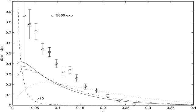
Figure 1: $\bar{d}-\bar{u}$ distribution: at the scale $Q_{0}^{2}=0.27$ (GeV/c)² (dotted curve), at the (average) scale $Q^{2}=54$ (GeV/c)² of the E866 experiment (solid curve), at the comparison scale of $Q^{2}=5$ (GeV/c)² (dot-dashed). The result (multiplied by a factor 10 for convenience) of an evolution starting from the lowest hadronic scale where the nonperturbative sea content is neglected is also shown (dashed). Data from the E866 experiment E866 .

In Fig. 1 we compare our results for the $\bar{d}-\bar{u}$ difference with the data from the E866 experiment E866 . A QCD evolution with an SU(6) symmetric input introduces a very small amount of asymmetric sea at the experimental scale. Within our approach such an assumption corresponds to the perturbative contribution coming from three valence quark distributions at the lowest hadronic scale as predicted by the relativistic model of eq. (9) BPT03 . The presence of the nonperturbative sea introduced by means of the meson-cloud model discussed in the present section improves quite substantially the comparison with the experimental data. In particular let us note: $i$) the important role played also by perturbative evolution in the region $x<0.1$ once the nonperturbative sea and gluon content is introduced at the hadronic scale $Q_{0}^{2}$; $ii$) the satisfactory result in spite of our simple model. All evolutions have been performed according to ref. TVMZ97

IV Results and discussion

Results are presented in this section according to the model based on DDs as described in sect. II. In particular, we will take: $i$) forward parton distributions with only valence quarks (section II.1) at input scale $\mu_{0}^{2}=0.094$ GeV² for the DDs, and $ii$) parton distributions generated including meson-cloud corrections as in eq. (22) and matched with the gluon distribution at an input scale $Q_{0}^{2}=0.27$ GeV², as described in section II.2. In both cases our input GPDs are continuous functions all over the whole range $\overline{x}\in[-1,1]$. The $t$ dependence is dropped from the very beginning and could be reintroduced in the final results by an appropriate $t$-dependent factor. The D-term is omitted as well.

In addition to the results at the hadronic scale we will discuss the evolution of GPDs at higher scale. The QCD evolution was numerically performed to NLO accuracy (in the $\overline{\mbox{MS}}$ scheme), according to a modified version of the code of ref. FmcD02b (see also FmcD02a ; FmcDS03 ). The modifications we introduced in the main code are basically due to the need of a complete NLO evolution which makes use of the correct NLO transcendental equation (31). The original code makes use of the simplified expression (32) largely unsatisfactory for our pourposes.

In fig. 2 results are shown for the singlet quark, non-singlet quark and gluon GPDs obtained with no initial gluons and an input $q(\beta)$ in eq. (7) simply given by the bare (valence) parton distribution $q_{p}^{bare}(x)$, eq. (9), derived from the hypercentral CQM. The model already gives a nonvanishing contribution to quark GPDs in the ERBL region at the hadronic scale $\mu_{0}^{2}$ without introducing discontinuities at $\overline{x}=\xi$ and with a weak $\xi$ dependence. In particular, the absence of the sea contribution gives $H^{S}=H^{NS}$ at $\overline{x}>\xi$. After evolution up to $Q^{2}=5$ GeV² GPDs are almost confined into the ERBL region with a significant $\xi$ dependence.

This behavior is in agreement with previous studies of the GPD evolution showing that as the resolution scale increases the distributions are swept from the DGLAP domain to lie fully within the ERBL region GoMa ; shuvaev . Functions with support entirely in the time-like ERBL region $|\overline{x}|<\xi$ are never pushed out of the ERBL domain. In fact, the evolution in the ERBL region depends on the DGLAP region, whereas the DGLAP evolution is independent of the ERBL region.

The same GPDs obtained when the input is implemented with the sea according to the meson-cloud model, i.e. $q_{p}(x)$ of eq. (22), are shown in fig. 3. Now, the gluon GPD does no more vanish at the initial hadronic scale, that has to be redefined at $Q_{0}^{2}=0.27$ GeV² according to the conclusion of sect. III. After evolution the qualitative result is similar to the case without the sea in spite of a more evident $\xi$ dependence of the singlet quark GPD at the input hadronic scale. However, the shape of the non-singlet quark GPD around $\overline{x}=0$ is sensitive to the input, and the $\xi$ dependence of the GPDs size is in general less pronounced.

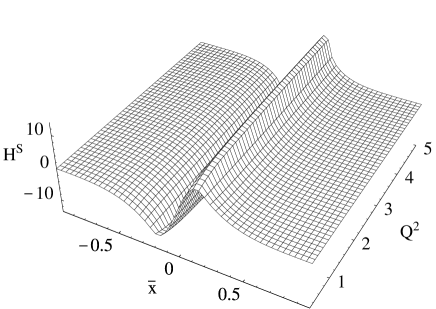
Figure 4: Singlet quark GPD at $\xi=0.2$ as a function of $\overline{x}$ and $Q^{2}$ obtained from NLO evolution of the GPDs using input parton distributions of the hypercentral CQM with the sea contribution at the initial scale $Q_{0}^{2}$.

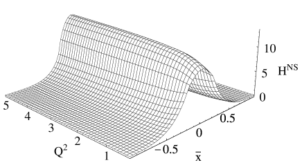
Figure 5: Same as in fig. 4, but for the non-singlet quark GPD.

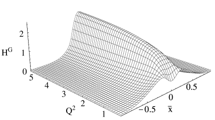
Figure 6: Same as in fig. 4, but for the gluon GPD.

Results have been presented for QCD evolution up to $Q^{2}=5$ GeV². This is already a value where GPDs have reached a stable configuration with respect to their asymptotic shape. In fact, the largest effects of evolution modify the input GPDs within the first few GeV² in the $Q^{2}$ evolution, as can be seen in figs. 4-6, where the singlet quark, non-singlet quark and gluon distributions are plotted at $\xi=0.2$ as a function of $Q^{2}$. A similar behaviour has been also found for the valence $u$ GPD in the model of Ref. SV .

The results discussed till now have been obtained with the usual choice $b_{val}=b_{sea}=1$ and $b_{gluon}=2$ (compare eq. (8) and the discussion of sect. II). It is known Musatov ; Berger that in the DD-based model GPDs around $\overline{x}\sim\xi$ depend on forward densities at $\overline{x}\ll\xi$, with a special sensitivity to the sea quark density. This is particularly critical when using $q(x)$ and $xg(x)$ taken from the global parton analyses GRV98 because their singular behavior at $x=0$ is responsible for a substantial and unrealistic enhancement of the quark singlet GPD relative to parton density in the DGLAP region at $\overline{x}\sim\xi$. In the model adopted here this singularity does not occur. Nevertheless, introducing the sea has nonnegligible effects on the size of the ERBL response, especially for the gluon distribution, as can be appreciated by looking at fig. 7, where the same curves for $\xi=0.1$ from figs. 2 and 3 are directly compared.

The value of the parameter $b$ in the profile function $h(\beta,\alpha)$, eq. (8), determines its width and has been shown to be inversely related to the enhancement of the singlet quark GPD Musatov ; Berger ; FmcDS03 . In principle, one could choose $b$ varying from the adopted values up to infinity, with a Dirac-delta-like width and quark GPDs reducing to parton densities. The $b$ dependence of GPDs in the DD-based model including the sea contribution according to the meson-cloud model is illustrated in figs. 8 and 9 for $\xi=0.1$ and $\xi=0.5$, respectively. Only the ERBL region is affected by the choice of $b$. At the input hadronic scale the $b$ dependence is strong, increases with $\xi$ and affects all GPDs, not only the non-singlet quark GPD. NLO evolution greatly reduces such a $b$ dependence, and a similar behaviour is found for the evolution of GPDs also at LO.

As a final remark let us discuss the validity of our evolution procedure. As already mentioned the evolution has been performed by using a code due to Freund and McDermott and modified to restore the correct NLO coupling constant thorough the transcendental equation (31) (see discussion in the previous section). The modification plays a crucial role when the evolution starts from low hadronic input as in the present investigation. With the caveat that perturbative stability can be tested only at the level of physical cross sections or observables like the unpolarized structure function $F_{2}$ (see, for example, Ref. patrabo ), we show in Fig. 10 the results of LO and NLO evolution for singlet, nonsinglet and gluon distributions up to $Q^{2}=5$ GeV² starting from a hadronic scale as low as $Q_{0}^{2}=0.27$ GeV² (where sea contributions are included). In the the singlet and nonsinglet sectors, the results at LO and at NLO are quite close, showing that the evolution is clearly under control and converging. Similar results hold also in the case of the evolution of GPDs from the lower scale of $\mu_{0}^{2}=0.094$ GeV², without the sea contribution. Only the gluon distribution shows larger discrepancy between LO and NLO evolution. This is not a drawback of our model as can be seen from analogous results of Ref. FmcD02b which make use of the standard (GRV98) GRV98 parametrization for the diagonal partonic input at $Q_{0}^{2}=0.36$ GeV², comparable with our input scale. In fact, it is well known that also in the case of parton distribution functions generated from low scale parametrizations, NLO gluons are affected by renormalization scale dependence, a problem not yet addressed for GPDs and deserving further investigation.

V Conclusions

Different inputs at the hadronic scale have been considered in the QCD evolution of GPDs to study sensitivity of the results to the nonperturbative nature of the low-scale hadronic structure. In particular, the meson-cloud model was assumed to include sea quarks in the partonic content at the hadronic scale. Matching the sea and gluon distributions with the valence-quark distributions derived in a relativistic CQM, one starts evolution with continuous functions all over the range $-1\leq\overline{x}\leq 1$. From the results presented here we can draw the following conclusions.

As already noticed in previous analyses GoMa ; shuvaev ; GoMaRy , evolution in the DGLAP region is not much sensitive to the input. The reason is twofold. At large $\overline{x}$ the valence contribution dominates at the input hadronic scale and, as the scale increases, the distributions are swept from the DGLAP domain to lie entirely in the ERBL region. In addition, evolution never pushes the input distributions from the ERBL to the DGLAP region which then evolves independently of the ERBL input. In contrast, the ERBL region is rather sensitive to the input including or not the sea.

Due to the mixing between singlet and gluon distributions in the evolution equations, even with a vanishing gluon distribution at the hadronic scale one obtains a significant gluon GPD in the ERBL region after evolution, peaked around $\overline{x}=0$. The peak height depends on the input and is higher when the sea is included.

The present results focus on the ERBL region as the most interesting one to look at the nonperturbative effects surviving evolution. This is suggesting that one has to investigate suitable processes under appropriate kinematic conditions to study such effects. An analysis of possible observables is in progress.

Figure 2: Singlet quark (upper panels), non-singlet quark (middle panels), and gluon (lower panels) GPDs using input parton distributions of the hypercentral CQM. Full lines for $\xi=0.1$, dashed lines for $\xi=0.2$. Left panels refer to the input hadronic scale $\mu_{0}^{2}$, right panels to the corresponding results obtained from NLO evolution up to $Q^{2}=5$ GeV².

Figure 3: Same as in fig. 2, but with input parton distributions including the sea contribution at the initial hadronic scale $Q_{0}^{2}$.

Figure 7: Singlet quark (upper panels), non-singlet quark (middle panels), and gluon (lower panels) GPDs at $\xi=0.1$ obtained from NLO evolution up to $Q^{2}=5$ GeV². Full lines refer to input parton distributions of the hypercentral CQM at the lowest hadronic scale $\mu_{0}^{2}=0.094$ GeV², dashed lines refer to results including the sea contribution at the hadronic scale $Q_{0}^{2}=0.27$ GeV².

Figure 8: Variation with the profile parameter $b$ of the singlet quark (upper panels), non-singlet quark (middle panels), and gluon (lower panels) GPDs derived for $\xi=0.1$ using input parton distributions of the hypercentral CQM and including the sea contribution. Left panels refer to the initial scale $Q^{2}_{0}$, right panels to the corresponding results obtained from NLO evolution up to $Q^{2}=5$ GeV². Full lines for $b=1$, dashed lines for $b=10$, and dotted lines for $b\to\infty$.

Figure 9: Same as in fig. 8, but for $\xi=0.5$.

Figure 10: Singlet quark (upper panels), non-singlet quark (middle panels), and gluon (lower panels) GPDs using input parton distributions of the hypercentral CQM with the sea contribution in the meson-cloud model, evolved at $Q^{2}=5$ GeV² and at $\xi=0.2$. The full lines are the results from NLO evolution, and the dashed lines corresponds to LO evolution.

References

- (1) M. Diehl, Phys. Rep. 388, 41 (2003).
- (2) Ph. Hägler et al. (LHP Collaboration), hep-ph/0410017.
- (3) M. Göckeler et al. for the QCDSF collaboration, hep-lat/0410023.
- (4) B. Lampe and E. Reya, Phys. Rep. 332, 1 (2000).
- (5) G. Parisi and R. Petronzio, Phys. Lett. B 62 (1976) 331.
- (6) R.L. Jaffe and G.C. Ross, Phys. Lett. B 93 (1980) 313.
- (7) R.P. Feynman, Photon-Hadron Interactions (W.A. Benjamin, New York, 1972).
- (8) J.D. Sullivan, Phys. Rev. D 5, 1732 (1972).
- (9) A. W. Thomas, Phys. Lett. B 126, 97 (1983).
- (10) P. Amaudruz et al. (NMC Collaboration), Phys. Rev. Lett. 66, 2712 (1991); Phys. Lett. B 292, 159 (1992).
- (11) A. Baldit et al. (NA51 Collaboration), Phys. Lett. B 332, 244 (1994).
- (12) E. A. Hawker et al. (E866 Collaboration), Phys. Rev. Lett. 80, 3715 (1998).
- (13) K. Ackerstaff et al. (Hermes Collaboration), Phys. Rev. Lett. 81, 5519 (1998).
- (14) W. Melnitchouk, J. Speth and A.W. Thomas, Phys. Rev. D 59, 014033 (1999).
- (15) W. Koepf, L.L. Frankfurt and M. Strikman, Phys. Rev. D 53, 2586 (1996).
- (16) J. Speth and A.W. Thomas, Adv. Nucl. Phys. 24, 83 (1998).
- (17) J.T. Londergan and A.W. Thomas, Prog. Part. Nucl. Phys. 41, 49 (1998).
- (18) S. Kumano, Phys. Rep. 303, 183 (1998).
- (19) A.W. Thomas, W. Melnitchouk and F.M. Steffens, Phys. Rev. Lett. 85, 2892 (2000).
- (20) J.-W. Chen and X. Ji, Phys. Lett. B 523, 107 (2001).
- (21) E. Witten, Nucl. Phys. B 223, 433 (1983).
- (22) D. Diakonov and V. Petrov, Nucl. Phys. B 272, 457 (1986).
- (23) B. Dressler, K. Goeke, P.V. Pobylitsa, M.V. Polyakov, T. Watabe and C. Weiss, hep-ph/9809487.
- (24) G. Altarelli, N. Cabibbo, L. Maiani and R. Petronzio, Nucl. Phys. B 69, 531 (1974); G. Altarelli, S. Petrarca and F. Rapuano, Phys. Lett, B 373, 200 (1996).
- (25) S. Scopetta, V. Vento and M. Traini, Phys. Lett. B 421, 64 (1998); Phys. Lett. B 442, 28 (1998).
- (26) S. Scopetta and V. Vento, Eur. Phys. J A 16, 527 (2003); Phys. Rev. D 69, 094004 (2004); Phys. Rev. D 71, 014014 (2005).
- (27) A.V. Radyushkin, Phys. Rev. D 59, 014030 (1999).
- (28) Xiangdong Ji, J. Phys. G 24 (1998) 1181.
- (29) M.V. Polyakov and C. Weiss, Phys. Rev. D 60, 114017 (1999).
- (30) A. Freund and M. McDermott, Phys. Rev. D 65, 056012 (2002); (E) 66, 079903 (2002) and http://durpdg.dur.ac.uk/hepdata/dvcs.html.
- (31) A.V. Radyushkin, hep-ph/0101225.
- (32) P.A.M. Guichon, and M. Vanderhaeghen, Prog. Part. Nucl. Phys. 41, 125 (1998).
- (33) M. Vanderhaeghen, P.A.M. Guichon, and M. Guidal, Phys. Rev. Lett. 80, 5064 (1998).
- (34) M. Diehl, Th. Feldmann, R. Jakob and P. Kroll, Nucl. Phys. B 596, 33 (2001).
- (35) S. Boffi, B. Pasquini and M. Traini, Nucl. Phys. B 649, 243 (2003).
- (36) S. Boffi, B. Pasquini and M. Traini, Nucl. Phys. B 680, 147 (2004).
- (37) P. Faccioli, M. Traini and V. Vento, Nucl. Phys. A 656, 400 (1999).
- (38) The hypercentral-potential model has been introduced, within a nonrelativistic framework, in: M. Ferraris, M.M. Giannini, M. Pizzo, E. Santopinto, L. Tiator, Phys. Lett. B 364, 231 (1995). We make use of the relativistic version introduced in ref. FTV99 in the context of a light-front Hamiltonian dynamics.
- (39) C. Boros and A.W. Thomas, Phys. Rev. D60, 074017 (1999).
- (40) H. Holtmann, A. Szczurek, and J. Speth, Nucl. Phys. A 596, 631 (1996). V.R. Zoller, Z. Phys. C 54 (1992) 425; ibid. C 60, 141 (1993).
- (41) Ho-Meoyng Choi, Chueng-Ryong Ji, Phys. Rev. D 59, 074015 (1999).
- (42) M. Glück, E. Reya and A. Vogt, Z. Phys. C 53, 127 (1992); M. Glück, E. Reya and A. Vogt, Z. Phys. C 67, 433 (1995).
- (43) M. Traini, V. Vento, A. Mair and A. Zambarda, Nucl. Phys. A 614, 472 (1997); A. Mair and M. Traini, Nucl. Phys. A 628, 296 (1998).
- (44) T. Weigl and W. Melnitchouk, Nucl. Phys. B 465, 267 (1996).
- (45) A. V. Belitsky, D. Müller, L. Niedermeier and A. Schäfer, Nucl. Phys. B 546, 279 (1999); Phys. Lett. B 437, 160 (1998); A. V. Belitsky, B. Geyer, D. Müller and A. Schäfer, Phys. Lett. B 421, 312 (1998); A. V. Belitsky, A. Freund and D. Müller, Nucl. Phys. B 574, 347 (2000).
- (46) A. Freund and M. McDermott, Eur. Phys. J. C 23, 651 (2002).
- (47) A. Freund, M. McDermott and M. Strikman, Phys. Rev. D 67, 036001 (2003).
- (48) K.J. Golec-Biernat and A.D. Martin, Phys. Rev D 59, 014029 (1999).
- (49) A.G. Shuvaev, K.J. Golec-Biernat, A.D. Martin and M.G. Ryskin, Phys. Rev. D 60 (1999) 014015.
- (50) I.V. Musatov and A.V. Radyushkin, Phys. Rev. D 61, 074027 (2000).
- (51) E.R. Berger, M. Diehl and B. Pire, Eur. Phys. J. C 23, 675 (2002).
- (52) M. Glück, E. Reya and A. Vogt, Eur. Phys. J. C 5, 461 (1998).
- (53) B. Pasquini, M. Traini, S. Boffi, Phys. Rev. D 65, 074028 (2002).
- (54) K.J. Golec-Biernat, A.D. Martin and M.G. Ryskin, Phys. Lett. B 456, 232 (1999).