Non-perturbative tests of heavy quark effective theory

Abstract:

We consider QCD with one massless quark and one heavy quark in a finite volume of linear extent $L_{0}\approx 0.2\,{\rm fm}$. In this situation, HQET represents an expansion in terms of $1/z=1/(mL_{0})$, which we test by a non-perturbative computation of quenched current matrix elements and energies, taking the continuum limit of lattice results. These are seen to approach the corresponding renormalization group invariant matrix elements of the static effective theory as the quark mass becomes large. We are able to obtain estimates of the size of the $1/m$-corrections to the static theory, which are also of practical relevance in our recent strategy to implement HQET non-perturbatively by matching to QCD in a finite volume.

1 Introduction

It is expected that the dynamics of QCD simplifies in the limit of large masses of the charm and beauty quarks. For external states with a single heavy quark, transition amplitudes are expected to be described by an effective quantum field theory, the Heavy Quark Effective Theory (HQET) [1, 2, 3]. For details of the proper kinematics where this theory applies, and also for a guide to the original literature we refer the reader to reviews [4, 5]. To prepare for the following presentation, we only note that HQET applies to matrix elements between hadronic states, where these hadrons are both at rest and do not represent high excitations. HQET then provides an expansion of the QCD amplitudes in terms of $1/m$, the inverse of the heavy quark mass(es). The HQET Lagrangian of a heavy quark is given by

$${\mathcal{L}}_{\rm{HQET}}(x)=\overline{\psi}_{\rm h}(x)\left[\,D_{0}+m-\frac{\omega_{\rm kin}}{2m}\,{\bf D}^{2}-\frac{\omega_{\rm spin}}{2m}\,{\bf\sigma}\cdot{\bf B}\,\right]\psi_{\rm h}(x)\,+\,\ldots\,,$$ (1)

where the ellipsis stands for higher-dimensional operators with coefficients of ${\rm O}(1/m^{2})$. Following power counting arguments, this effective theory is renormalizable at any finite order in $1/m$ [6, 7]. A significant number of perturbative matching computations have been carried out (see [8, 9] and references therein), in order to express the parameters of HQET ($m,\omega_{\rm spin},\ldots$) in terms of the QCD parameters. The very possibility of performing this matching reflects good evidence that HQET does represent an effective theory for QCD.

Nowadays, HQET is a standard phenomenological tool to describe decays of heavy-light hadrons and their transitions in terms of a set of hadronic matrix elements, which are usually determined from experiments. Its phenomenological success is illustrated, for example, by the determination of the Cabibbo-Kobayashi-Maskawa matrix element $V_{\rm cb}$: its value determined from inclusive $b\to c$ transitions agrees with the one extracted from exclusive ones [10, 11] and HQET enters in both determinations. Similarly, HQET hadronic matrix elements, such as $\lambda_{1}\propto\omega_{\rm kin}\langle{\rm B}|-\overline{\psi}_{\rm h}{\bf D}^{2}\psi_{\rm h}|{\rm B}\rangle$, extracted from different experiments tend to agree [11, 12, 13]. As a small caveat concerning these phenomenological tests, we note that some of them involve both the beauty and the charm quark, and one may suspect that the effective theory is not very accurate for the latter.

Additional, independent tests of HQET are thus of both theoretical and phenomenological interest. In [14] some Euclidean correlation functions, which are gauge invariant and infrared-finite, were studied in perturbation theory. There it was verified at one-loop order that their (large-distance) $m\to\infty$ asymptotics is described by the correlation functions of the properly renormalized effective theory. This comparison was performed after separately taking the continuum limit of the lattice regularized effective theory and of QCD.

In general, lattice gauge theory calculations allow a variation of the heavy quark mass and the performance of non-perturbative tests. However, if one is interested in the comparison of QCD and HQET in the continuum limit, one has to first respect the condition

$$m\ll{1\over a}\,,$$ (2)

and then to do an extrapolation to zero lattice spacing, $a=0$. Given the present restrictions in the numerical simulations of lattice field theories, a direct comparison at large mass can only be done in a finite volume of linear size significantly smaller than $1\,{\rm fm}$.

Before discussing this further, we note that in the charm quark mass region the continuum limit can also be taken in a large volume [15, 16, 17]. In particular, a recent study concentrated on the decay constant $F_{\rm D_{\rm s}}$, where many previous estimates found evidence for large $1/m$-corrections. After taking the continuum limit and non-perturbatively renormalizing the lowest-order HQET, ref. [18] finds only a rather small difference between lowest-order HQET and the QCD results. Although this investigation was restricted to the quenched approximation, it provides some further evidence of the usefulness of HQET – maybe even for charm quarks. For related work, see [19, 20, 21, 22, 23, 24, 25, 26, 27, 28, 29, 30, 31] and references therein.

In this paper we study the large-mass behaviour of correlation functions in a finite volume of size $L\times L^{3}$, with Dirichlet boundary conditions in time and periodic boundary conditions in space, i.e. we work in the framework of the QCD Schrödinger functional [32, 33]. Keeping all distances in the correlation functions of order $L$, the energy scale $1/L$ takes over the rôle usually played by small (residual) momenta, and at fixed $L$, HQET can be considered to be an expansion of QCD in terms of the dimensionless variable

$${1\over z}\equiv{1\over ML}\,,$$ (3)

where we take $M$ to be the renormalization group invariant (RGI) mass of the heavy quark (see eq. (23)). With the choice $L\approx 0.2\,{\rm fm}$, today’s lattice techniques allow us to increase $z$ beyond $z=10$, while the continuum limit can still be controlled well [34, 35]. One is thus able to verify that the large-$z$ behaviour is described by the effective theory, which is the primary purpose of this paper. Of course, the coefficients $a_{i}$ in expansions $\Phi=a_{0}+a_{1}/z+a_{2}/z^{2}+\ldots$ are functions of $\Lambda L$ (with $\Lambda$ the intrinsic QCD scale) such that $a_{i}(\Lambda L)\to c_{i}\times(\Lambda L)^{i}$ and $a_{i}(\Lambda L)/z^{i}\to c_{i}\times(\Lambda/M)^{i}$ as $\Lambda L\to\infty$. Since we only work at one value of $L$, the dependence on $\Lambda L$ will be suppressed in the rest of this paper.

After a discussion of the QCD observables under investigation (section 2), we give their HQET expansion (section 3) and confront them with Monte Carlo results at finite values of $1/z$ (section 4). In our conclusions we also discuss the usefulness of our results for a non-perturbative matching of HQET to QCD [36].

2 Observables

We introduce our observables starting from correlation functions defined in the continuum Schrödinger functional (SF) [32, 33]. For the reader who is unfamiliar with this setting, we give a representation of these correlation functions in terms of operator matrix elements below.

We take a $T\times L^{3}$ geometry with $T/L={\rm O}(1)$ fixed. The boundary conditions are periodic in space, where for the fermion fields, and only for those, a phase is introduced:

$$\psi(x+\hat{k}L)={\rm e}^{i\theta}\psi(x)\,,\quad\overline{\psi}(x+\hat{k}L)=\overline{\psi}(x){\rm e}^{-i\theta}\,,\quad k=1,2,3\,.$$ (4)

In the numerical investigation of section 4, we will set $T=L$ and $\theta=0.5$. Dirichlet conditions are imposed at the $x_{0}=0$ and $x_{0}=T$ boundaries. Their form as well as the action are by now standard [32, 33, 37] and we do not repeat them here. Multiplicatively renormalizable, gauge-invariant correlation functions can be formed from local composite fields in the interior of the manifold and from boundary quark fields. Boundary fields, located at the $x_{0}=0$ surface are denoted by $\overline{\zeta},\zeta$ and create fermions and anti-fermions. Their partners at $x_{0}=T$ are $\overline{\zeta}\kern 1.0pt^{\prime},\zeta\kern 1.0pt^{\prime}$. We shall need flavour labels, “$\rm l$” denoting a massless flavour, “$\rm b$” a heavy but finite-mass flavour and “$\rm h$” the corresponding field in the effective theory. The heavy-light axial vector and vector currents then read

$$A_{\mu}(x)=\overline{\psi}_{\rm l}(x)\gamma_{\mu}\gamma_{5}\psi_{\rm b}(x)\,,\quad V_{\mu}(x)=\overline{\psi}_{\rm l}(x)\gamma_{\mu}\psi_{\rm b}(x)\,.$$ (5)

2.1 Correlation functions

In our tests we shall consider the correlation functions

$$f_{\rm A}(x_{0}) = -{1\over 2}\int{{\rm d}^{3}{\it\bf y}\,{\rm d}^{3}{\it\bf z}}\,\left\langle A_{0}(x)\,\overline{\zeta}_{\rm b}({\it\bf y})\gamma_{5}\zeta_{\rm l}({\it\bf z})\right\rangle\,,$$ (6)

$$k_{\rm V}(x_{0}) = -{1\over 6}\sum_{k}\int{{\rm d}^{3}{\it\bf y}\,{\rm d}^{3}{\it\bf z}}\,\left\langle V_{k}(x)\,\overline{\zeta}_{\rm b}({\it\bf y})\gamma_{k}\zeta_{\rm l}({\it\bf z})\right\rangle\,,$$ (7)

as well as the boundary-to-boundary correlations

$$f_{1} = -{1\over 2L^{6}}\int{{\rm d}^{3}{\it\bf y}\,{\rm d}^{3}{\it\bf z}\,{\rm d}^{3}{\it\bf y}^{\prime}\,{\rm d}^{3}{\it\bf z}^{\prime}}\,\left\langle\overline{\zeta}\kern 1.0pt^{\prime}_{\rm l}({\it\bf y}^{\prime})\gamma_{5}\zeta\kern 1.0pt^{\prime}_{\rm b}({\it\bf z}^{\prime})\;\overline{\zeta}_{\rm b}({\it\bf y})\gamma_{5}\zeta_{\rm l}({\it\bf z})\right\rangle\,,$$ (8)

$$k_{1} = -{1\over 6L^{6}}\sum_{k}\int{{\rm d}^{3}{\it\bf y}\,{\rm d}^{3}{\it\bf z}\,{\rm d}^{3}{\it\bf y}^{\prime}\,{\rm d}^{3}{\it\bf z}^{\prime}}\,\left\langle\overline{\zeta}\kern 1.0pt^{\prime}_{\rm l}({\it\bf y}^{\prime})\gamma_{k}\zeta\kern 1.0pt^{\prime}_{\rm b}({\it\bf z}^{\prime})\;\overline{\zeta}_{\rm b}({\it\bf y})\gamma_{k}\zeta_{\rm l}({\it\bf z})\right\rangle\,.$$ (9)

They are illustrated in figure 1.

Figure 1: The Schrödinger functional correlation functions $f_{\rm A}$, $k_{\rm V}$ and $f_{1}$. For $k_{1}$, in the rightmost diagram $\gamma_{5}$ is replaced by $\gamma_{k}$.

Let us discuss the function $f_{\rm A}(x_{0})$ in some detail. It describes the creation of a (finite-volume) ${\bf p}=0$ heavy-light pseudoscalar meson state, $|\varphi_{\rm B}(L)\rangle$, through quark and antiquark boundary fields which are separately projected onto momentum ${\bf p}=0$. “After” propagating for a Euclidean time interval $x_{0}$, the axial current operator ${\,\mathbb{A}_{0}}$ initiates a transition to a state, $|\Omega^{\prime}(L)\rangle$, with the quantum numbers of the vacuum. The correlation function $f_{\rm A}(x_{0})$, taken in the middle of the manifold, can thus be written in terms of Hilbert space matrix elements,

$$f_{\rm A}(T/2)={\cal Z}^{-1}\langle\Omega(L)|{\,\mathbb{A}_{0}}|B(L)\rangle\equiv{\cal Z}^{-1}\langle\Omega(L)|\Omega^{\prime}(L)\rangle\,,\quad|B(L)\rangle={\rm e}^{-T\mathbb{H}/2}|\varphi_{\rm B}(L)\rangle\,,$$ (10)

where $\mathbb{H}$ is the QCD Hamiltonian and

$${\cal Z}=\langle\Omega(L)|\Omega(L)\rangle\,,\quad|\Omega(L)\rangle={\rm e}^{-T\mathbb{H}/2}|\varphi_{0}(L)\rangle\,.$$ (11)

Here, $|\varphi_{0}(L)\rangle$ denotes the Schrödinger functional intrinsic boundary state. It has the quantum numbers of the vacuum. Because the definition of our correlation functions contains integrations over all spatial coordinates, all states appearing in our analysis are eigenstates of spatial momentum with eigenvalue zero. The operator ${\rm e}^{-T\mathbb{H}/2}$ suppresses high-energy states. When expanded in terms of eigenstates of the Hamiltonian, $|\Omega(L)\rangle$ and $|B(L)\rangle$ are thus dominated by contributions with energies of at most $\Delta E={\rm O}(1/L)$ above the ground state energy in the respective channel (recall that we take $T={\rm O}(L)$). This explains why, at large time separation $x_{0}\geq{\rm O}(1/m)$, HQET is expected to describe the large-mass behaviour of the correlation function, also in the somewhat unfamiliar framework of the Schrödinger functional.

Equations similar to the above hold for $k_{\rm V}$; one only needs to replace pseudoscalar states by vector ones. Finally, the boundary-to-boundary correlator may be represented as

$$f_{1}={\cal Z}^{-1}\langle B(L)|B(L)\rangle\,.$$ (12)

Since the boundary quark fields $\zeta,\overline{\zeta},\ldots$ are multiplicatively renormalizable [38], this holds also for the states $|\varphi_{0}(L)\rangle$ and $|\varphi_{\rm B}(L)\rangle$.

It now follows that the ratios

$$Y_{\rm PS}(L,M)\equiv\frac{f_{\rm A}(T/2)}{\sqrt{f_{1}}}\,,\quad Y_{\rm V}(L,M)\equiv-\frac{k_{\rm V}(T/2)}{\sqrt{k_{1}}}\,,\quad R(L,M)\equiv-\frac{f_{\rm A}(T/2)}{k_{\rm V}(T/2)}$$ (13)

are finite quantities when we adopt the convention that $A_{\mu},V_{\mu}$ denote the renormalized currents. As is immediately clear from the foregoing discussion,

$$Y_{\rm PS}(L,M)={\langle\Omega(L)|{\,\mathbb{A}_{0}}|B(L)\rangle\over||\;|\Omega(L)\rangle\;||\;\;||\;|B(L)\rangle\;||}$$ (14)

( or $Y_{\rm V}(L,M)$ ) becomes proportional to the pseudoscalar (or vector) heavy-light decay constant as $L\to\infty$. We shall study the large-$M$ behaviour of these quantities at fixed $L$ in the following sections.

For the same purpose we define effective energies

$$\Gamma_{\rm PS}(L,M) \equiv \left.-\frac{{\rm d}}{{\rm d}x_{0}}\ln\left[\,f_{\rm A}(x_{0})\,\right]\,\right|_{\,x_{0}=T/2}\,=\,-\frac{f_{\rm A}^{\prime}(T/2)}{f_{\rm A}(T/2)}\,,$$ (15)

$$\Gamma_{\rm V}(L,M) \equiv \left.-\frac{{\rm d}}{{\rm d}x_{0}}\ln\left[\,k_{\rm V}(x_{0})\,\right]\,\right|_{\,x_{0}=T/2}\,=\,-\frac{k_{\rm V}^{\prime}(T/2)}{k_{\rm V}(T/2)}\,.$$ (16)

These may be written in terms of matrix elements of the Hamiltonian. E.g., we have

$$\Gamma_{\rm PS}(L,M)={\langle B^{\prime}(L)|\,\mathbb{H}\,|B(L)\rangle\over\langle B^{\prime}(L)|B(L)\rangle}-{\langle\Omega(L)|\,\mathbb{H}\,|\Omega^{\prime}(L)\rangle\over\langle\Omega(L)|\Omega^{\prime}(L)\rangle}\,,$$ (17)

with $|B^{\prime}(L)\rangle={\,\mathbb{A}_{0}}^{\dagger}|\Omega(L)\rangle$ and $\langle B^{\prime}(L)|B(L)\rangle=\langle\Omega(L)|\Omega^{\prime}(L)\rangle$. Expanding in terms of energy eigenfunctions, one sees immediately that $\Gamma_{\rm PS}(L,M)=\sum_{i}\beta_{i}E_{B}^{(i)}-\sum_{i}\alpha_{i}E_{\Omega}^{(i)}$, where $E_{B}^{(i)}$ are the (finite-volume) energy levels in the heavy-light pseudoscalar meson sector and $E_{\Omega}^{(i)}$ those with vacuum quantum numbers. The coefficients $\beta_{i},\alpha_{i}$ have a strong dependence on $i$, which labels the energy excitations; states with $E^{(i)}-E^{(0)}\gg 1/L$ are suppressed exponentially in the sum. For $z=ML\gg 1$, the effective energy $\Gamma_{\rm PS}(L,M)$ is hence expected to be given by HQET.

To summarize, $Y_{\rm PS}$, $Y_{\rm V}$ and $R$ are (ratios of) matrix elements between low-energy heavy-light and vacuum-like states. HQET at order $(1/m)^{n}$ should describe them up to corrections of the order of $1/(ML)^{n+1}$. The energies $\Gamma$, eqs. (15) and (16), share the same property. It is then possible to test HQET by studying the large-$z$ asymptotics of these observables!

3 Large-$z$ asymptotics: effective theory predictions

We now turn our attention to the effective theory predictions for the observables introduced above.

3.1 Current matrix elements

At the classical level it is expected that they can be described by a power series in $1/z$ with $z=ML$. This has been checked explicitly in [14]: the expansion in $1/z$ is asymptotic, non-analytic terms are of the type $\,{\rm e}^{\,-z}$ and are thus very small for, say, $z>4$. The leading term in the expansion for each of the correlation functions in eqs. (6)–(9) is given by exactly the same expressions, evaluated with the simple replacement $\psi_{\rm b}\to\psi_{\rm h}$ etc. and by dropping all terms of ${\rm O}(1/m)$ in the action associated with eq. (1). This corresponds to the static limit, where the heavy quark does not propagate in space. We denote the corresponding observables (in the effective theory) with a superscript “stat”, e.g.

$$f_{\rm A}(x_{0})\to f_{\rm A}^{\rm stat}(x_{0})\,,$$

and also introduce

$$X(L)\equiv\frac{f_{\rm A}^{\rm stat}(T/2)}{\sqrt{f_{1}^{\rm stat}}}$$ (18)

that is easily seen to be mass independent from the form of the static propagator (both in the formal continuum theory and in lattice regularization at finite lattice spacing [37]). An example for the correspondence of the effective theory and QCD at the classical level is

$$X(L)=\lim_{z\to\infty}Y_{\rm PS}(L,M)=\lim_{z\to\infty}Y_{\rm V}(L,M)\,.$$ (19)

In the quantum theory there are logarithmic modifications of such relations. Of course, they have their origin in the scale dependent renormalization of the effective theory. For example, due to the renormalization of the axial current in the effective theory, the renormalized ratio

$$X_{\rm R}(L,\mu)=Z_{\rm A}^{\rm stat}(\mu)X_{\rm bare}(L)\,$$ (20)

depends logarithmically on the chosen renormalization scale $\mu$. It further depends on the chosen renormalization scheme, but the renormalization group invariant

$$X_{\rm RGI}(L)=\lim_{\mu\to\infty}\,\left\{\left[\,2b_{0}\bar{g}^{2}(\mu)\,\right]^{-\gamma_{0}/(2b_{0})}\,X_{\rm R}(L,\mu)\right\}=Z_{\rm RGI}X_{\rm bare}(L)\,,$$ (21)

$$b_{0}=\frac{11}{(4\pi)^{2}}\,,\quad\gamma_{0}=-\frac{1}{(4\pi^{2})}\qquad(N_{\rm f}=0)\,,$$ (22)

does not. The renormalization constant $Z_{\rm RGI}$ is computable in lattice QCD [39]. Above, $b_{0}$ and $\gamma_{0}$ are given for the case of a vanishing number of flavours as is appropriate for the quenched approximation, which we will employ in the following section.

The large-$z$ behaviour of the QCD observables is then given by the corresponding renormalization group invariants of the effective theory, together with logarithmically mass dependent functions that will be called $C$ below. As arguments of these functions we choose the renormalization group invariant mass $M$ (in units of the $\Lambda$ parameter), since this can be fixed in the lattice computations without perturbative uncertainties: the relation between the bare quark masses in the lattice regularization, which we use [40], and $M$ has been non-perturbatively computed in [41, 42, 35]. The scheme independent $M$ describes the limiting behaviour of any running mass $\kern 1.0pt\overline{\kern-1.0ptm\kern-1.0pt}\kern 1.0pt(\mu)$ for large $\mu$ via

$$\lim_{\mu\to\infty}\,\left\{\left[\,2b_{0}\bar{g}^{2}(\mu)\,\right]^{-d_{0}/(2b_{0})}\,\kern 1.0pt\overline{\kern-1.0ptm\kern-1.0pt}\kern 1.0pt(\mu)\right\}=M\,,\quad d_{0}=\frac{8}{(4\pi)^{2}}\qquad(N_{\rm f}=0)\,.$$ (23)

The following predictions are then obtained (see also section 5.1 of ref. [39]):

$$Y_{\rm PS}(L,M) \stackrel{{\scriptstyle\small{M\to\infty}}}{{\sim}} C_{\rm PS}\left(M/\Lambda_{\overline{{\rm MS}}}\right)\,X_{\rm RGI}(L)\,\Big{(}1+{\rm O}(1/z)\Big{)}\,,\quad z=ML\,,$$ (24)

$$Y_{\rm V}(L,M) \stackrel{{\scriptstyle\small{M\to\infty}}}{{\sim}} C_{\rm V}\left(M/\Lambda_{\overline{{\rm MS}}}\right)\,X_{\rm RGI}(L)\,\Big{(}1+{\rm O}(1/z)\Big{)}\,,$$ (25)

$$R(L,M) \stackrel{{\scriptstyle\small{M\to\infty}}}{{\sim}} C_{{\rm PS}/{\rm V}}\left(M/\Lambda_{\overline{{\rm MS}}}\right)\,\Big{(}1+{\rm O}(1/z)\Big{)}\,.$$ (26)

Here, the function $C_{\rm PS}(M/\Lambda_{\overline{{\rm MS}}})$ has the asymptotics

$$C_{\rm PS}\left(M/\Lambda_{\overline{{\rm MS}}}\right)\raisebox{-0.43057pt}{ $\stackrel{{\scriptstyle\small{M\to\infty}}}{{\sim}}$}\,\,\left(\ln\frac{M}{\Lambda_{\overline{{\rm MS}}}}\right)^{-\gamma_{0}/(2b_{0})}\left\{1+{\rm O}\left(\frac{\ln\left[\ln\left(M/\Lambda_{\overline{{\rm MS}}}\right)\right]}{\ln\left(M/\Lambda_{\overline{{\rm MS}}}\right)}\right)\right\}\,;$$ (27)

to within this accuracy, $C_{\rm V}$ shares this asymptotic behaviour. In practice, the functions $C_{\rm X}(M/\Lambda_{\overline{{\rm MS}}})$, ${\rm X}={\rm PS,V,PS/V}$, are obtained by solving the perturbative renormalization group equations along the lines of section 5.1 of ref. [39], where more details can be found. In particular we always use the four-loop perturbative approximation of the $\beta$-function [43] and the three-loop approximation to the anomalous dimension $\gamma$ of the currents, which has recently been computed [9]. Taking the $n$-loop approximation to $\gamma$, the resulting relative error in the functions $C_{\rm X}$ is of order $\alpha^{n}$ with $\alpha$ evaluated at a scale of the order of the heavy quark mass. Explicit expressions for the functions $C_{\rm X}$ are given in appendix B.

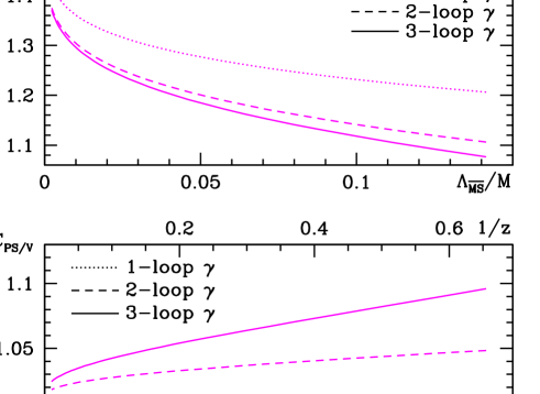
Figure 2: The functions $C_{\rm PS}$ and $C_{{\rm PS}/{\rm V}}$ evaluated in different approximations of perturbation theory. In relating $\Lambda_{\overline{{\rm MS}}}/M$ to $z=ML$, we used [41] $\Lambda_{\overline{{\rm MS}}}\,r_{0}=0.602$ and $L/r_{0}=L_{\rm max}/(2r_{0})=0.359$. (Setting $r_{0}=0.5\,{\rm fm}$, this actually corresponds to $L\approx 0.2\,{\rm fm}$.)

In order to study whether their $\alpha^{n}$-error is a limiting factor, we first note that changing the order from three-loop to four-loop in the $\beta$-function makes only a tiny difference. Next we plot $C_{\rm X}$, ${\rm X}={\rm PS,PS/V}$, using $\gamma$ at $n$ loops in figure 2. We observe a reasonable behaviour of the asymptotic perturbative series and take half of the difference between the two-loop and three-loop approximations for $\gamma$ as our uncertainty. This uncertainty will be almost negligible with respect to our statistical errors. Note that without the three-loop computations of [9] such a statement would not have been possible.

For completeness we remind the reader that eqs. (24)–(26) are afflicted by the usual problem of identifying power corrections. Asymptotically, at large $M$, the higher-order logarithmic (perturbative) corrections in $C_{\rm X}$ dominate over the $1/z^{n}$ power corrections. However, as just discussed, in the interesting range of $z$, the perturbative corrections are under reasonable control and it makes sense to investigate the power corrections if they are significantly larger. Note that this problem is not present if the effective theory is renormalized non-perturbatively [36].

3.2 Energies

Next we concentrate on the energies $\Gamma$. Clearly, because of the term $m\overline{\psi}_{\rm h}(x)\psi_{\rm h}(x)$ in the Lagrangian (1), they grow (roughly linearly) with the mass. For the case of hadron masses, mass formulae have been written down [44]; for instance, the one for the B-meson mass reads:

$$m_{\rm B}=m+\bar{\Lambda}+\frac{1}{2m}\,(\lambda_{1}+d_{\rm B}\lambda_{2})\,+\,{\rm O}\left(1/m^{2}\right)\,,\quad d_{\rm B}=3$$ (28)

(and the same formula holds for the ${\rm B}^{\ast}$-meson except that $d_{\rm B}\to d_{{\rm B}^{\ast}}=-1$). The matrix element $\lambda_{1}={\textstyle{\frac{1}{2}}}\,\omega_{\rm kin}\langle{\rm B}|-\overline{\psi}_{\rm h}{\bf D}^{2}\psi_{\rm h}|{\rm B}\rangle$ was mentioned already in the introduction, and $\lambda_{2}=\frac{1}{2d_{\rm B}}\,\omega_{\rm spin}\langle{\rm B}|-\overline{\psi}_{\rm h}{\bf\sigma}\cdot{\bf B}\,\psi_{\rm h}|{\rm B}\rangle$. Some cautioning remark concerning the above formula is in order. It suggests that the binding energy $\bar{\Lambda}=m_{\rm B}-m+{\rm O}(1/m)$ may be obtained as a prediction of HQET. However, there is no unique non-perturbative definition of the mass $m$, which should be subtracted. As a consequence, $\bar{\Lambda}$ has an ambiguity of order $\Lambda_{\rm QCD}$, which may then also propagate into a significant ambiguity in $\lambda_{1}$ extracted from eq. (28).

We nevertheless start our discussion of the effective energies $\Gamma$ from a trivial generalization of eq. (28):

$$\Gamma_{\rm av}(L,M) \equiv \frac{1}{4}\Big{[}\,\Gamma_{\rm PS}(L,M)+3\,\Gamma_{\rm V}(L,M)\,\Big{]}$$ (29)

$$= m+\bar{\Lambda}(L)+\frac{1}{2m}\,\lambda_{1}(L)\,+\,{\rm O}\left(1/m^{2}\right)\,,$$

where $\lambda_{1}(L)$ again summarizes the effect of the $\overline{\psi}_{\rm h}{\bf D}^{2}\psi_{\rm h}$-perturbation to the static action. We have cancelled a $\lambda_{2}$-term by considering the spin-averaged combination of the energy. While one ought to be careful with the interpretation of sub-leading terms in $1/M$, the large-mass behaviour of $\Gamma_{\rm av}(L,M)$ is given by

$$L\Gamma_{\rm av}(L,M)\,\raisebox{-0.43057pt}{ $\stackrel{{\scriptstyle\small{M\to\infty}}}{{\sim}}$}\,\,\,C_{\rm mass}\left(M/\Lambda_{\overline{{\rm MS}}}\right)\times z\,+\,{\rm O}\left((1/z)^{0}\right)\,,$$ (30)

with ( $\kern 1.0pt\overline{\kern-1.0ptm\kern-1.0pt}\kern 1.0pt_{\rm\overline{MS\kern-0.35002pt}\kern 0.35002pt}(\kern 1.0pt\overline{\kern-1.0ptm\kern-1.0pt}\kern 1.0pt_{*})=\kern 1.0pt\overline{\kern-1.0ptm\kern-1.0pt}\kern 1.0pt_{*}$ )

$$C_{\rm mass}\left(M/\Lambda_{\overline{{\rm MS}}}\right)={m_{Q}\over M}={\kern 1.0pt\overline{\kern-1.0ptm\kern-1.0pt}\kern 1.0pt_{*}\over M}\,{m_{Q}\over\kern 1.0pt\overline{\kern-1.0ptm\kern-1.0pt}\kern 1.0pt_{*}}$$ (31)

and $m_{Q}$ being the pole mass. Here the first factor on the right-hand side is known very precisely in perturbation theory (up to four loops [45, 46]), but it is well known that the perturbative series for the second factor is not very well behaved and even the three-loop term [47] is still rather significant. We will discuss this uncertainty in $C_{\rm mass}$ together with the numerical results in the following section.

Let us now consider the sub-leading terms in eq. (29). Taking energy differences, $m$ drops out and e.g. $\bar{\Lambda}(L)-\bar{\Lambda}(L^{\prime})$ can be computed unambiguously from the static effective theory. It does not depend on any convention adopted for $m$ in eq. (29). In our numerical computations, however, we investigated only one value of $L$. As an example of another observable unaffected by the ambiguity in $m$, we therefore look at the combination

$$\Xi(L,M)=\frac{L}{4}\left[\,\frac{f_{\rm A}^{\prime}(T/4)}{f_{\rm A}(T/4)}-\frac{f_{\rm A}^{\prime}(T/2)}{f_{\rm A}(T/2)}+3\,\frac{k_{\rm V}^{\prime}(T/4)}{k_{\rm V}(T/4)}-3\,\frac{k_{\rm V}^{\prime}(T/2)}{k_{\rm V}(T/2)}\,\right]\,.$$ (32)

The HQET prediction for this quantity is

$$\Xi(L,M)=\Xi_{\rm stat}(L)+\frac{1}{2z}\,\Xi_{\rm kin}(L)\,+\,{\rm O}\left(1/z^{2}\right)\,,$$ (33)

with

$$\Xi_{\rm stat}(L)=L\left[\,\frac{(f_{\rm A}^{\rm stat})^{\prime}(T/4)}{f_{\rm A}^{\rm stat}(T/4)}-\frac{(f_{\rm A}^{\rm stat})^{\prime}(T/2)}{f_{\rm A}^{\rm stat}(T/2)}\,\right]\,,$$ (34)

defined in the static effective theory. Since it is an energy, $\Xi$ does not require any renormalization. The first-order correction in $1/z$ is given entirely by matrix elements of $\overline{\psi}_{\rm h}(x){\bf D}^{2}\psi_{\rm h}(x)$. Its coefficient is fixed using the reparametrization invariance of the effective theory, first discussed in ref. [48]. To see this, one considers the matrix elements of $\overline{\psi}_{\rm h}(x){\bf D}^{2}\psi_{\rm h}(x)$ to be computed in dimensional regularization. Then reparametrization invariance is valid, and the coefficient of the operator renormalized by minimal subtraction is the inverse ${\rm\overline{MS\kern-0.50003pt}\kern 0.50003pt}$ quark mass [49, 50], whose renormalization scale dependence cancels against the one of the matrix element. From eq. (23) it hence follows that the prefactor of the renormalization group invariant matrix element of $\overline{\psi}_{\rm h}(x){\bf D}^{2}\psi_{\rm h}(x)$ is $1/(2M)$, as used in eq. (33). In that equation, $\Xi_{\rm kin}(L)$ is the matrix element made dimensionless by a factor $L$. In the following, the exact expression for $\Xi_{\rm kin}(L)$ will be irrelevant. It rather suffices to know that it does not depend on the mass.

We point out that, in writing down the quantum mechanical representation of $\Xi$, states play a rôle for which only the operator ${\rm e}^{-T\mathbb{H}/4}$ is effective to suppress higher energy contributions, while in our other observables ${\rm e}^{-T\mathbb{H}/2}$ suppresses high energies. For the quantity $\Xi$, HQET is thus expected to be accurate only at larger values of $z$. This variable should roughly be a factor of 2 larger than for the other observables.

Finally, in the difference

$${\Delta}_{\Gamma}(L,M)\,\equiv\,\Gamma_{\rm PS}(L,M)-\Gamma_{\rm V}(L,M)$$ (35)

the lowest-order term that contributes in the effective theory is $\overline{\psi}_{\rm h}(x){\bf\sigma}\cdot{\bf B}\,\psi_{\rm h}(x)$. With $C_{\rm spin}$ constructed from the anomalous dimension of this operator in the effective theory, $\gamma^{\rm spin}$ [51, 52], we thus have

$$L{\Delta}_{\Gamma}(L,M)\,\raisebox{-0.43057pt}{ $\stackrel{{\scriptstyle\small{M\to\infty}}}{{\sim}}$}\,\,\,C_{\rm spin}\left(M/\Lambda_{\overline{{\rm MS}}}\right)\,\frac{X_{\rm RGI}^{\rm spin}(L)}{z}\,\Big{(}1+{\rm O}(1/z)\Big{)}\,,$$ (36)

where the leading asymptotics of the function $C_{\rm spin}(M/\Lambda_{\overline{{\rm MS}}})$ is of the form

$$C_{\rm spin}\left(M/\Lambda_{\overline{{\rm MS}}}\right)\raisebox{-0.43057pt}{ $\stackrel{{\scriptstyle\small{M\to\infty}}}{{\sim}}$}\,\,\left(\ln\frac{M}{\Lambda_{\overline{{\rm MS}}}}\right)^{-\gamma_{0}^{\rm spin}/(2b_{0})}\left\{1+{\rm O}\left(\frac{\ln\left[\ln\left(M/\Lambda_{\overline{{\rm MS}}}\right)\right]}{\ln\left(M/\Lambda_{\overline{{\rm MS}}}\right)}\right)\right\}$$ (37)

with the universal coefficient (cf. appendix B)

$$\gamma_{0}^{\rm spin}=\frac{6}{(4\pi)^{2}}-d_{0}\,,$$ (38)

and $X_{\rm RGI}^{\rm spin}$ being again a renormalization group invariant matrix element, defined in the static effective theory. The relative perturbative uncertainty of $C_{\rm spin}$ is ${\rm O}(\alpha^{2})$, since here the three-loop anomalous dimension is not known. As illustrated in figure 3, the difference between the one-loop anomalous dimension and the two-loop one is tiny. Since this may, however, be accidental rather than representing the behaviour of the series, we shall take the size of the three-loop term met in $C_{\rm PS}$, figure 2, as our uncertainty. A better estimate of this uncertainty would require the knowledge of $\gamma_{2}^{\rm spin}$.

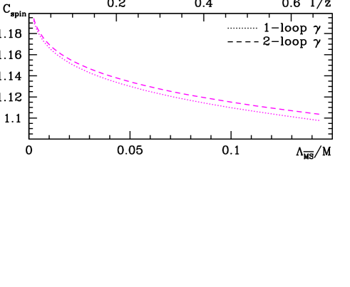
Figure 3: The function $C_{\rm spin}$ evaluated in perturbation theory.

4 Quantitative tests of the effective theory

We have tested the predictions of the effective theory applied to the quenched approximation of QCD by evaluating the observables for one geometry, namely $T=L\equiv L_{0}$, and for $\theta=0.5$. The use of the quenched approximation should not be worrying in this context, since it is of course used both in the effective theory and in QCD. Furthermore, although we set the light quark mass to zero, $1/L_{0}$ provides an infrared cutoff and there are no singularities in the chiral limit.

The numerical simulations are done on lattices with various resolutions $a/L_{0}$ followed by a continuum extrapolation. In all cases, $L_{0}$ is fixed by imposing

$$\bar{g}^{2}(L_{0}/2)=1.8811\,,$$ (39)

where $\bar{g}(L)$ is the renormalized coupling at length scale $L$ in the SF scheme [53]. It is known that $L_{0}\approx 0.2\,{\rm fm}$ [41, 36]. The (purely technical) reasons for the precise definition (39) are detailed in ref. [36]. Table 1 of ref. [35] lists the bare coupling $g_{0}$ for each resolution $L_{0}/a$, and this reference also explains how the bare quark masses are fixed to ensure a massless light quark and a prescribed value $M$ for the heavy quark.

4.1 Results in the static approximation

Some of the leading-order terms in the HQET expansions described in the previous section are known exactly due to the spin symmetry [54, 55], but for two of the expansions we have computed the non-trivial leading order from a lattice simulation in static approximation.

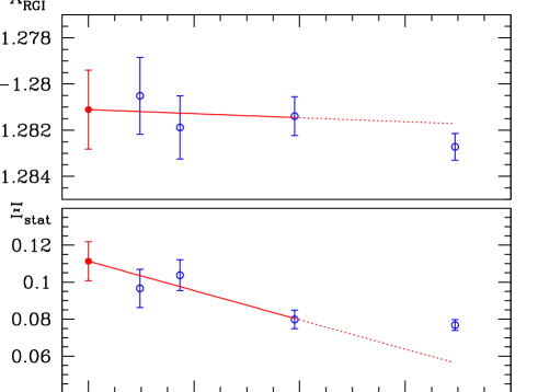
Figure 4: Continuum limit extrapolations of $X_{\rm RGI}(L_{0})$ (top) and $\Xi_{\rm stat}(L_{0})$ (bottom). The fits adopt simulation data generated with the HYP-link static quark action, see text. The $a/L$ independent part of the error of $X_{\rm RGI}$ is not included in the graph.

The first one is the matrix element of the time component of the axial current, $X_{\rm RGI}(L)$ in eq. (21). Indicating explicitly also the dependence on the bare coupling $g_{0}$ and the lattice spacing $a$, it is given by

$$X_{\rm RGI}(L_{0})=\lim_{a/L_{0}\to 0}Z_{\rm RGI}(g_{0})\,X(g_{0},L_{0}/a)\,.$$ (40)

From the relation of $X$ to the very definition of the renormalization factor $Z_{\rm RGI}$, as detailed in ref. [39], one obtains the explicit form

$$Z_{\rm RGI}\,X=\frac{\Phi_{\rm RGI}}{\Phi(\mu=1/L_{0})}\times\left.\frac{\left(f_{1}^{\rm hh}\,f_{1}\right)^{1/4}}{\sqrt{f_{1}^{\rm stat}}}\right|_{L=L_{0}}\times\left[\,X\,\right]_{\,{\rm tree-level}}$$ (41)

for the right-hand side of eq. (40). All quantities that enter the above expression have been defined in the latter reference. For its numerical evaluation we take the non-perturbatively ${\rm O}(a)$ improved action of [40] for the light quarks and the improved discretizations of [56] for the heavy quark. We note in passing that, using the data of [39], we first evaluated this quantity with the Eichten-Hill action for the heavy quark [1]. However, this resulted in an order of magnitude larger error for $X_{\rm RGI}$ at $L_{0}/a=32$.

The limit $a/L_{0}\to 0$ is taken by a linear fit in $(a/L_{0})^{2}$ as illustrated in the upper diagram of figure 4, referring to the data set from a simulation with the static quark action built from HYP-links [57, 56]. We quote the result from a fit with $L_{0}/a\geq 16$ as our continuum result,

$$X_{\rm RGI}(L_{0})=-1.281(9)\,,$$ (42)

which also receives an error contribution from the (regularization independent) factor $\Phi_{\rm RGI}/\Phi(1/L_{0})$ in eq. (41) [39]. Including all points with $L_{0}/a\geq 12$ in the fit yields a compatible continuum value with smaller error. In the same way we obtain (cf. eq. (34) and the lower diagram of figure 4):

$$\Xi_{\rm stat}(L_{0})=0.11(1)\,.$$ (43)

4.2 Results at finite $M$ and comparison

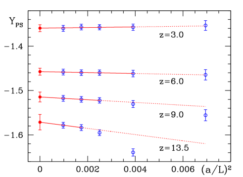
Figure 5: Continuum extrapolations for some $z$-values spanning the entire range of $z$. The linear fit in $(a/L)^{2}$ is shown by the full line and extended also to those values of $a/L$ that did not participate in the fit by a dotted line.

The finite-mass (quenched) QCD observables are obtained from similar extrapolations of lattice results at finite $a/L$. However, as the variable $z$ is increased, the quark mass in lattice units grows at a given resolution $a/L$. A perturbative computation [14] as well as our non-perturbative study suggest that ${\rm O}(a)$ improvement may be trusted only below a certain value of the quark mass in lattice units. It is therefore necessary to impose a cut on the quark mass. For a given $z$, this cut translates into estimates of the coarsest lattice resolutions beyond which the lattice data are to be omitted from the continuum extrapolations. As in ref. [35] we impose $aM<0.6$ and follow this reference on all other details of the lattice computations as well as the extraction of the continuum limits. For illustration we just show the continuum extrapolations of $Y_{\rm PS}(L,M)$, $L=L_{0}$, at selected values of $z$ in figure 5. In addition we mention a few features equally true for the continuum limit extrapolations of the other observables, which enter our investigation but are not shown in figures.

• The slopes in $a/L$ are rather small.

• The error in the continuum limit grows with $z$, because less lattices can be used in the extrapolation at large $z$.

• The continuum limit is compatible with the values at the smallest two lattice spacings. Its error is conservative.

In appendix A we collect our numerical results both at finite lattice spacing and in the continuum limit.

		Linear					Quadratic
Quantity		$a_{0}$		$a_{1}$			$a_{0}$		$a_{1}$		$a_{2}$
$z$-range: $3.0$–$13.5$
$Y_{\rm PS}/C_{\rm PS}$							$-1$.	$281(7)$	$0$.	$64(8)$	$-1$.	$0(2)$
$Y_{\rm V}/C_{\rm V}$							$-1$.	$281(7)$	$-0$.	$63(9)$	$0$.	$3(2)$
$R/C_{{\rm PS}/{\rm V}}$							$1$.	$0$	$-0$.	$89(1)$	$1$.	$06(3)$
$L\Gamma_{\rm av}/(z\,C_{\rm mass})$							$1$.	$0$	$0$.	$42(3)$	$0$.	$14(10)$
$L{\Delta}_{\Gamma}/C_{\rm spin}$							$0$.	$0$	$-1$.	$69(6)$	$0$.	$8(2)$
$\Xi$							$0$.	$109(8)$	$0$.	$7(1)$	$-0$.	$8(3)$
$z$-range: $5.15$–$13.5$
$Y_{\rm PS}/C_{\rm PS}$		$-1$.	$277(7)$	$0$.	$45(4)$		$-1$.	$281(8)$	$0$.	$7(1)$	$-1$.	$3(5)$
$Y_{\rm V}/C_{\rm V}$		$-1$.	$281(9)$	$-0$.	$59(6)$		$-1$.	$281(7)$	$-0$.	$6(1)$	$0$.	$2(6)$
$R/C_{{\rm PS}/{\rm V}}$		$1$.	$0$	$-0$.	$722(7)$		$1$.	$0$	$-0$.	$91(1)$	$1$.	$18(5)$
$L\Gamma_{\rm av}/(z\,C_{\rm mass})$		$1$.	$0$	$0$.	$44(2)$		$1$.	$0$	$0$.	$41(6)$	$0$.	$2(3)$
$L{\Delta}_{\Gamma}/C_{\rm spin}$		$0$.	$0$	$-1$.	$56(4)$		$0$.	$0$	$-1$.	$62(6)$	$0$.	$4(2)$
$\Xi$		$0$.	$112(8)$	$0$.	$54(7)$		$0$.	$110(9)$	$0$.	$6(2)$	$-0$.	$5(7)$

Table 1: Fit parameters describing the $z$-dependences of the form $a_{0}+a_{1}/z+a_{2}/z^{2}$. Where the constant term, $a_{0}$, is listed without an error, it is constrained to the prediction of the static effective theory. (In case of the entire $z$-range, only the quadratic fit results are given.) All these fits have an acceptable goodness-of-fit.

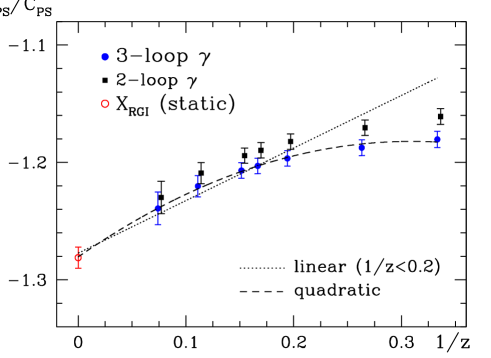
Figure 6: The ratio $Y_{\rm PS}(L,M)/C_{\rm PS}(M/\Lambda_{\overline{{\rm MS}}})$ with $C_{\rm PS}$ using the two- and the three-loop anomalous dimension of the static axial current. Error bars do not contain the perturbative uncertainty in $C_{\rm PS}$. The fits shown refer to the three-loop evaluation of $C_{\rm PS}$ and include the result for $X_{\rm RGI}$ in the static limit. (Points using only the two-loop anomalous dimension are slightly displaced here.)

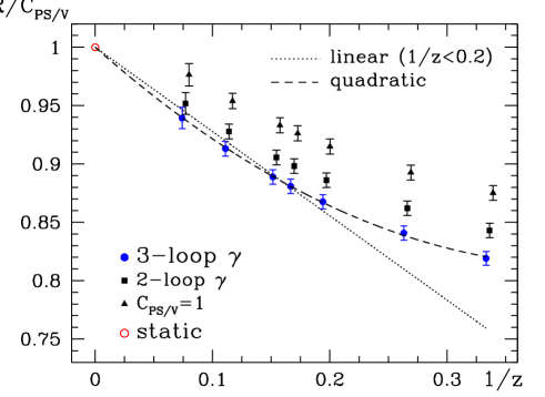
Figure 7: As in figure 6. The fits use the evaluation of $C_{{\rm PS}/{\rm V}}$ with the two-loop matching coefficient between HQET and QCD; they are constrained to the prediction of the static effective theory. (On the level of perturbative orders, two-loop matching belongs to the three-loop anomalous dimension of the currents, cf. appendix B).

We are now ready to compare the continuum results with the predictions of HQET. Before that, we remind the reader that energies of order $2/L$ still contribute significantly to our observables. It is thus possible that the $1/M$-expansion breaks down earlier in our finite-volume situation than it does in large volume. However, our numerical results do not give any indication of such a behaviour.

Let us start with the current matrix elements. The prediction for the matrix element of the axial current is $Y_{\rm PS}(L,M)/C_{\rm PS}=X_{\rm RGI}(L)+{\rm O}(1/z)$. In this combination, plotted in figure 6, the perturbatively computed coefficient $C_{\rm PS}(M/\Lambda_{\overline{{\rm MS}}})$ compensates a significant part of the mass dependence of $Y_{\rm PS}$. The finite-mass $Y_{\rm PS}/C_{\rm PS}$ is obviously well compatible with approaching the static result, eq. (42), as $1/z\to 0$. To quantify the deviations from the static limit at finite $z$, we fit all data points, including $1/z=0$, to first- and second-order polynomials in $1/z$:

$$\frac{Y_{\rm PS}}{C_{\rm PS}}\,=\,a_{0}\,+\,\frac{a_{1}}{z}\,+\,\ldots\,\,.$$ (44)

In these fits also the uncertainty in $C_{\rm PS}$ is taken into account (i.e. half of the difference between $C_{\rm PS}$ evaluated with the two-loop and three-loop anomalous dimension). We perform them separately to the data in the range $1/z<0.2$, which means masses around the b-quark mass and higher [36], and over the whole range, see table 1. Comparing $a_{1}$ obtained from the quadratic fit over the whole range ($z=3.0$–$13.5$) and the linear fit for $1/z<0.2$ ($z\geq 5.15$), the change is not so small. This indicates that a precise identification of the first-order correction is not possible with our precision and range of $z$. However, the rough magnitude of $a_{1}\approx 0.6$ can be inferred and, more importantly, it is clear that the overall magnitude of $1/z$-corrections is reasonably small. It is also relevant to remember that eq. (44) is only an approximate parametrization of the $z$-dependence, since the renormalization of the higher-dimensional operators in the effective theory will introduce logarithmic modifications of the simple power series. It is thus conceivable that these logarithms account for some of the curvature seen in figure 6.

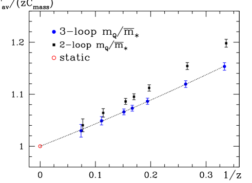
Figure 8: Quadratic fit over the entire $z$-range of the combination $L\Gamma_{\rm av}/(z\,C_{\rm mass})$, which is constrained to approach 1 in the static limit. It employs the three-loop relation between the pole and the $\overline{\rm MS}$ mass; the results using this relation to only two loops are also depicted for comparison.

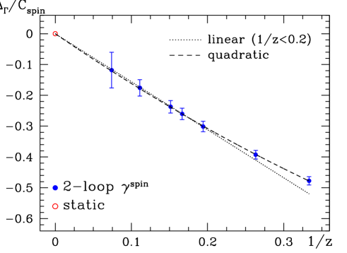
Figure 9: Fits in $1/z$ constrained to the static result and referring to the two-loop evaluation of $C_{\rm spin}$. The linear fit is only based on the heavier quark mass points with $z=5.15$–$13.5$, while the quadratic one (i.e. also allowing for a $1/z^{2}$-term) includes all points.

For the ratio of matrix elements $R(L,M)$, eq. (26), the lowest-order term in the $1/z$-expansion is fixed to be 1 by the spin symmetry of the static theory. As is reflected by figure 7, the results at finite $1/z$ are well compatible with this, if the function $C_{{\rm PS}/{\rm V}}$ is evaluated including at least the two-loop anomalous dimensions. Fits to $R/C_{{\rm PS}/{\rm V}}$ are performed in complete analogy to eq. (44). The corresponding parameters of table 1 are again of order unity. In that table we also include the parameters of the analogous fits to the quantity $Y_{\rm V}/C_{\rm V}$.

Turning our attention to the effective energies, introduced in section 2.1, a first rough test of HQET is the behaviour of the spin-averaged energy $\Gamma_{\rm av}$. Figure 8 confirms the expectation that the combination $L\Gamma_{\rm av}/(z\,C_{\rm mass})$ approaches 1 up to $1/z$-corrections as $1/z\to 0$ (see eq. (30)). Note that the $(1/z)^{2}$-corrections in $\Gamma_{\rm av}$ are very small, which is of particular interest for the computation of the b-quark mass in static approximation [36, 35]. There the quantity $\Gamma_{\rm av}$ was used in order to non-perturbatively match the quark mass of the effective theory to the one in QCD. The dominant error in the final estimate for the quark mass, $M_{\rm b}$, is expected to originate from this matching and is of order $M_{\rm b}\times(1/z)^{2}$. From the values of $a_{2}$ and $z_{\rm b}\equiv m_{\rm b}L\approx 5$, we may estimate the relative error to be roughly of the order of $0.2\times(1/5)^{2}\approx 1\%$. As seen from the figure, this conclusion is not very much affected either by the perturbative uncertainty visible in the graph as a difference between the two-loop and three-loop approximations for the pole mass $m_{Q}$ in eq. (31); the $1/z^{2}$-curvature is not very different.

The spin splitting ${\Delta}_{\Gamma}(L,M)$, which vanishes in the static limit, is displayed in figure 9. It is in good agreement with the HQET prediction but exhibits a rather large $1/z$-coefficient.

Finally, we successfully test eq. (33) in figure 10. Recall that a simple kinematical consideration leads one to expect the $1/z$-expansion to only be applicable at smaller values of $1/z$ for this observable (cf. section 3.2). On the other hand, reparametrization invariance allows to exclude logarithmic modifications of the $1/z$-term; in contrast to our other tests, figure 10 does not involve any perturbative conversion factor.

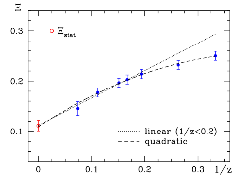
Figure 10: Linear and quadratic fits of the observable $\Xi$ as in figures 6–9, where the static data point, $\Xi_{\rm stat}$, is included in the fits.

5 Conclusions

All of the comparisons of QCD observables with the predictions of HQET discussed in this work represent tests of the effective theory, which it passed successfully. As a significant improvement of earlier non-perturbative (lattice) tests, these comparisons are performed after first taking the continuum limit of the non-perturbatively renormalized quantities. Thus, worries that ${\rm O}(a)$ effects, in particular those that grow with the quark mass, may afflict the large-mass behaviour in QCD are removed.

For a precise judgement of figures 6–10 it is important to be aware of the level of precision of renormalization and matching. The renormalization problem of the static axial current has been solved non-perturbatively in [39] and with this information all points at $1/z=0$ are known without any residual perturbative uncertainty. For the quantity $\Xi$ shown in figure 10, this is also true at finite $1/z$. However, in general we need to know the functions $C_{\rm X}$, which relate the QCD observables at finite mass $M$ (and thus finite $z=ML$) to the renormalization group invariants of the effective theory, such as $X_{\rm RGI}$ in figure 6. While the latter are unambiguously defined and have been computed non-perturbatively, the former are known only in perturbation theory and have errors of order $\alpha^{n}$, with $\alpha$ evaluated at the scale of the heavy quark mass. We have discussed these errors. On a phenomenological level they are under control due to the computations [58, 9], except for $C_{\rm spin}$, where a next-to-next-to-leading-order computation is not yet available. Still, one should remember that – strictly speaking – the isolation of $1/m$-corrections by looking at the difference to the leading-order HQET result is only possible when $C_{\rm X}$ is known non-perturbatively: parametrically, ${\rm O}([\alpha(m)]^{n})$ corrections are always larger than ${\rm O}(1/m)$. Nevertheless, our results in figures 6–10 are compatible with the $z^{-n}$ power corrections dominating over the perturbative ones in the accessible range of $z$. Fitting them by a simple polynomial in $1/z$, the coefficients turn out to be of order 1 as naively expected. Therefore, at the b-quark mass, which corresponds to $z_{\rm b}\equiv m_{\rm b}L\approx 5$ for our value of $L=L_{0}\approx 0.2\,{\rm fm}$, the effective theory is very useful.

Beyond the general interest of providing a non-perturbative test for HQET, these results are important for the programme of ref. [36]. There it was suggested to determine the $1/m_{\rm b}$-corrections to B-physics matrix elements from a simulation of HQET on the lattice. The coefficients $c_{k}$ of the various terms in the HQET Lagrangian and of the effective composite fields are to be determined by matching HQET and QCD in a finite volume, and it was proposed to employ a value of $L$ similar to $L_{0}$ in this step. This value has to be large enough such that (i) $z_{\rm b}$ is in the range where HQET is applicable with small corrections, yet (ii) $L_{0}$ has to be small enough to allow for the computation of the QCD observables at $m=m_{\rm b}$ with small $a$-effects. From table 1 we conclude that $L=L_{0}$ is indeed promising. In fact, in the previous section we roughly estimated that the correction to the static limit computation of the RGI b-quark mass [34, 36] is only of the order of $1\%$.

However, this application appears to be a particularly favourable case and it would be of advantage to have a larger value of $z_{\rm b}$ (i.e. larger $L$) in the matching step to suppress higher-order terms. Our analysis suggests that this is indeed possible, since we may determine QCD observables rather precisely in, say, the entire range $z\geq 5$ by combining QCD results at finite $z$ with the static limit. Choosing, for instance, $L\approx 2L_{0}$ in the matching step, one needs the QCD observables for $z\approx 10$. The errors of the quadratic fit functions evaluated at $z=z_{{\rm b}}=10$ are typically 30%–50% smaller than the errors of the neighbouring points seen in figures 6–10. Proceeding in this way, namely taking the fit functions as representations of the QCD observables in finite volume (of course within their errors), one may obtain the HQET parameters as functions of the quark mass and infer predictions for all quark masses larger than the minimal one considered. With the entire matching done non-perturbatively, the final HQET results will differ from QCD by ${\rm O}(1/m^{2})$ if $1/m$-terms are properly included. No perturbative errors as in $C_{\rm X}$ enter in this programme.

We finally remind the reader that in the quantities discussed in this paper, as well as in the matching step just described, we are dealing with matrix elements of a mixture of energy eigenstates where states with energy of ${\rm O}(1/L)$ contribute. Hence the $1/m$-expansion for the large-volume B-physics matrix elements may be expected to behave even better and should be well under control, once this is the case for the matching step.

Appendix A Results at finite lattice spacing

For any details on the lattice simulations and the subsequent analysis of the numerical data, the reader is referred to [35] and references therein. In table 2 we therefore directly list the results on the observables studied in this work at finite values of the lattice spacing as well as in the continuum limit. As already mentioned in section 4, the latter have been extracted by linear extrapolations $(a/L)^{2}\rightarrow 0$ of the ${\rm O}(a)$ improved lattice data following the same procedure as adopted in ref. [35].

$L/a$		$Y_{\rm PS}(L,M)$		$Y_{\rm V}(L,M)$		$R(L,M)$		$L{\Delta}_{\Gamma}(L,M)$		$\Xi(L,M)$
$z=3.0$
$12$		$-1$.	$35(1)$	$-1$.	$581(7)$	$0$.	$869(8)$	$-0$.	$509(10)$	$0$.	$245(4)$
$16$		$-1$.	$357(7)$	$-1$.	$576(7)$	$0$.	$874(6)$	$-0$.	$512(10)$	$0$.	$256(5)$
$20$		$-1$.	$357(6)$	$-1$.	$575(7)$	$0$.	$875(5)$	$-0$.	$521(11)$	$0$.	$259(6)$
$24$		$-1$.	$357(6)$	$-1$.	$576(7)$	$0$.	$874(5)$	$-0$.	$522(13)$	$0$.	$259(8)$
$32$		$-1$.	$360(7)$	$-1$.	$577(7)$	$0$.	$875(5)$	$-0$.	$533(14)$	$0$.	$246(9)$
CL		${\it-1}$.	${\it 359(8)}$	${\it-1}$.	${\it 576(8)}$	${\it 0}$.	${\it 875(6)}$	${\it-0}$.	${\it 537(15)}$	${\it 0}$.	${\it 250(9)}$
$z=3.8$
$12$		$-1$.	$39(1)$	$-1$.	$591(7)$	$0$.	$884(8)$	$-0$.	$419(13)$	$0$.	$226(4)$
$16$		$-1$.	$392(7)$	$-1$.	$584(7)$	$0$.	$890(6)$	$-0$.	$423(12)$	$0$.	$240(5)$
$20$		$-1$.	$391(6)$	$-1$.	$582(7)$	$0$.	$892(5)$	$-0$.	$430(12)$	$0$.	$240(6)$
$24$		$-1$.	$391(6)$	$-1$.	$582(7)$	$0$.	$891(5)$	$-0$.	$431(13)$	$0$.	$241(8)$
$32$		$-1$.	$394(7)$	$-1$.	$583(7)$	$0$.	$892(5)$	$-0$.	$441(15)$	$0$.	$228(9)$
CL		${\it-1}$.	${\it 394(8)}$	${\it-1}$.	${\it 581(8)}$	${\it 0}$.	${\it 893(6)}$	${\it-0}$.	${\it 444(16)}$	${\it 0}$.	${\it 232(9)}$
$z=5.15$
$12$		$-1$.	$44(1)$	$-1$.	$609(7)$	$0$.	$904(8)$	$-0$.	$315(17)$	$0$.	$200(4)$
$16$		$-1$.	$438(7)$	$-1$.	$596(7)$	$0$.	$910(6)$	$-0$.	$320(15)$	$0$.	$215(5)$
$20$		$-1$.	$437(6)$	$-1$.	$592(7)$	$0$.	$913(5)$	$-0$.	$328(15)$	$0$.	$216(6)$
$24$		$-1$.	$437(6)$	$-1$.	$591(7)$	$0$.	$913(5)$	$-0$.	$327(16)$	$0$.	$218(8)$
$32$		$-1$.	$436(7)$	$-1$.	$589(7)$	$0$.	$914(5)$	$-0$.	$341(17)$	$0$.	$210(9)$
CL		${\it-1}$.	${\it 435(8)}$	${\it-1}$.	${\it 586(8)}$	${\it 0}$.	${\it 915(6)}$	${\it-0}$.	${\it 343(19)}$	${\it 0}$.	${\it 214(9)}$

Table 2: Lattice results on the quantities of this work for different values of the dimensionless renormalization group invariant heavy quark mass, $z=ML$, with $L\equiv L_{0}\approx 0.2\,{\rm fm}$. The full sets of simulation parameters can be inferred from tables 1 and 4 of ref. [35], where also the results for $L\Gamma_{\rm av}$ were published. The quoted errors cover the statistical as well as the systematic uncertainties, including those originating from the fact that in the numerical simulations $z$ can only be fixed within some finite precision. Continuum limits are displayed in italics.

$L/a$		$Y_{\rm PS}(L,M)$		$Y_{\rm V}(L,M)$		$R(L,M)$		$L{\Delta}_{\Gamma}(L,M)$		$\Xi(L,M)$
$z=6.0$
$12$		$-1$.	$46(1)$	$-1$.	$620(7)$	$0$.	$913(8)$	$-0$.	$270(20)$	$0$.	$186(4)$
$16$		$-1$.	$462(7)$	$-1$.	$604(7)$	$0$.	$920(6)$	$-0$.	$276(17)$	$0$.	$203(5)$
$20$		$-1$.	$460(6)$	$-1$.	$597(7)$	$0$.	$923(5)$	$-0$.	$283(17)$	$0$.	$205(6)$
$24$		$-1$.	$460(6)$	$-1$.	$595(7)$	$0$.	$924(5)$	$-0$.	$282(17)$	$0$.	$207(8)$
$32$		$-1$.	$458(7)$	$-1$.	$593(7)$	$0$.	$924(5)$	$-0$.	$296(19)$	$0$.	$198(9)$
CL		${\it-1}$.	${\it 457(8)}$	${\it-1}$.	${\it 589(8)}$	${\it 0}$.	${\it 926(6)}$	${\it-0}$.	${\it 297(21)}$	${\it 0}$.	${\it 203(9)}$
$z=6.6$
$12$		$-1$.	$48(1)$	$-1$.	$629(7)$	$0$.	$918(8)$	$-0$.	$243(21)$	$0$.	$178(4)$
$16$		$-1$.	$477(8)$	$-1$.	$609(7)$	$0$.	$926(6)$	$-0$.	$251(19)$	$0$.	$196(5)$
$20$		$-1$.	$474(6)$	$-1$.	$601(7)$	$0$.	$930(5)$	$-0$.	$258(19)$	$0$.	$198(6)$
$24$		$-1$.	$474(6)$	$-1$.	$599(7)$	$0$.	$930(5)$	$-0$.	$257(19)$	$0$.	$201(8)$
$32$		$-1$.	$473(7)$	$-1$.	$596(7)$	$0$.	$931(5)$	$-0$.	$270(20)$	$0$.	$191(9)$
CL		${\it-1}$.	${\it 471(8)}$	${\it-1}$.	${\it 591(8)}$	${\it 0}$.	${\it 933(6)}$	${\it-0}$.	${\it 271(23)}$	${\it 0}$.	${\it 197(9)}$
$z=9.0$
$12$		$-1$.	$56(1)$	$-1$.	$678(7)$	$0$.	$933(8)$	$-0$.	$166(31)$	$0$.	$149(4)$
$16$		$-1$.	$530(8)$	$-1$.	$633(7)$	$0$.	$943(6)$	$-0$.	$182(27)$	$0$.	$172(5)$
$20$		$-1$.	$522(6)$	$-1$.	$618(7)$	$0$.	$948(5)$	$-0$.	$190(25)$	$0$.	$176(6)$
$24$		$-1$.	$520(6)$	$-1$.	$612(7)$	$0$.	$950(5)$	$-0$.	$189(25)$	$0$.	$180(8)$
$32$		$-1$.	$517(7)$	$-1$.	$608(7)$	$0$.	$951(5)$	$-0$.	$200(26)$	$0$.	$170(9)$
CL		${\it-1}$.	${\it 515(11)}$	${\it-1}$.	${\it 600(12)}$	${\it 0}$.	${\it 954(7)}$	${\it-0}$.	${\it 202(30)}$	${\it 0}$.	${\it 177(9)}$
$z=13.5$
$16$		$-1$.	$639(8)$	$-1$.	$713(7)$	$0$.	$961(6)$	$-0$.	$106(47)$	$0$.	$139(5)$
$20$		$-1$.	$595(7)$	$-1$.	$659(7)$	$0$.	$967(5)$	$-0$.	$123(39)$	$0$.	$149(5)$
$24$		$-1$.	$583(7)$	$-1$.	$640(7)$	$0$.	$970(6)$	$-0$.	$126(37)$	$0$.	$157(8)$
$32$		$-1$.	$578(7)$	$-1$.	$631(7)$	$0$.	$973(6)$	$-0$.	$132(39)$	$0$.	$142(9)$
CL		${\it-1}$.	${\it 571(17)}$	${\it-1}$.	${\it 619(18)}$	${\it 0}$.	${\it 976(9)}$	${\it-0}$.	${\it 137(66)}$	${\it 0}$.	${\it 145(14)}$

Table 3: (continued).

Appendix B Perturbative conversion factors between QCD and HQET

In this appendix we provide details on the numerical evaluation of the perturbative approximations of the conversion functions $C_{\rm X}(M/\Lambda_{\rm\overline{MS}})$ (${\rm X=PS,V,PS/V,spin}$) that translate the matrix elements and energies obtained in the effective theory to those in quenched QCD at finite values of the heavy quark mass. Also the case of the conversion factor $C_{\rm mass}(M/\Lambda_{\rm\overline{MS}})$, which relates the heavy quark’s pole mass $m_{Q}$ to the renormalization group invariant quark mass $M$, will be addressed.

Let us begin with the definition of the conversion functions for matrix elements of the heavy-light currents. Parametrized with the $\overline{\rm MS}$ mass $\kern 1.0pt\overline{\kern-1.0ptm\kern-1.0pt}\kern 1.0pt_{\ast}$, implicitly defined through

$$\kern 1.0pt\overline{\kern-1.0ptm\kern-1.0pt}\kern 1.0pt_{\rm\overline{MS\kern-0.35002pt}\kern 0.35002pt}(\kern 1.0pt\overline{\kern-1.0ptm\kern-1.0pt}\kern 1.0pt_{\ast})=\kern 1.0pt\overline{\kern-1.0ptm\kern-1.0pt}\kern 1.0pt_{\ast}\,,$$ (45)

we write them for ${\rm X=\rm PS}$ and V as

$$\widehat{C}_{\rm X}(\kern 1.0pt\overline{\kern-1.0ptm\kern-1.0pt}\kern 1.0pt_{\ast})\equiv\left[\,2b_{0}\bar{g}^{2}(\kern 1.0pt\overline{\kern-1.0ptm\kern-1.0pt}\kern 1.0pt_{\ast})\,\right]^{\gamma_{0}^{\rm X}/(2b_{0})}\exp\left\{\int\limits_{0}^{\bar{g}(\kern 1.0pt\overline{\kern-1.0ptm\kern-1.0pt}\kern 1.0pt_{\ast})}{\rm d}g\left[\,\frac{\gamma^{\rm X}(g)}{\beta(g)}-\frac{\gamma_{0}^{\rm X}}{b_{0}g}\,\right]\right\}.$$ (46)

Here, $\beta(g)=-g^{3}b_{0}-g^{5}b_{1}+\ldots$ is the four-loop anomalous dimension [43] of the renormalized coupling $\bar{g}(\mu)$ in the $\rm\overline{MS}$ scheme with the leading- and next-to-leading-order coefficients $b_{0}={11}/{(4\pi)^{2}}$ and $b_{1}=102/(4\pi)^{4}$. In eq. (46) we have introduced the anomalous dimensions in the matching scheme

$$\gamma^{\rm X}(g)=-g^{2}\left\{\,\gamma_{0}^{\rm X}+\gamma_{1}^{\rm X}g^{2}+\gamma_{2}^{\rm X}g^{4}+\ldots\,\right\}\,.$$ (47)

At one-loop order they are the universal ones [60, 61],

$$\gamma_{0}^{\rm PS}=\gamma_{0}^{\rm V}=-\frac{1}{4\pi^{2}}\,,$$ (48)

and at higher order they are related to the anomalous dimensions $\gamma^{\rm X,\,{\rm\overline{MS\kern-0.35002pt}\kern 0.35002pt}}(g)$ of the corresponding effective theory operator in the $\overline{\rm MS}$ scheme via

$$\gamma_{1}^{\rm X} = \gamma_{1}^{\rm X,\,{\rm\overline{MS\kern-0.35002pt}\kern 0.35002pt}}+2b_{0}c_{1}^{\rm X}\,,$$ (49)

$$\gamma_{2}^{\rm X} = \gamma_{2}^{\rm X,\,{\rm\overline{MS\kern-0.35002pt}\kern 0.35002pt}}+4b_{0}(c_{2}^{\rm X}+\gamma_{0}^{\rm X}k)+2b_{1}c_{1}^{\rm X}-2b_{0}[c_{1}^{\rm X}]^{2}\,.$$ (50)

For ${\rm X=PS}$ and V, the $\overline{\rm MS}$ two-loop anomalous dimensions are known from [62, 63, 64] and the three-loop ones from ref. [9]. The coefficients

$$c_{1}^{\rm PS}=-{2\over 3}\,{1\over 4\pi^{2}}\,, c_{2}^{\rm PS}=-4.2\,{1\over(4\pi^{2})^{2}}\,,$$ (51)

$$c_{1}^{\rm V}=-{4\over 3}\,{1\over 4\pi^{2}}\,, c_{2}^{\rm V}=-11.5\,{1\over(4\pi^{2})^{2}}$$ (52)

originate from the matching of the effective theory operators renormalized in the ${\rm\overline{MS\kern-0.50003pt}\kern 0.50003pt}$ scheme to the physical ones in QCD [1, 65, 58], while the term proportional to

$$k=-{1\over 3\pi^{2}}\,$$ (53)

is due to a reparametrization: the matching was originally done at the matching scale expressed in terms of the heavy quark’s pole mass, $m_{Q}$. Using the perturbative expansion for the ratio $\kern 1.0pt\overline{\kern-1.0ptm\kern-1.0pt}\kern 1.0pt_{\ast}/m_{Q}$ [66],

$$\frac{\kern 1.0pt\overline{\kern-1.0ptm\kern-1.0pt}\kern 1.0pt_{\ast}}{m_{Q}}=1+k\,\bar{g}^{2}(\kern 1.0pt\overline{\kern-1.0ptm\kern-1.0pt}\kern 1.0pt_{\ast})+\ldots\,,$$ (54)

the pole mass can be replaced by $\kern 1.0pt\overline{\kern-1.0ptm\kern-1.0pt}\kern 1.0pt_{\ast}$.

Next, we turn to the chromomagnetic operator $\overline{\psi}_{\rm h}{\bf\sigma}\cdot{\bf B}\,\psi_{\rm h}$. If, for the moment, we follow the common practice that in the HQET expansion its matrix element is understood to multiply the inverse pole mass, $1/m_{Q}$, the associated conversion function $\widehat{C}_{\rm mag}$ would be given by eq. (46) with an expansion (47) for ${\rm X=mag}$ and the universal one-loop coefficient [67, 68]

$$\gamma_{0}^{\rm mag}=\frac{6}{(4\pi)^{2}}\,.$$ (55)

With the two-loop anomalous dimension $\gamma_{1}^{\rm mag,\,{\rm\overline{MS\kern-0.35002pt}\kern 0.35002pt}}$ in the effective theory given in [51, 52] one finds

$$\gamma_{1}^{\rm mag}=\gamma_{1}^{\rm mag,\,{\rm\overline{MS\kern-0.35002pt}\kern 0.35002pt}}+2b_{0}c_{1}^{\rm mag}\,,\quad c_{1}^{\rm mag}={13\over 6}\,{1\over 4\pi^{2}}\,,$$ (56)

where $c_{1}^{\rm mag}$ was determined in [67]. In view of eq. (36), however, we are rather interested in a function $C_{\rm spin}$, which multiplies $1/M$. In other words, the conversion function $\widehat{C}_{\rm spin}$ must also include the factors $\kern 1.0pt\overline{\kern-1.0ptm\kern-1.0pt}\kern 1.0pt_{\ast}/m_{Q}$ and $M/\kern 1.0pt\overline{\kern-1.0ptm\kern-1.0pt}\kern 1.0pt_{\ast}$ in order to cancel the conventional factor $1/m_{Q}$ in the HQET expansion in favour of $1/M$. Using the relation

$$\frac{M}{\kern 1.0pt\overline{\kern-1.0ptm\kern-1.0pt}\kern 1.0pt_{\ast}}=\left[\,2b_{0}\bar{g}^{2}(\kern 1.0pt\overline{\kern-1.0ptm\kern-1.0pt}\kern 1.0pt_{\ast})\,\right]^{-d_{0}/(2b_{0})}\exp\left\{-\int\limits_{0}^{\bar{g}(\kern 1.0pt\overline{\kern-1.0ptm\kern-1.0pt}\kern 1.0pt_{\ast})}{\rm d}g\left[\,\frac{\tau(g)}{\beta(g)}-\frac{d_{0}}{b_{0}g}\,\right]\right\}\,,$$ (57)

where $\tau(g)=-g^{2}d_{0}-g^{4}d_{1}+\ldots$ denotes the quark mass anomalous dimension in the ${\rm\overline{MS\kern-0.50003pt}\kern 0.50003pt}$ scheme in QCD (known up to four loops [45, 46] with leading coefficient $d_{0}=8/(4\pi)^{2}$), and the ratio (54), we then obtain eqs. (46) and (47) for ${\rm X=spin}$ and

$$\gamma_{0}^{\rm spin} = \gamma_{0}^{\rm mag}-d_{0}=\frac{6}{(4\pi)^{2}}-d_{0}\,,$$ (58)

$$\gamma_{1}^{\rm spin} = \gamma_{1}^{\rm mag}-d_{1}+2b_{0}k=\gamma_{1}^{\rm mag,\,{\rm\overline{MS\kern-0.35002pt}\kern 0.35002pt}}-d_{1}+2b_{0}(c_{1}^{\rm mag}+k)\,,$$ (59)

with $\gamma_{1}^{\rm mag}$ from eq. (56).

For the special case of the ratio of pseudoscalar and vector current matrix elements, ${\rm X=PS/V}$, all but the contributions from the matching cancel and one gets

$$\widehat{C}_{\rm PS/V}(\kern 1.0pt\overline{\kern-1.0ptm\kern-1.0pt}\kern 1.0pt_{\ast})\equiv\exp\left\{\int\limits_{0}^{\bar{g}(\kern 1.0pt\overline{\kern-1.0ptm\kern-1.0pt}\kern 1.0pt_{\ast})}{\rm d}g\,\,\frac{\gamma^{\rm PS}(g)-\gamma^{\rm V}(g)}{\beta(g)}\right\}\,.$$ (60)

To parametrize the mass dependence of energy observables (such as $\Gamma_{\rm av}$ in eq. (29) of section 3.2), we also define

$$\widehat{C}_{\rm mass}(\kern 1.0pt\overline{\kern-1.0ptm\kern-1.0pt}\kern 1.0pt_{\ast})\equiv{m_{Q}\over\kern 1.0pt\overline{\kern-1.0ptm\kern-1.0pt}\kern 1.0pt_{\ast}}\,{\kern 1.0pt\overline{\kern-1.0ptm\kern-1.0pt}\kern 1.0pt_{\ast}\over M}\,,$$ (61)

where in this case the highest available perturbative precision is achieved by taking the four-loop $\tau$-function [45, 46] in $\kern 1.0pt\overline{\kern-1.0ptm\kern-1.0pt}\kern 1.0pt_{\ast}/M$ together with the three-loop expression for $m_{Q}/\kern 1.0pt\overline{\kern-1.0ptm\kern-1.0pt}\kern 1.0pt_{\ast}$ [47].

Finally, changing the argument of the various $\widehat{C}_{X}$ to the renormalization group invariant ratio $M/\Lambda_{\rm\overline{MS}}$ via (57), we straightforwardly arrive at the conversion functions

$$C_{\rm X}\left(M/\Lambda_{{\rm\overline{MS\kern-0.35002pt}\kern 0.35002pt}}\right)=\widehat{C}_{\rm X}\left(\kern 1.0pt\overline{\kern-1.0ptm\kern-1.0pt}\kern 1.0pt_{\ast}\right)\quad{\rm with}\quad{\rm X=PS,V,PS/V,mass,spin}\,.$$ (62)

We evaluate all occurring integrals in the above expressions exactly (sometimes numerically), truncating anomalous dimensions and the $\beta$-function as specified. Also eq. (45) is solved numerically. For practical purposes, such as repeated use in the fits of the heavy quark mass dependence of our QCD observables, a parametrization of all conversion functions in terms of the variable

$$x\equiv\frac{1}{\ln\left(M/\Lambda_{{\rm\overline{MS\kern-0.35002pt}\kern 0.35002pt}}\right)}$$ (63)

was determined from a numerical evaluation. The functions decompose into a prefactor encoding the leading asymptotics as $x\rightarrow 0$, multiplied by a polynomial in $x$, which guarantees at least 0.2% precision for $x\leq 0.6$:

$$C_{\rm PS}(x) = \left\{\begin{array}[]{ll}x^{\gamma_{0}^{\rm PS}/(2b_{0})}\left\{\,1-0.065\,x+0.048\,x^{2}\,\right\}&\quad\mbox{2-loop $\gamma^{\rm PS}$}\\ \\ x^{\gamma_{0}^{\rm PS}/(2b_{0})}\left\{\,1-0.068\,x-0.087\,x^{2}+0.079\,x^{3}\,\right\}&\quad\mbox{3-loop $\gamma^{\rm PS}$}\end{array}\right.\,,$$ (67)

$$C_{\rm V}(x) = \left\{\begin{array}[]{ll}x^{\gamma_{0}^{\rm V}/(2b_{0})}\left\{\,1-0.180\,x+0.099\,x^{2}\,\right\}&\quad\mbox{2-loop $\gamma^{\rm V}$}\\ \\ x^{\gamma_{0}^{\rm V}/(2b_{0})}\left\{\,1-0.196\,x-0.222\,x^{2}+0.193\,x^{3}\,\right\}&\quad\mbox{3-loop $\gamma^{\rm V}$}\end{array}\right.\,,$$ (71)

$$C_{{\rm PS}/{\rm V}}(x) = \left\{\begin{array}[]{ll}1+0.117\,x-0.043\,x^{2}&\quad\mbox{2-loop $\gamma^{\rm PS,V}$}\\ \\ 1+0.124\,x+0.187\,x^{2}-0.102\,x^{3}&\quad\mbox{3-loop $\gamma^{\rm PS,V}$}\end{array}\right.\,,$$ (75)

$$C_{\rm mass}(x) = \left\{\begin{array}[]{ll}x^{d_{0}/(2b_{0})}\left\{\,1+0.247\,x+0.236\,x^{2}\,\right\}&\quad\mbox{2-loop $\frac{m_{Q}}{\kern 1.0pt\overline{\kern-1.0ptm\kern-1.0pt}\kern 1.0pt_{\ast}}$}\\ \\ x^{d_{0}/(2b_{0})}\left\{\,1+0.179\,x+0.694\,x^{2}+0.065\,x^{3}\,\right\}&\quad\mbox{3-loop $\frac{m_{Q}}{\kern 1.0pt\overline{\kern-1.0ptm\kern-1.0pt}\kern 1.0pt_{\ast}}$}\end{array}\right.\,,$$ (79)

$$C_{\rm spin}(x) = \left\{\begin{array}[]{ll}x^{\gamma_{0}^{\rm spin}/(2b_{0})}\left\{\,1+0.066\,x\,\right\}&\quad\mbox{1-loop $\gamma^{\rm spin}$}\\ \\ x^{\gamma_{0}^{\rm spin}/(2b_{0})}\left\{\,1+0.087\,x-0.021\,x^{2}\,\right\}&\quad\mbox{2-loop $\gamma^{\rm spin}$}\end{array}\right.\,.$$ (83)

Apart from the function $C_{\rm mass}$, the pole mass does not appear in any of the above perturbative expressions; they relate observables in the effective theory to those in QCD and are parametrized by the RGI mass $M$, which is unambiguously defined in terms of the (short-distance) running quark mass (see eq. (23)). Thus, their perturbative expansion is expected to be a regular short-distance expansion. In particular, it is not expected to suffer from the bad behaviour of the series (54).

References

- [1] E. Eichten and B. Hill, An effective field theory for the calculation of matrix elements involving heavy quarks, Phys. Lett. B234 (1990) 511.
- [2] H. D. Politzer and M. B. Wise, Effective field theory approach to processes involving both light and heavy fields, Phys. Lett. B208 (1988) 504.
- [3] H. Georgi, An effective field theory for heavy quarks at low energies, Phys. Lett. B240 (1990) 447.
- [4] M. Neubert, Heavy quark symmetry, Phys. Rept. 245 (1994) 259 [hep-ph/9306320].
- [5] T. Mannel, Effective theory for heavy quarks, Lectures at 35th Internationale Universitätswochen für Kern- und Teilchenphysik, Schladming, Austria, 2 – 9 March 1996 [hep-ph/9606299].
- [6] B. Grinstein, The static quark effective theory, Nucl. Phys. B339 (1990) 253.
- [7] W. Kilian and T. Mannel, On the renormalization of heavy quark effective field theory, Phys. Rev. D49 (1994) 1534 [hep-ph/9307307].
- [8] A. G. Grozin, Lectures on perturbative HQET. I, hep-ph/0008300.
- [9] K. G. Chetyrkin and A. G. Grozin, Three-loop anomalous dimension of the heavy-light quark current in HQET, Nucl. Phys. B666 (2003) 289 [hep-ph/0303113].
- [10] Particle Data Group Collaboration, K. Hagiwara et. al., Review of particle physics, Phys. Rev. D66 (2002) 010001 [http://pdg.lbl.gov].
- [11] S. Stone, Experimental results in heavy flavor physics, Plenary talk at International Europhysics Conference on High-Energy Physics (HEP 2003), Aachen, Germany, 17 – 23 July 2003, Eur. Phys. J. C33 (2004) S129 [hep-ph/0310153].
- [12] M. Battaglia et. al., The CKM matrix and the unitarity triangle, Proceedings of the CKM Unitarity Triangle Workshop, Geneva, Switzerland, 13 – 16 February 2002 [hep-ph/0304132].
- [13] BABAR Collaboration, B. Aubert et. al., Determination of the branching fraction for decays and of from hadronic mass and lepton energy moments, Phys. Rev. Lett. 93 (2004) 011803 [hep-ex/0404017].
- [14] ALPHA Collaboration, M. Kurth and R. Sommer, Heavy quark effective theory at one-loop order: An explicit example, Nucl. Phys. B623 (2002) 271 [hep-lat/0108018].
- [15] C. Bernard et. al., Lattice results for the decay constant of heavy-light vector mesons, Phys. Rev. D65 (2002) 014510 [hep-lat/0109015].
- [16] ALPHA Collaboration, J. Rolf and S. Sint, A precise determination of the charm quark’s mass in quenched QCD, J. High Energy Phys. 12 (2002) 007 [hep-ph/0209255].
- [17] ALPHA Collaboration, A. Jüttner and J. Rolf, A precise determination of the decay constant of the meson in quenched QCD, Phys. Lett. B560 (2003) 59 [hep-lat/0302016].
- [18] ALPHA Collaboration, J. Rolf, M. Della Morte, S. Dürr, J. Heitger, A. Jüttner, H. Molke, A. Shindler and R. Sommer, Towards a precision computation of in quenched QCD, Nucl. Phys. Proc. Suppl. 129 (2004) 322 [hep-lat/0309072].
- [19] C. Alexandrou et. al., The leptonic decay constants of mesons and the lattice resolution, Z. Phys. C62 (1994) 659 [hep-lat/9312051].
- [20] R. Sommer, Beauty physics in lattice gauge theory, Phys. Rept. 275 (1996) 1 [hep-lat/9401037].
- [21] H. Wittig, Leptonic decays of heavy quarks on the lattice, Int. J. Mod. Phys. A12 (1997) 4477 [hep-lat/9705034].
- [22] A. X. El-Khadra, A. S. Kronfeld, P. B. Mackenzie, S. M. Ryan and J. N. Simone, B and D meson decay constants in lattice QCD, Phys. Rev. D58 (1998) 014506 [hep-ph/9711426].
- [23] JLQCD Collaboration, S. Aoki et. al., Heavy meson decay constants from quenched lattice QCD, Phys. Rev. Lett. 80 (1998) 5711.
- [24] C. W. Bernard et. al., Lattice determination of heavy-light decay constants, Phys. Rev. Lett. 81 (1998) 4812 [hep-ph/9806412].
- [25] D. Becirevic et. al., Non-perturbatively improved heavy-light mesons: Masses and decay constants, Phys. Rev. D60 (1999) 074501 [hep-lat/9811003].
- [26] UKQCD Collaboration, K. C. Bowler et. al., Decay constants of B and D mesons from non-perturbatively improved lattice QCD, Nucl. Phys. B619 (2001) 507 [hep-lat/0007020].
- [27] CP-PACS Collaboration, A. Ali Khan et. al., Decay constants of B and D mesons from improved relativistic lattice QCD with two flavours of sea quarks, Phys. Rev. D64 (2001) 034505 [hep-lat/0010009].
- [28] UKQCD Collaboration, L. Lellouch and C. J. D. Lin, Standard model matrix elements for neutral B meson mixing and associated decay constants, Phys. Rev. D64 (2001) 094501 [hep-ph/0011086].
- [29] S. M. Ryan, Heavy quark physics from lattice QCD, Nucl. Phys. Proc. Suppl. 106 (2002) 86 [hep-lat/0111010].
- [30] G. M. de Divitiis, M. Guagnelli, R. Petronzio, N. Tantalo and F. Palombi, Heavy quark masses in the continuum limit of lattice QCD, Nucl. Phys. B675 (2003) 309 [hep-lat/0305018].
- [31] G. M. de Divitiis, M. Guagnelli, F. Palombi, R. Petronzio and N. Tantalo, Heavy-light decay constants in the continuum limit of lattice QCD, Nucl. Phys. B672 (2003) 372 [hep-lat/0307005].
- [32] M. Lüscher, R. Narayanan, P. Weisz and U. Wolff, The Schrödinger functional: A renormalizable probe for non-abelian gauge theories, Nucl. Phys. B384 (1992) 168 [hep-lat/9207009].
- [33] S. Sint, On the Schrödinger functional in QCD, Nucl. Phys. B421 (1994) 135 [hep-lat/9312079].
- [34] ALPHA Collaboration, J. Heitger and R. Sommer, A strategy to compute the b-quark mass with non-perturbative accuracy, Nucl. Phys. Proc. Suppl. 106 (2002) 358 [hep-lat/0110016].
- [35] ALPHA Collaboration, J. Heitger and J. Wennekers, Effective heavy-light meson energies in small-volume quenched QCD, J. High Energy Phys. 02 (2004) 064 [hep-lat/0312016].
- [36] ALPHA Collaboration, J. Heitger and R. Sommer, Non-perturbative heavy quark effective theory, J. High Energy Phys. 02 (2004) 022 [hep-lat/0310035].
- [37] ALPHA Collaboration, M. Kurth and R. Sommer, Renormalization and O() improvement of the static axial current, Nucl. Phys. B597 (2001) 488 [hep-lat/0007002].
- [38] S. Sint, One-loop renormalization of the QCD Schrödinger functional, Nucl. Phys. B451 (1995) 416 [hep-lat/9504005].
- [39] ALPHA Collaboration, J. Heitger, M. Kurth and R. Sommer, Non-perturbative renormalization of the static axial current in quenched QCD, Nucl. Phys. B669 (2003) 173 [hep-lat/0302019].
- [40] ALPHA Collaboration, M. Lüscher, S. Sint, R. Sommer, P. Weisz and U. Wolff, Non-perturbative O() improvement of lattice QCD, Nucl. Phys. B491 (1997) 323 [hep-lat/9609035].
- [41] ALPHA Collaboration, S. Capitani, M. Lüscher, R. Sommer and H. Wittig, Non-perturbative quark mass renormalization in quenched lattice QCD, Nucl. Phys B544 (1999) 669 [hep-lat/9810063].
- [42] ALPHA Collaboration, M. Guagnelli, R. Petronzio, J. Rolf, S. Sint, R. Sommer and U. Wolff, Non-perturbative results for the coefficients and in O() improved lattice QCD, Nucl. Phys. B595 (2001) 44 [hep-lat/0009021].
- [43] T. van Ritbergen, J. A. M. Vermaseren and S. A. Larin, The four-loop -function in Quantum Chromodynamics, Phys. Lett. B400 (1997) 379 [hep-ph/9701390].
- [44] A. F. Falk and M. Neubert, Second-order power corrections in the heavy quark effective theory. 1. Formalism and meson form-factors, Phys. Rev. D47 (1993) 2965 [hep-ph/9209268].
- [45] K. G. Chetyrkin, Quark mass anomalous dimension to O(), Phys. Lett. B404 (1997) 161 [hep-ph/9703278].
- [46] J. A. M. Vermaseren, S. A. Larin and T. van Ritbergen, The four-loop quark mass anomalous dimension and the invariant quark mass, Phys. Lett. B405 (1997) 327 [hep-ph/9703284].
- [47] N. Gray, D. J. Broadhurst, W. Grafe and K. Schilcher, Three-loop relation of quark (modified) and pole masses, Z. Phys. C48 (1990) 673.
- [48] M. E. Luke and A. V. Manohar, Reparametrization invariance constraints on heavy particle effective field theories, Phys. Lett. B286 (1992) 348 [hep-ph/9205228].
- [49] W. Kilian and T. Ohl, Renormalization of heavy quark effective field theory: Quantum action principles and equations of motion, Phys. Rev. D50 (1994) 4649 [hep-ph/9404305].
- [50] R. Sundrum, Reparameterization invariance to all orders in heavy quark effective theory, Phys. Rev. D57 (1998) 331 [hep-ph/9704256].
- [51] G. Amoros, M. Beneke and M. Neubert, Two-loop anomalous dimension of the chromomagnetic moment of a heavy quark, Phys. Lett. B401 (1997) 81 [hep-ph/9701375].
- [52] A. Czarnecki and A. G. Grozin, HQET chromomagnetic interaction at two loops, Phys. Lett. B405 (1997) 142 [hep-ph/9701415].
- [53] M. Lüscher, R. Sommer, P. Weisz and U. Wolff, A precise determination of the running coupling in the SU(3) Yang-Mills theory, Nucl. Phys. B413 (1994) 481 [hep-lat/9309005].
- [54] N. Isgur and M. B. Wise, Weak decays of heavy mesons in the static quark approximation, Phys. Lett. B232 (1989) 113.
- [55] N. Isgur and M. B. Wise, Weak transition form-factors between heavy mesons, Phys. Lett. B237 (1990) 527.
- [56] ALPHA Collaboration, M. Della Morte, S. Dürr, J. Heitger, H. Molke, J. Rolf, A. Shindler and R. Sommer, Lattice HQET with exponentially improved statistical precision, Phys. Lett. B581 (2004) 93 [hep-lat/0307021].
- [57] A. Hasenfratz and F. Knechtli, Flavor symmetry and the static potential with hypercubic blocking, Phys. Rev. D64 (2001) 034504 [hep-lat/0103029].
- [58] D. J. Broadhurst and A. G. Grozin, Matching QCD and HQET heavy-light currents at two loops and beyond, Phys. Rev. D52 (1995) 4082 [hep-ph/9410240].
- [59] http://www.physics.indiana.edu/~sg/milc.html.
- [60] M. A. Shifman and M. B. Voloshin, On annihilation of mesons built from heavy and light quark and oscillations, Sov. J. Nucl. Phys. 45 (1987) 292.
- [61] H. D. Politzer and M. B. Wise, Leading logarithms of heavy quark masses in processes with light and heavy quarks, Phys. Lett. B206 (1988) 681.
- [62] X. Ji and M. J. Musolf, Subleading logarithmic mass dependence in heavy meson form-factors, Phys. Lett. B257 (1991) 409.
- [63] D. J. Broadhurst and A. G. Grozin, Two-loop renormalization of the effective field theory of a static quark, Phys. Lett. B267 (1991) 105 [hep-ph/9908362].
- [64] V. Gimenez, Two-loop calculation of the anomalous dimension of the axial current with static heavy quarks, Nucl. Phys. B375 (1992) 582.
- [65] E. Eichten and B. Hill, Renormalization of heavy-light bilinears and for Wilson fermions, Phys. Lett. B240 (1990) 193.
- [66] R. Tarrach, The pole mass in perturbative QCD, Nucl. Phys. B183 (1981) 384.
- [67] E. Eichten and B. Hill, Static effective field theory: corrections, Phys. Lett. B243 (1990) 427.
- [68] A. F. Falk, B. Grinstein and M. E. Luke, Leading mass corrections to the heavy quark effective theory, Nucl. Phys. B357 (1991) 185.