$K\to\pi\nu{\bar{\nu}}$ from standard to new physics

Abstract:

Flavour changing neutral current decays are a very sensitive test of the standard model and its extensions. In particular the decay $K\to\pi\nu{\bar{\nu}}$ constitutes a clean way to provide constraints, independent of long distance effects. Motivated by the recent experimental data of the E787 and E865 collaborations and by the difference between the standard model prediction and data, we consider in detail new physics scenarios such as the minimal supersymmetric standard model and R-parity violating supersymmetry. We begin with analyzing the impact of new measurements on the standard model result obtaining $B(K^{+}\to\pi^{+}\nu{\bar{\nu}})=(8.18\pm 1.22)\times 10^{-11}$. Predictions for other rare kaon decays are discussed, too. Our results allow to improve the limits on R-parity violating couplings with respect to previous analyses.

1 Introduction

The rare decay $K^{+}\to\pi^{+}\nu{\bar{\nu}}$ is a sensitive probe of quantum effects in the Standard Model (SM) and its extensions. We are mainly concerned in this paper with obtaining limits on the supersymmetric extensions of the Standard Model and in particular R-parity violating couplings. R-parity violation allows tree level contributions to this decay and can therefore be highly constrained. However the expected smallness of the R-parity violating couplings requires that the “usual” supersymmetric loop contributions are properly taken into account. Previous studies on upper bounds of R-parity violating couplings have been made without taking into account SM and supersymmetric 1-loop contributions. Moreover previous limits do not take advantage of the improved experimental results. Another reason to update the previous calculations both in the standard and the supersymmetric minimal model is the possibility to use the latest data in the flavour sector [1, 2] and in related rare decays [3, 4]. We also take the opportunity to correct a misprint in the neutralino contribution contained in the original publications. The impact of this change is quite small: the diagrams containing the neutralino contribute to the $\Delta F=1$ effective couplings together with small down-type Yukawa couplings in the squark mixing in the down sector.

There are numerous classic papers on weak decays [5] and on the analysis of the decay $K^{+}\to\pi^{+}\nu{\bar{\nu}}$ in the context of the SM and supersymmetry with unbroken R-parity [6]. We will follow the improved analyses of [7, 8, 9, 10] and introduce in addition the breaking of R-parity.

In the first part, we focus on the Standard Model neglecting all new-physics effects and we update in this context various related rare kaon branching rates. In the second part, we take into account the one-loop supersymmetric contributions updating the same rare kaon branching rates. Then in the third part we deduce more precise and realistic constraints on R-parity violating couplings involved in the $K^{+}\to\pi^{+}\nu{\bar{\nu}}$ decay. Unless otherwise stated all values are at 1-sigma level.

2 The Standard Model

Within the standard model the process $K^{+}\to\pi^{+}\nu\bar{\nu}$ is governed by the following effective Hamiltonian [7]

$$H_{eff}=\frac{G_{f}}{\sqrt{2}}\frac{2\alpha_{e}}{\pi\sin^{2}\theta_{w}}\sum_{l}\left(\lambda_{c}X^{l}_{c}+\lambda_{t}X_{t}\right)\bar{s_{L}}\gamma^{\mu}d_{L}\;\bar{\nu^{l}_{L}}\gamma_{\mu}\nu^{l}_{L}+h.c.,$$ (1)

where $\lambda_{i}$ are products of CKM [11] matrix elements: $\lambda_{i}=V^{*}_{is}V_{id}$. $X_{t}$ contains the top contribution, and $X_{c}^{l}$ the charm contribution for flavour $l$. QCD corrections have been calculated at the NLO level [7, 12] and long-distance effects together with higher order electroweak effects are negligible [13]. The top contribution does not depend on the lepton flavour since the lepton masses can be neglected with respect to the top mass. For the same reason the charm contribution for electrons and muons agrees and a function

$$P_{c}(X)=\frac{1}{3\lambda^{4}}(2\,X_{c}^{e}+X_{c}^{\tau})$$ (2)

can be defined, see [7] for the explicit expression.

The hadronic matrix element for the decay width can be related via isospin to the experimentally well known decay $K^{+}\to\pi^{0}e^{+}\nu_{e}$  [14] and the branching ratio can be expressed as [7, 8]:

$$BR^{SM}=\bar{\kappa}_{+}\left[\left(\frac{Im(\lambda_{t})X_{t}}{\lambda}\right)^{2}+\left(\lambda^{4}P_{c}\,(X)\,\frac{Re(\lambda_{c})}{\lambda}+\frac{Re(\lambda_{t})}{\lambda}X_{t}\right)^{2}\right]\;,$$ (3)

with

$$\bar{\kappa}_{+}=r_{+}\;\frac{3\alpha^{2}(m_{Z})\;BR(K^{+}\to\pi^{0}e^{+}\nu_{e})}{2\pi^{2}\sin^{4}(\theta_{w})}$$ (4)

$r_{+}=0.901$ is an isospin violation correction factor [14] and $\lambda=|V_{us}|$ in the Wolfenstein parameterization of the CKM matrix [15]. The error in neglecting effects of higher order in $\lambda$ in the improved Wolfenstein parameterization is of the order of $0.8\%$. Therefore we can safely neglect these corrections without any significant loss in the predictions.

The branching ratio for the decay $K^{+}\to\pi^{0}e^{+}\nu_{e}$ has recently been measured with high statistics by the E865 collaboration [4]. Their result,

$$BR(K^{+}\to\pi^{0}e^{+}\nu_{e})=(5.13\pm 0.15)\times 10^{-2}$$

differs considerably from the most recent value of the Particle Data Group [16],

$$BR(K^{+}\to\pi^{0}e^{+}\nu_{e})=(4.87\pm 0.06)\times 10^{-2}$$

which does not include yet the above mentioned result. We will use for our analysis an average value for this branching ratio, where we take into account the Particle Data Group fit as well as the E865 result:

$$BR(K^{+}\to\pi^{0}e^{+}\nu_{e})=(5.08\pm 0.13)\times 10^{-2}$$

This make the central value increase by 4.4% and gives a larger error on all branching rates. Then, $\bar{\kappa}_{+}=(7.97\pm 0.20)\ 10^{-6}~{}.$

The CKM parameters are taken and updated from the recent fit of Stocchi [1]

$$\mid V_{cb}\mid = 0.04135\pm 0.0007$$

$$\lambda = 0.22385\pm 0.00355$$

$$\bar{\rho} = 0.190\pm 0.046$$

$$\bar{\eta} = 0.3485\pm 0.0275$$

These values have been obtained with the most recent value of the top quark mass, $m_{t}({\bar{m}_{t}})=168.1\pm 4.1\,\mathrm{GeV}$ in the $\overline{MS}$ scheme, corresponding to the experimental value for the pole mass of $m_{t}=178.0\pm 4.3\,\mathrm{GeV}$ [2]

For the charm and top contribution we agree with Ref. [18] and we use respectively :

$$P_{c}(X) = 0.39\pm 0.07$$

$$X_{t} = 1.529\pm 0.042~{}.$$

All these values can be combined to give our standard model prediction for the branching ratio of $K^{+}\to\pi^{+}\nu{\bar{\nu}}$ :

$$BR^{SM}=(8.18\pm 1.22)\times 10^{-11}.$$ (5)

The central value differs slightly from the recent prediction by Buras et al. [18] due to differences in the CKM parameters resulting from different fits. The fit by Stocchi [1] we used includes some new E865 data and has been updated using the $\overline{MS}$ top mass given above. The error on the branching ratio is around 15%, mostly due to the charm sector and to $\bar{\rho}$. Buras et al. [18] pointed out that the error in the charm sector resulting from the renormalization dependence of the function $P_{c}(X)$ could be reduced to 0.03 within a NNLO level calculation of QCD corrections. Then the main uncertainty in the charm sector arises from $m_{c}$.

The theoretical prediction is still compatible with the recent experimental result for $K^{+}\to\pi^{+}\nu{\bar{\nu}}$, $BR=(1.47\ ^{+1.3}_{-0.8})\ 10^{-10}$ [3], even if the predicted central value is half the observed value. It is too early to speculate about the presence of new physics contributions as the experimental error is still large, but it is interesting to note that possible new physics effects should be of the same order as the SM ones in order to get the measured central value. From these considerations one can conclude that the rare decay $K^{+}\to\pi^{+}\nu{\bar{\nu}}$ is likely to play a major role in the future both for constraining and discovering effects beyond the standard model.

The effective Hamiltonian, Eq. 1, governs other related rare kaon decays [18], too. We can thus easily obtain predictions for the branching ratios of these decays:

$$BR^{SM}(K^{0}_{L}\to\pi^{0}\nu\bar{\nu}) = \bar{\kappa}_{L}\left(\frac{Im(\lambda_{t})X_{t}}{\lambda}\right)^{2}=(2.90\pm 0.54)\times 10^{-11}$$ (6)

$$BR^{SM}(K^{0}_{S}\to\pi^{0}\nu\bar{\nu}) = \bar{\kappa}_{S}\left(\frac{BR^{SM}(K^{+}\to\pi^{+}\nu\bar{\nu})}{\bar{\kappa}_{+}}-\frac{BR^{SM}(K^{0}_{L}\to\pi^{0}\nu\bar{\nu})}{\bar{\kappa}_{L}}\right)$$ (7)

$$= (0.57\pm 0.09)\times 10^{-12}$$

$$BR^{SM}(K^{0}_{L}\to\pi^{0}e^{+}e^{-}) = (3.7\pm 1.2)\times 10^{-11}$$ (8)

where

$$\bar{\kappa}_{L} = \bar{\kappa}_{+}\frac{\tau(K_{L})}{\tau(K^{+})}\frac{r_{K_{L}}}{r_{K_{+}}}=(3.49\pm 0.09)\times 10^{-5}$$ (9)

$$\bar{\kappa}_{S} = \bar{\kappa}_{L}\frac{\tau(K_{S})}{\tau(K_{L})}=(6.04\pm 0.16)\times 10^{-8}$$ (10)

and $r_{K_{L}}=0.944$ is the isospin correction for $K_{L}$ [14].

Note that the process $K^{0}_{L}\to\pi^{0}e^{+}e^{-}$ is not determined entirely by the short-distance contributions governed by the effective Hamiltonian, but there are important long-distance effects. These have been included in our estimate for the branching ratio following the recent work in Ref. [19, 20]. Using the average value for $BR(Ke3^{+})$, the result does not change significantly with respect to that obtained in Ref. [20]. In contrast to the decay $K^{+}\to\pi^{+}\nu\bar{\nu}$, experimentally no process has been observed so far corresponding to these decays. Hence on the experimental side there exist only upper bounds on these branching ratios which are orders of magnitude above the present theoretical predictions [21]. These decay processes are therefore not well adapted to further constrain new physics scenarios. We only mention these branching ratios in view of future data as theoretical predictions can be easily obtained on the same footing as for $K^{+}\to\pi^{+}\nu\bar{\nu}$.

3 Supersymmetry

In supersymmetric extensions of the standard model a large number of particles carries flavour quantum numbers and can therefore contribute to flavour changing neutral current processes [22]. The $\Delta F=1$ decay $K^{+}\to\pi^{+}\nu{\bar{\nu}}$ can be used in a model-independent way to constrain new physics effects [9]. There are no SUSY contributions at tree level, they start only at one-loop order. At first sight the supersymmetric contributions thus seem to be small, but as pointed out in Ref. [9] they can be of the same order of magnitude as the standard model ones. At one-loop order supersymmetric contributions to FCNC processes can be grouped into three classes: the Higgs and W/quark exchanges, which contain as a subclass the SM contributions; chargino and neutralino/squark exchanges; and gluino/squark exchanges. The dominant supersymmetric contributions are given by chargino/squark diagrams. In the following part of this section we will detail these contributions following Refs. [9, 10]. We will throughout this work use the nomenclature “SUSY contributions” for all supersymmetric contributions without any R-parity violating ones as the latter will be discussed separately.

The determination of the supersymmetric contribution is based on the same principle as in the SM case. There are two classes of diagrams: penguins giving rise to an effective $Zsd$-vertex and box diagrams. The effective Hamiltonian can be written in the same way as in Eq. 1 with $X_{t}$ replaced by $X_{new}=r_{K}e^{-i\theta_{K}}X_{t}$ [9]. $r_{K}$ and $\theta_{K}$ measure the amount of new physics and are functions of masses of new particles and new couplings. New physics effects proportional to $\lambda_{c}$ are included in the new form of $X_{t}$. The branching ratio for the decay $K^{+}\to\pi^{+}\nu\bar{\nu}$ can then be expressed as

$$BR(K^{+}\to\pi^{+}\nu{\bar{\nu}}) = \bar{\kappa}_{+}\left(Im(C_{l}^{SUSY})^{2}+Re(C_{l}^{SUSY})^{2}\right)$$ (11)

$$= \bar{\kappa}_{+}\left\{(r_{K}X_{t}\mid V_{cb}\mid^{2}R_{t})^{2}+(\lambda^{4}P_{c}(1-\frac{\lambda^{2}}{2}))^{2}\right.$$

$$\left.+2\mid V_{cb}\mid^{2}(1-\frac{\lambda^{2}}{2})^{2}\lambda^{4}P_{c}X_{t}r_{K}R_{t}\cos(\beta+\theta_{K})\right\}$$

where $\bar{\rho}=1-R_{t}\cos\beta$ and $\bar{\eta}=R_{t}\sin\beta$.

In writing the effective Hamiltonian in that way, we made some assumptions. First of all we assumed that only one dimension six operator contributes: $\bar{s_{L}}\gamma^{\mu}d_{L}\;\bar{\nu^{l}_{L}}\gamma_{\mu}\nu^{l}_{L}$. At this stage we also assume unbroken R-parity. The field content will be chosen minimal (MSSM like). $X_{new}$ can then be written in the following form:

$$X_{new}=X_{t}^{(SM)}+X_{H^{\pm}}+X_{\tilde{C}}+X_{\tilde{N}}~{},$$ (12)

showing the separate contributions in the loops of the standard model particles, the charged higgses and up-quarks, charginos and up-squarks (and charged sleptons in box diagrams), neutralinos and down-squarks (and sneutrinos in box diagrams), respectively. The gluino contribution (boxes and penguins) has been neglected. In the appendix we recall all the formulae needed to compute the SUSY contribution to the $d\to s\nu\bar{\nu}$ transition. We have corrected the misprints in $X_{\tilde{C}}$ and $X_{H^{\pm}}$ in Ref. [9] originally noticed by the authors of Ref. [10]. Note also a misprint in the neutralino penguins in the expressions in Ref. [9] which has been corrected here (cf. appendix).

Due to the complicated flavour structure of supersymmetric theories, it is often useful to diagonalize the mass matrices perturbatively via the mass-insertion approximation [23]. In most cases it is sufficient to perform the single mass-insertion approximation. Colangelo and Isidori [10] have shown, however, that for the chargino/squark diagrams, it is necessary to go beyond the single mass-insertion approximation in order to take into account all possible large effects. Introducing the R-parameters specifying the different mass insertions,

$$R^{D}_{s_{L}d_{L}} = \frac{(m_{D}^{2})_{LL}}{\lambda_{t}m_{\tilde{d_{L}}}^{2}}=\frac{(\delta^{D}_{12})_{LL}}{\lambda_{t}}$$ (13)

$$R^{U}_{s_{L}d_{L}} = \frac{(m_{U}^{2})_{LL}}{\lambda_{t}m_{\tilde{u_{L}}}^{2}}=\frac{(\delta^{U}_{12})_{LL}}{\lambda_{t}}$$ (14)

$$R^{U}_{s_{L}t_{R}} = \frac{(m_{U}^{2})_{LR}}{\lambda_{t}m_{t}m_{\tilde{u_{L}}}}V_{td}=\frac{(\delta^{U}_{23})_{LR}}{\lambda_{t}m_{t}}V_{td}m_{\tilde{u_{L}}}$$ (15)

$$R^{U}_{t_{R}d_{L}} = \frac{(m_{U}^{2})_{RL}}{\lambda_{t}m_{t}m_{\tilde{u_{L}}}}V_{ts}^{*}=\frac{(\delta^{U}_{31})_{RL}}{\lambda_{t}m_{t}}V_{ts}^{*}m_{\tilde{u_{L}}}$$ (16)

the chargino/squark and the neutralino/squark contributions to $X_{\mathit{new}}$ can be written as  [9, 10]:

$$X_{\tilde{C}} = C^{0}+C_{LL}R^{U}_{s_{L}d_{L}}+C_{LR}R^{U}_{s_{L}t_{R}}+C_{RL}R^{U}_{t_{R}d_{L}}$$ (17)

$$X_{\tilde{N}} = \tilde{N}R^{D}_{s_{L}d_{L}}$$ (18)

$m^{2}_{\tilde{d}_{L}}$ ($m^{2}_{\tilde{u}_{L}}$) are thereby the squared masses of the down (up)-type squarks of the first two generations and $(m_{D}^{2})_{ij}((m_{U}^{2})_{ij})$ denotes the corresponding off-diagonal elements of the squark mass matrices. The quantities $C_{i}$ and $\tilde{N}$ are listed explicitly in the appendix.

The detailed flavour structure of SUSY models is unknown and the R-parameters are thus complex, a priori unknown, quantities. It is however possible to derive upper-limits using various experimental results[9, 10, 24]. Since the analyses of [9, 10] the experimental situation has not changed significantly. Therefore our limits ,

$$R^{D}_{s_{L}d_{L}} \prec (-105-56i)\frac{m_{\tilde{d_{L}}}}{500\;\mathrm{GeV}}$$

$$R^{U}_{s_{L}d_{L}} \prec (-105-56i)\frac{m_{\tilde{u_{L}}}}{500\;\mathrm{GeV}}$$

$$\mid R^{U}_{s_{L}t_{R}}\mid < \mathrm{Min}\left(219\;(\frac{m_{\tilde{u_{L}}}}{500\;\mathrm{GeV}})^{3},\ 43\right)$$

$$\mid R^{U}_{t_{R}d_{L}}\mid < 41\,(\frac{m_{\tilde{u_{L}}}}{500\;\mathrm{GeV}})^{2}$$

are very close to their limits. The main changes are due to the new fits to the CKM matrix elements (central values). Considering the errors in the CKM matrix elements and in the top quark mass, these limits become slightly larger.

Unfortunately the results for the branching ratio is very sensitive to the SUSY parameters (masses and couplings) and only the future data of the new generation experiments will give a significant improvement on these quantities. However, it is possible to estimate the order of magnitude of the SUSY contributions. The authors of Ref. [9] found for $r_{K}$ and $\theta_{K}$ the typical ranges

$$0.5<r_{K}<1.3,\ -25^{o}<\theta_{K}<25^{o}\;.$$ (19)

by varying all SUSY parameters within the bounds allowed by experimental constraints. This analysis is not restricted to some specific model but it is valid for a general supersymmetric extension of the standard model provided that new physics contributions to the tree level decay $K^{+}\to\pi^{0}e^{+}\nu_{e}$ and contributions due to other operators than $\bar{s_{L}}\gamma^{\mu}d_{L}\;\bar{\nu^{l}_{L}}\gamma_{\mu}\nu^{l}_{L}$ can be neglected. One remark of caution is in order here: these ranges are not exclusive but they only indicate the most probable values. Our updated analysis agrees with this statement slightly enhancing the probability for the values lying within the above range.

Varying $r_{K}$ and $\theta_{K}$ within these ranges makes at most a change of $\sim$50% for the branching ratio of $K^{+}\to\pi^{+}\nu\bar{\nu}$. We obtain

$$BR^{Susy}(K^{+}\to\pi^{+}\nu\bar{\nu})=(8.18\ ^{+4.26}_{-5.23})\times 10^{-11}~{}.$$

The central value thereby corresponds to the SM value, i.e. $r_{K}=1$ and $\theta_{K}=0$. Allowing for wider, less probable ranges, we can set an upper limit on the central value of approximately $1.55\times 10^{-10}$ (with $r_{K}=1.5$ and $\theta_{K}=-30^{o}$). Hence it is possible to saturate the experimental central value with supersymmetric contributions alone without any R-parity violating couplings.

In the same way as in the standard model case we can deduce branching ratios for other rare kaon decays:

$$BR^{Susy}(K^{0}_{L}\to\pi^{0}\nu\bar{\nu})=(2.90\ ^{+2.0}_{-2.18})\times 10^{-11}$$ (20)

$$BR^{Susy}(K^{0}_{S}\to\pi^{0}\nu\bar{\nu})=(0.57\ ^{+0.29}_{-0.39})\times 10^{-12}$$ (21)

For the branching of $K^{0}_{L}\to\pi^{0}e^{+}e^{-}$ in new physics scenarios see [20]. The range given corresponds thereby to the range, Eq. 19, for the SUSY contributions and the central value corresponds to the SM value. We would like to emphasize that these values can only be an order of magnitude estimate since the precise value of the SUSY corrections is not known. The range, Eq. 19, only gives the most probable value, but is in no way exclusive. In addition, we did not perform a really systematic analysis, including for instance the errors on CKM parameters. However, these results show that the SUSY corrections can be of the same order as the SM ones and that they should thus be taken into account for an analysis of the constraints imposed on R-parity violating couplings. The latter will be discussed in more detail in the next section.

4 The R-parity violating contribution

This section is devoted to a discussion of the contributions to the process $K^{+}\to\pi^{+}\nu\bar{\nu}$ arising from R-parity violating couplings. Allowing for R-parity violation in a supersymmetric extension of the standard model a superpotential of the form

$$W=\lambda_{ijk}L_{i}L_{j}E_{k}+\lambda^{\prime}_{ijk}L_{i}Q_{j}D^{c}_{k}+\lambda^{{}^{\prime\prime}}_{ijk}U^{c}_{i}D^{c}_{j}D^{c}_{k}$$ (22)

has to be considered. The first two terms of this superpotential violate lepton number and the last one violates baryon number. There are rather stringent limits on the simultaneous presence of lepton and baryon number violating couplings since they can mediate rapid proton decay. In this paper we will concentrate on the $\lambda^{\prime}_{ijk}$ couplings since they induce tree level contributions via squark exchanges to the decay $K^{+}\to\pi^{+}\nu\bar{\nu}$ (cf the diagrams shown in Fig. 1).

We note that there is an ambiguity in defining the $\lambda^{\prime}_{ijk}$ couplings because of an ambiguity in defining the lepton and Higgs fields (for a more detailed discussion of that point see Refs. [25, 26]). We will take the basis as defined by the superpotential (Super-CKM basis), Eq. 22, and assign the CKM matrix to the up-type squarks.

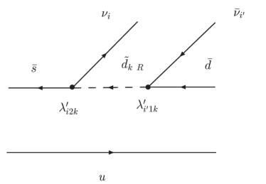
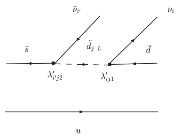
Figure 1: R-parity violating diagrams contributing to the process $K^{+}\to\pi^{+}\nu{\bar{\nu}}$.

Including the R-parity violating processes, the branching ratio for the rare decay $K^{+}\to\pi^{+}\nu\bar{\nu}$ can be written in the following form:

$$BR(K^{+}\to\pi^{+}\nu\bar{\nu})=\frac{\bar{\kappa}_{+}}{3\lambda^{2}}\left(\sum_{l}\mid C_{l}^{\mathrm{model}}+\frac{\epsilon_{ll}}{4k\,(200\;\mathrm{GeV})^{2}}\mid^{2}+\sum_{b\not=l}\frac{\mid\epsilon_{bl}\mid^{2}}{16k^{2}\,(200\;\mathrm{GeV})^{4}}\right)$$ (23)

Throughout our analysis we assume $C_{l}^{\mathrm{model}}$ to be either $C_{l}^{SM}=\lambda_{c}X_{c}^{l}+\lambda_{t}\,X_{t}$ or $C_{l}^{SUSY}=\lambda_{c}X_{c}^{l}+\lambda_{t}\,X_{\mathit{new}}$. The factor “$k$” is given by

$$k=\frac{G_{f}\alpha(m_{Z})}{\sqrt{2}\pi\sin^{2}(\theta_{w})}=8.88\times 10^{-8}\ \mathrm{GeV}^{-2}$$ (24)

Errors are below 1% and are therefore negligible compared to other errors. The R-parity violating couplings are contained in the $\epsilon_{ij}$ which are defined as

$$\epsilon_{ij}=\sum_{n}\left(\frac{\lambda_{i2n}^{{}^{\prime}*}\lambda_{j1n}^{{}^{\prime}}}{m_{\tilde{d}n_{R}}^{2}}-\frac{\lambda_{in1}^{{}^{\prime}*}\lambda_{jn2}^{{}^{\prime}}}{m_{\tilde{d}n_{L}}^{2}}\right)(200\;\mathrm{GeV})^{2}\;.$$ (25)

Note that we give our constraints for degenerate squarks masses of 200 GeV as the recent lower bounds on squarks have increased [16]. $\lambda^{\prime}_{ijk}$ are complex parameters such that the phase of $\epsilon_{ij}$ is a priori not known.

In contrast to the standard model and the SUSY contributions, R-parity violating couplings can induce processes with a neutrino and an antineutrino of different flavour in the final state. This leads to the last term in Eq. 23. Obviously no interferences occur with the standard model/SUSY contribution in that case. The R-parity violating processes with the same neutrino flavour in the final state, however, interfere with the SM/SUSY contribution as can be seen from the first term in Eq. 23. The resulting contribution to the branching ratio is:

$$BR^{Int}=-2\frac{\bar{\kappa}_{+}}{12\lambda^{2}\;k(200\;\mathrm{GeV})^{2}}\sum_{l}Re(C_{l}^{model}\;\epsilon_{ll})$$ (26)

5 Full analysis and constraints on the $\lambda^{\prime}$

Within this section we will discuss different bounds on the $\lambda^{\prime}_{ijk}$ arising from the process $K^{+}\to\pi^{+}\nu\bar{\nu}$. Of course it is not possible to establish bounds on each of the 27 couplings separately. Under some assumption it is possible to constrain certain combinations of couplings. We will perform our analysis in three steps. First we will neglect all contributions except the tree level R-parity violating ones in order to estimate their order of magnitude in comparison with the SM and SUSY contributions. The “pure” R-parity violating branching ratio is given by

$$BR^{R_{p}}=\frac{\bar{\kappa}_{+}}{48\lambda^{2}\;k^{2}(200\;\mathrm{GeV})^{4}}\sum_{i,j}\mid\epsilon_{ij}\mid^{2}~{}.$$ (27)

Comparing this with the experimental value it is therefore straightforward to derive an upper bound for the sum of all $\epsilon_{ij}$:

$$\sum_{i,j}\mid\epsilon_{ij}\mid^{2}<5.6\times 10^{-10}\;.$$ (28)

With squarks at $100$ GeV, we have $\sum_{i,j}\mid\epsilon_{ij}\mid^{2}<0.35\times 10^{-10}$. This bound is much lower than the upper bounds $2.3\times 10^{-9}$ and $2.3\times 10^{-10}$ obtained respectively by Choudhoury and Roy [29] a few years ago and recently by the authors of Ref. [26], both using degenerate squarks masses of $100$ GeV. On the one hand this shows how much data on $K^{+}\to\pi^{+}\nu{\bar{\nu}}$ has improved recently, but on the other hand this implies that the one-loop SM or SUSY contributions should be properly taken into account in order to obtain a realistic limit as they are of the same order as the possible R-parity violating tree-level ones.

From our previous discussion, we have drawn the conclusion that SUSY has to be included in the analysis of $K^{+}\to\pi^{+}\nu\bar{\nu}$. In the next step we will therefore include the SUSY contribution. Note that this contains the standard model contribution as a special case ($r_{K}=1$ and $\theta_{K}=0$). We will therefore not discuss the latter separately. An analysis of the resulting bounds including only the SM contribution has recently been performed for some special cases in Ref. [30].

Since we aim to obtain an upper-bound on the R-parity violating couplings, we assume the SUSY contribution (which already includes SM) to be minimal (corresponding to $r_{K}=0.5$ and $\theta_{K}=25^{o}$) in order to allow for the largest possible contribution from R-parity violating terms. To simplify the discussion we will, for the time being, neglect interferences (cf. section 4). The upper bound for the sum of the $\epsilon_{ij}$ can then slightly be improved compared to the case without any SUSY contribution given in Eq. 28. We obtain

$$\sum_{i,j}\mid\epsilon_{ij}\mid^{2}<4.45\times 10^{-10}~{}.$$ (29)

This limit can be translated to an upper bound on the product of two couplings by naively setting all the couplings to zero except one product. This procedure results in the following bounds:

$$\mid\frac{\lambda_{i2n}^{{}^{\prime}*}\lambda_{j1n}^{{}^{\prime}}}{m_{\tilde{d}n_{R}}^{2}}\mid\ <2.11\times 10^{-5}$$ (30)

$$\mid\frac{\lambda_{in1}^{{}^{\prime}*}\lambda_{jn2}^{{}^{\prime}}}{m_{\tilde{d}n_{L}}^{2}}\mid\ <2.11\times 10^{-5}$$ (31)

Of course, more realistic and precise constraints should take into account interferences. This, however, makes the extraction of upper bounds harder and no simple bounds in the sense of Eqs. 29, 30, 31 can be given. In the following part we will assume that only final states with the same neutrino flavour occur. Thus only $\epsilon_{ij}$ with $i=j$ has to be taken into account. The general equation verified by the $\epsilon_{ii}$ can be written in the following way:

$$\sum_{i=e,\mu,\tau}\left(Re(\epsilon_{ii})+\frac{\alpha_{i}}{2}\right)^{2}\;+\sum_{i=e,\mu,\tau}\left(Im(\epsilon_{ii})+\frac{\beta}{2}\right)^{2}=R^{2}\;,$$ (32)

Taking only one of the $\epsilon_{ii}$ nonzero, this equation describes a circle in the complex plane, whose parameters are listed in Table 1 for the case of the standard model ($r_{K}=1$ and $\theta_{K}=0$) and for the “minimal” SUSY contribution, corresponding to $r_{K}=0.5$ and $\theta_{K}=25^{o}$. The radius R contains the term $\displaystyle\frac{48\lambda^{2}\;k^{2}}{\bar{\kappa}_{+}(200\;\mathrm{GeV})^{-4}}(BR^{exp}-BR^{th})$ and the shifts $\alpha$ and $\beta$. The shifts depends on the CKM inputs and on the loop-functions $X_{t}$ and $X_{c}^{l}$. The $c_{i}$’s are the corrections of $\alpha$ due to the implicit dependence on the lepton masses $m_{i}$.

The resulting constraints in the complex plane on $\epsilon_{11}$ are displayed in Fig. 2. Constraints on $\epsilon_{22}$ and $\epsilon_{33}$ can be obtained in the same way and are of the same order of magnitude. To have an idea of the influence of the interferences, we may choose the point of coordinates (Re($\epsilon_{11}$)=-2, Im($\epsilon_{11}$)=-2) on the SUSY circle of Fig.2. It is approximately the point which gives the maximum value for $\mid\epsilon_{11}\mid$. We have $\mid\epsilon_{11}\mid=2.8\times 10^{-5}$ and then we deduce, in the same manner, limits on products of RPV couplings:

$$\mid\frac{\lambda_{i2n}^{{}^{\prime}*}\lambda_{i1n}^{{}^{\prime}}}{m_{\tilde{d}n_{R}}^{2}}\mid\ \mathrel{\raise 1.29167pt\hbox{$<$\kern-7.5pt\lower 4.30554pt\hbox{$\sim$}}}2.8\times 10^{-5}$$ (33)

$$\mid\frac{\lambda_{in1}^{{}^{\prime}*}\lambda_{in2}^{{}^{\prime}}}{m_{\tilde{d}n_{L}}^{2}}\mid\ \mathrel{\raise 1.29167pt\hbox{$<$\kern-7.5pt\lower 4.30554pt\hbox{$\sim$}}}2.8\times 10^{-5}$$ (34)

These are 30$\%$ bigger than the ones in Eqs. 30, 31 and so this numerical example shows that interferences may have a significant influence.

	$\alpha_{i}$	$c_{e}=c_{\mu}$	$c_{\tau}$	$\beta$	$R^{2}$
SM	$c_{i}\,(2.03\times 10^{-5})$	1	0.89	$5.79\times 10^{-6}$	$2.48\times 10^{-10}\,+\sum_{i}\alpha_{i}^{2}/4\,+\beta^{2}/4$
SUSYmin	$c_{i}\,(1.17\times 10^{-5})$	1	0.81	$5.49\times 10^{-6}$	$4.47\times 10^{-10}\,+\sum_{i}\alpha_{i}^{2}/4\,+\beta^{2}/4$

Table 1: Values of the constants appearing in Eq. 32

Figure 2: Allowed region for $Re(\epsilon_{11})$ and $Im(\epsilon_{11})$ in units of $10^{-5}$. In order to compare with the very recent constraints on these R-parity violating couplings [30], remember that we take 200 GeV as reference value for the mass of the squarks.

6 Conclusions

We have investigated the decay $K^{+}\to\pi^{+}\nu{\bar{\nu}}$ and related rare decays as a probe of physics beyond the standard model. As a starting point we have obtained the standard model value using updated experimental values for all the relevant parameters. We found a slightly bigger branching than other recent estimates: $B=(8.18\pm 1.22)\times 10^{-11}$. Furthermore we have analyzed the supersymmetric contributions in the mass-insertion approximation and corrected a minor misprint in the neutralino contribution that was present in the existing literature. The main concern of this paper was to obtain stringent limits on the R-parity violating couplings. Assuming that the process $K^{+}\to\pi^{+}\nu{\bar{\nu}}$ is governed entirely by RPV processes, the bounds on RPV couplings can be lowered with respect to previous analysis (cf. Refs. [29, 26]) due to recent data. Recent experimental limits, however, indicate that SM and SUSY contributions, which can give up to 50% of the SM one, should be taken into account in order to establish limits on the RPV couplings. We performed an analysis including all these effects and we have shown that interferences can have an effect of the order of 30 % on the bounds on RPV couplings.

Appendix A Explicit expressions of the supersymmetric contributions

We only list the final formulae, more details and explanations (on the basis of the fermions and sfermions fields, Feynman graphs) can be found in Refs. [9, 10]. The misprints of [9] have been corrected and functions are written in the notation of [10]. We based our calculations on [32, 33].

General notations :

• $x_{ij}$ denote ratios of squared masses (for example : $\displaystyle x_{i\tilde{t}_{R}}=\frac{M_{\tilde{C}_{i}}^{2}}{M_{\tilde{t}_{R}}^{2}}$),

• ${\bf j}(x_{1},..,x_{n})$ and ${\bf k}(x_{1},..,x_{n})$ are the loop functions defined in [9] (singularities of these functions in the case of equal arguments become derivatives).

Charged Higgses contribution

$$X_{H^{\pm}}=X_{H^{\pm}}(x_{H}=\frac{M_{W}^{2}}{m_{H^{\pm}}^{2}})=\frac{m_{t}^{2}}{8M_{W}^{2}tan^{2}\beta}x_{H}\left(\frac{1}{(x_{H}-1)}-\frac{\ln(x_{H})}{(x_{H}-1)^{2}}\right)$$ (35)

Chargino contributions

• $\displaystyle g_{t}=\frac{m_{t}}{\sqrt{2}M_{W}\sin\beta}$ is the top-quark coupling,

• U and V are 2x2 unitary matrices that diagonalize the chargino mass matrix:

  $$M_{\tilde{C}}=U^{T}\,diag(M_{\tilde{C}_{1}},M_{\tilde{C}_{2}})\,V,\ M_{\tilde{C}_{i}}>0$$ (36)

  $$M_{\tilde{C}}=\left(\begin{array}[]{cc}M_{2}&\sqrt{2}M_{W}\sin\beta\\ \sqrt{2}M_{W}\cos\beta&\mu\end{array}\right)$$ (37)

  They can be found in explicit form in [34] [35].

1-RR contribution

$$C^{0}_{RR}=\sum_{i;j=1,2}\left((C^{0})^{Pen}_{ij}+\ (C^{0})^{Box}_{ij}\right)$$ (38)

$$(C^{0})^{Pen}_{ij}=\frac{g_{t}^{2}}{8}\,V_{2j}^{{\dagger}}V_{i2}\left({\bf k}(x_{i\tilde{t}_{R}},x_{j\tilde{t}R})\,V_{j1}V_{1i}^{{\dagger}}-2\,{\bf j}(x_{i\tilde{t}_{R}},x_{j\tilde{t}_{R}})\sqrt{x_{i\tilde{t}_{R}}\,x_{j\tilde{t}_{R}}}\,U_{i1}U_{1j}^{{\dagger}}\right)\;$$ (39)

$$(C^{0})^{Box}_{ij}=\frac{g_{t}^{2}}{2}\,x_{W\tilde{t}_{R}}\,{\bf j}(x_{i\tilde{t}_{R}},x_{j\tilde{t}_{R}},x_{\tilde{e}_{L}\tilde{t}_{R}})\,V_{2j}^{{\dagger}}V_{i2}U_{i1}U_{1j}^{{\dagger}}$$ (40)

2-LL contribution

$$C_{LL}=\sum_{i;j=1,2}\left((C_{LL})^{Pen}_{ij}+\ (C_{LL})^{Box}_{ij}\right)$$ (41)

$$(C_{LL})^{Pen}_{ij} = -\frac{1}{8}\,V_{1j}^{{\dagger}}V_{i1}\left({\bf k}(x_{i\tilde{u}_{L}},x_{j\tilde{u}_{L}},1)\,V_{j2}V_{2i}^{{\dagger}}-2\,{\bf j}(x_{i\tilde{u}_{L}},x_{j\tilde{u}_{L}},1)\sqrt{x_{i\tilde{u}_{L}}\,x_{j\tilde{u}_{L}}}U_{i2}U_{2j}^{{\dagger}}\right)$$

$$(C_{LL})^{Box}_{ij} = \frac{1}{2}\,x_{W\tilde{u}_{L}}\,{\bf j}(x_{i\tilde{u}_{L}},x_{j\tilde{u}_{L}},x_{\tilde{e}_{L}\tilde{u}_{L}},1)\,V_{1j}^{{\dagger}}V_{i1}U_{i1}U_{1j}^{{\dagger}}$$ (43)

3-LR and RL contribution

$$C_{LR}=\sum_{i;j=1,2}\left((C_{LR})^{Pen}_{ij}+\ (C_{LR})^{Box}_{ij}\right)$$ (44)

$$C_{RL}=\sum_{i;j=1,2}\left((C_{RL})^{Pen}_{ij}+\ (C_{RL})^{Box}_{ij}\right)$$ (45)

$$(C_{LR})^{Pen}_{ij} = -\frac{m_{t}g_{t}}{8m_{\tilde{u}_{L}}}\,V_{2j}^{{\dagger}}V_{i1}\times$$

$$\left({\bf k}(x_{i\tilde{u}_{L}},x_{j\tilde{u}_{L}},x_{\tilde{t}_{R}\tilde{u}_{L}})V_{j1}V_{1i}^{{\dagger}}-{\bf k}(x_{i\tilde{u}_{L}},x_{\tilde{t}_{R}\tilde{u}_{L}},1)\delta_{ij}\right.$$

$$\left.-2\,{\bf j}(x_{i\tilde{u}_{L}},x_{j\tilde{u}_{L}},x_{\tilde{t}_{R}\tilde{u}_{L}})U_{i1}U_{1j}^{{\dagger}}\sqrt{x_{i\tilde{u}_{L}}\,x_{j\tilde{u}_{L}}}\right)$$

$$(C_{LR})^{Box}_{ij} = -\frac{m_{t}g_{t}}{2m_{\tilde{u}_{L}}}\,x_{W\tilde{u}_{L}}\,{\bf j}(x_{i\tilde{u}_{L}},x_{j\tilde{u}_{L}},x_{\tilde{t}_{R}\tilde{u}_{L}},x_{\tilde{e}_{L}\tilde{u}_{L}})\,V_{2j}^{{\dagger}}V_{i1}U_{i1}U_{1j}^{{\dagger}}$$ (47)

$$(C_{RL})^{Pen}_{ij} = -\frac{m_{t}g_{t}}{8m_{\tilde{u}_{L}}}\,V_{1j}^{{\dagger}}V_{i2}\times$$

$$\left({\bf k}(x_{i\tilde{u}_{L}},x_{j\tilde{u}_{L}},x_{\tilde{t}_{R}\tilde{u}_{L}})\,V_{j2}V_{2i}^{{\dagger}}-{\bf k}(x_{i\tilde{u}_{L}},x_{\tilde{t}_{R}\tilde{u}_{L}},1)\delta_{ij}\right.$$

$$\left.-2\,{\bf j}(x_{i\tilde{u}_{L}},x_{j\tilde{u}_{L}},x_{\tilde{t}_{R}\tilde{u}_{L}})U_{i2}U_{2j}^{{\dagger}}\sqrt{x_{i\tilde{u}_{L}}\,x_{j\tilde{u}_{L}}}\right)$$

$$(C_{RL})^{Box}_{ij} = -\frac{m_{t}g_{t}}{2m_{\tilde{u}_{L}}}\,x_{W\tilde{u}_{L}}\,{\bf j}(x_{i\tilde{u}_{L}},x_{j\tilde{u}_{L}},x_{\tilde{t}_{R}\tilde{u}_{L}},x_{\tilde{e}_{L}\tilde{u}_{L}})V_{1j}^{{\dagger}}V_{i2}U_{i2}U_{2j}^{{\dagger}}$$ (49)

Neutralino contribution

The neutralino contribution is potentially large since $R^{D}_{s_{L}d_{L}}$ can be large such that it should be taken into account. Compared to Ref. [9], we corrected a minus sign in front of the function k in expression for the penguin diagram. An overall missing factor (-1/2) has been corrected too. The first two diagrams in figure 7 in Ref. [9] involving a squark-squark-$Z$ vertex are cancelled by self-energy corrections. The two other contributions give:

$$\tilde{N}=\sum_{n;m=1..4}\left((\tilde{N})^{Pen}_{nm}+\ (\tilde{N})^{Box}_{nm}\right)$$ (50)

$$(\tilde{N})_{nm}^{Pen} = -\frac{1}{2}\,{\bf j}(x_{n\tilde{d}_{L}},x_{m\tilde{d}_{L}},1)\sqrt{x_{n\tilde{d}_{L}}\,x_{m\tilde{d}_{L}}}\,W^{T}_{n}(d_{L})[W_{n4}W_{4m}^{{\dagger}}-W_{n3}W_{3m}^{{\dagger}}]W^{*}_{m}(d_{L})$$ (51)

$$\ \ -\frac{1}{4}\,{\bf k}(x_{n\tilde{d}_{L}},x_{m\tilde{d}_{L}},1)\,W^{T}_{n}(d_{L})[W^{*}_{n4}W_{4m}^{T}-W_{n3}^{*}W_{3m}^{T}]W^{*}_{m}(d_{L})$$

$$(\tilde{N})_{nm}^{Box} = x_{W\tilde{d}_{L}}\{{\bf k}(x_{n\tilde{d}_{L}},x_{m\tilde{d}_{L}},x_{\tilde{\nu}_{L}\tilde{d}_{L}},1)\,W^{T}_{n}(d_{L})W^{*}_{n}(\nu_{L})W^{T}_{m}(\nu_{L})W^{*}_{m}(d_{L})$$

$$\ \ +\,2\,{\bf j}(x_{n\tilde{d}_{L}},x_{m\tilde{d}_{L}},x_{\tilde{\nu}_{L}\tilde{d}_{L}},1)\sqrt{x_{n\tilde{d}_{L}}\,x_{m\tilde{d}_{L}}}\,W^{T}_{n}(d_{L})W_{n}(\nu_{L})W^{{\dagger}}_{m}(\nu_{L})W^{*}_{m}(d_{L})\}$$

W is the unitary matrix which diagonalizes the Neutralino mass matrix :

$$M_{\tilde{N}}=W^{T}.diag(M_{\tilde{N}_{1}},M_{\tilde{N}_{2}},M_{\tilde{N}_{3}},M_{\tilde{N}_{4}}).W\ \ \,,M_{\tilde{N}_{n}}>0$$ (53)

$$M_{\tilde{N}}=\left(\begin{array}[]{cccc}M_{1}&0&-M_{Z}\sin\Theta_{W}\cos\beta&M_{Z}\sin\Theta_{W}\sin\beta\\ 0&M_{2}&M_{Z}\cos\Theta_{W}\cos\beta&-M_{Z}\cos\Theta_{W}\sin\beta\\ -M_{Z}\sin\Theta_{W}\cos\beta&M_{Z}\cos\Theta_{W}\cos\beta&0&-\mu\\ M_{Z}\sin\Theta_{W}\sin\beta&-M_{Z}\cos\Theta_{W}\sin\beta&-\mu&0\end{array}\right)$$

By $W_{n}(x)$ we denote $T_{3}(x)\,W_{n2}+\tan\theta_{W}\,\frac{Y(x)}{2}\,W_{n1}$, where $T_{3}(x)$ is the third component of the weak isospin and $Y(x)$ the hypercharge.

References

• [1] M. Ciuchini et al., JHEP 0107 (2001) 013 [arXiv:hep-ph/0012308]; A. Stocchi, arXiv:hep-ph/0405038; A. Stocchi, private communication for the values with the most recent top quark mass; see also www.utfit.org for details on the CKM fit.
• [2] P. Azzi et al. [CDF Collaboration], arXiv:hep-ex/0404010.
• [3] S. C. Adler et al. [E787 Collaboration], Phys. Rev. Lett.  79 (1997) 2204 [arXiv:hep-ex/9708031]; S. Adler et al. [E787 Collaboration], arXiv:hep-ex/0403034; V. V. Anisimovsky et al. [E949 Collaboration], arXiv:hep-ex/0403036.
• [4] A. Sher et al., Phys. Rev. Lett. 91 (2003) 261802; AIP Conf. Proc.  698 (2004) 381 [arXiv:hep-ex/0305042].
• [5] G. Buchalla, A. J. Buras and M. E. Lautenbacher, Rev. Mod. Phys.  68 (1996) 1125 [arXiv:hep-ph/9512380].
• [6] S. Bertolini and A. Masiero, Phys. Lett. B 174 (1986) 343; G. F. Giudice, Z. Phys. C 34 (1987) 57; S. Bertolini, F. Borzumati, A. Masiero and G. Ridolfi, Nucl. Phys. B 353 (1991) 591; I. I. Y. Bigi and F. Gabbiani, Nucl. Phys. B 367 (1991) 3; A. J. Buras, M. E. Lautenbacher and G. Ostermaier, Phys. Rev. D 50 (1994) 3433 [arXiv:hep-ph/9403384]; G. Couture and H. König, Z. Phys. C 69 (1995) 167 [arXiv:hep-ph/9503299]; Y. Nir and M. P. Worah, Phys. Lett. B 423 (1998) 319 [arXiv:hep-ph/9711215].
• [7] G. Buchalla and A. J. Buras, Nucl. Phys. B 548 (1999) 309 [arXiv:hep-ph/9901288].
• [8] G. D’Ambrosio and G. Isidori, Phys. Lett. B 530 (2002) 108 [arXiv:hep-ph/0112135].
• [9] A. J. Buras, A. Romanino and L. Silvestrini, Nucl. Phys. B 520 (1998) 3 [arXiv:hep-ph/9712398].
• [10] G. Colangelo and G. Isidori, JHEP 9809 (1998) 009 [arXiv:hep-ph/9808487].
• [11] N. Cabibbo, Phys. Rev. Lett.  10 (1963) 531; M. Kobayashi and T. Maskawa, Prog. Theor. Phys.  49 (1973) 652.
• [12] G. Buchalla and A. J. Buras, Nucl. Phys. B 398 (1993) 285; G. Buchalla and A. J. Buras, Nucl. Phys. B 400 (1993) 225; G. Buchalla and A. J. Buras, Nucl. Phys. B 412 (1994) 106 [arXiv:hep-ph/9308272]; M. Misiak and J. Urban, Phys. Lett. B 451 (1999) 161 [arXiv:hep-ph/9901278].
• [13] G. Buchalla and G. Isidori, Phys. Lett. B 440, 170 (1998) [arXiv:hep-ph/9806501]; A. F. Falk, A. Lewandowski and A. A. Petrov, Phys. Lett. B 505, 107 (2001) [arXiv:hep-ph/0012099]; G. Buchalla and A. J. Buras, Phys. Rev. D 57, 216 (1998) [arXiv:hep-ph/9707243].
• [14] W. J. Marciano and Z. Parsa, Phys. Rev. D 53 (1996) 1.
• [15] L. Wolfenstein, Phys. Rev. Lett.  51 (1983) 1945.
• [16] S. Eidelman et al, Phys. Lett. B592, 1 (2004) and pdg.lbl.gov.
• [17] Y. Kiyo and Y. Sumino, Phys. Rev. D 67 (2003) 071501 [arXiv:hep-ph/0211299].
• [18] A. J. Buras, F. Schwab and S. Uhlig, arXiv:hep-ph/0405132.
• [19] G. Buchalla, G. D’Ambrosio and G. Isidori, Nucl. Phys. B 672 (2003) 387 [arXiv:hep-ph/0308008].
• [20] G. Isidori, C. Smith and R. Unterdorfer, arXiv:hep-ph/0404127.
• [21] A. Alavi-Harati et al. [The E799-II/KTeV Collaboration], Phys. Rev. D 61 (2000) 072006 [arXiv:hep-ex/9907014].
• [22] S. Dimopoulos and H. Georgi, Nucl. Phys. B 193 (1981) 150; J. R. Ellis and D. V. Nanopoulos, Phys. Lett. B 110 (1982) 44; R. Barbieri and R. Gatto, Phys. Lett. B 110 (1982) 211; M. J. Duncan, Nucl. Phys. B 221 (1983) 285; J. F. Donoghue, H. P. Nilles and D. Wyler, Phys. Lett. B 128 (1983) 55.
• [23] L. J. Hall, V. A. Kostelecky and S. Raby, Nucl. Phys. B 267 (1986) 415.
• [24] F. Gabbiani, E. Gabrielli, A. Masiero and L. Silvestrini, Nucl. Phys. B 477 (1996) 321 [arXiv:hep-ph/9604387]; M. Misiak, S. Pokorski and J. Rosiek, Adv. Ser. Direct. High Energy Phys.  15 (1998) 795 [arXiv:hep-ph/9703442].
• [25] S. Davidson and J. R. Ellis, Phys. Rev. D 56 (1997) 4182 [arXiv:hep-ph/9702247]; S. Davidson and J. R. Ellis, Phys. Lett. B 390 (1997) 210 [arXiv:hep-ph/9609451]; S. Davidson, Phys. Lett. B 439 (1998) 63 [arXiv:hep-ph/9808425].
• [26] R. Barbier et al., arXiv:hep-ph/0406039 and references therein.
• [27] Y. Grossman, G. Isidori and H. Murayama, Phys. Lett. B 588 (2004) 74 [arXiv:hep-ph/0311353].
• [28] K. Agashe and M. Graesser, Phys. Rev. D 54 (1996) 4445 [arXiv:hep-ph/9510439].
• [29] D. Choudhury and P. Roy, Phys. Lett. B 378 (1996) 153 [arXiv:hep-ph/9603363].
• [30] N. G. Deshpande, D. K. Ghosh and X. G. He, arXiv:hep-ph/0407021.
• [31] D. Binosi and L. Theussl, Comput. Phys. Commun.  161 (2004) 76 [arXiv:hep-ph/0309015].
• [32] H. E. Haber and G. L. Kane, Phys. Rept.  117 (1985) 75.
• [33] T. Inami and C. S. Lim, Prog. Theor. Phys.  65 (1981) 297 [Erratum-ibid.  65 (1981) 1772].
• [34] J. L. Kneur and G. Moultaka, Phys. Rev. D 61 (2000) 095003 [arXiv:hep-ph/9907360].
• [35] K. Cankocak, A. Aydemir and R. Sever, Phys. Rev. D 69 (2004) 075010 [arXiv:hep-ph/0402169].