Two- and three-body color flux tubes in the
Chromo Dielectric Model

Abstract

Using the framework of the Chromo Dielectric Model we perform an analysis of color electric flux tubes in meson-like $q\bar{q}$ and baryon-like $qqq$ quark configurations. We discuss the Abelian color structure of the model and point out a symmetry in color space as a remnant of the SU(3) symmetry of QCD. The generic features of the model are discussed by varying the model parameters. We fix these parameters by reproducing the string tension $\tau=980\,$MeV/fm and the transverse width $\rho=0.35\,$fm of the $q\bar{q}$ flux tube obtained in lattice calculations. We use a bag constant $B^{1/4}=(240-260)\,$MeV, a glueball mass $m_{g}=(1000-1700)\,$MeV and a strong coupling constant $C_{F}\alpha_{s}=0.2-0.3$. We show that the asymptotic string profile of an infinitely long flux tube is already reached for $q\bar{q}$ separations $R\geq 1.0\,$fm. A connection to the Dual Color Superconductor is made by extracting a magnetic current from the model equations and a qualitative agreement between the two descriptions of confinement is shown. In the study of the $qqq$ system we observe a $\mathsf{\Delta}$-like geometry for the color electric fields and a Y-like geometry in the scalar fields both in the energy density distribution and in the corresponding potentials. The resulting total $qqq$ potential is described neither by the $\mathsf{\Delta}$-picture nor by the Y-picture alone.

I Introduction

The structure of hadrons is still a subject of discussion. It is widely accepted that Quantum Chromodynamics (QCD) is the right theory for strong interactions, and that the properties of hadrons can be described within this framework. QCD has been tested successfully in the region of large momentum transfer, where perturbative methods work due to asymptotic freedom. However, in the region of small relative momentum, where the formation of hadrons sets in and confinement plays a dominant role, a calculation from first principles is still limited to lattice techniques.

In order to understand the formation of hadrons out of quarks and gluons dynamically, and in turn the interactions of hadrons with each other, one still has to rely on models that include the phenomenon of confinement. Such phenomenological models are for example the bag model Chodos et al. (1974a, b), where quarks are treated as free particles restricted to predefined bags, the quark molecular dynamics model Hofmann et al. (2000); Scherer et al. (2001), where colored quarks obey the classical Hamilton dynamics bound by a linear confining potential, or the model of the dual superconductor Baker et al. (1991); Ripka (2004), where confinement is achieved by monopole condensation ’t Hooft (1974); Polyakov (1974) and an accompanying dual supercurrent. The model of the stochastic vacuum relies on the calculation of Wilson-loops in a Gaussian approximation Dosch (1987); Shoshi et al. (2003) which leads to a linear potential between quarks and anti-quarks.

In this work we adopt the Chromo Dielectric Model (CDM) Friedberg and Lee (1977a, b); Wilets (1989), which is an extension of the bag model in the sense that bags are formed dynamically in the presence of quarks. Mack Mack (1984) and Pirner et al. Pirner et al. (1984); Mathiot et al. (1989); Pirner (1992) have given a renormalization group derivation of the lattice colordielectric model, which also has a scalar field modelling confinement, but keeps strongly coupled non-Abelian fields in the large distance action. A Monte-Carlo calculation within the lattice colordielectric model was done in Pirner et al. (1987); Grossmann et al. (1991). The model has already been used to calculate hadron properties like low lying baryon masses, the nucleon magnetic moments and the (axial-vector)/vector coupling constant ratio Goldflam and Wilets (1982) and nucleon–nucleon interactions in vacuum and in nuclear matter Pirner et al. (1984); Achtzehnter et al. (1985). Schuh et al. (1986); Koepf et al. (1994); Pepin et al. (1996). In another approach the description has been used within a transport theoretical scheme to describe the dynamics Vetter et al. (1995); Kalmbach et al. (1993); Loh et al. (1997) of quarks bound in nucleons and strings. In Traxler et al. (1999) a full molecular dynamics simulation for colored quarks was performed, showing the ability of the model to produce color neutral hadrons out of a gas of colored quarks, thus giving for the first time a microscopic description of hadronization from a quark gluon plasma.

The parameters used in Vetter et al. (1995); Kalmbach et al. (1993); Loh et al. (1997); Traxler et al. (1999), which define the model, were mostly motivated by phenomenological arguments and not subject to a further investigation. The resulting color flux tubes are rather large objects with a string radius up to 1 fm. In addition the linear rising $q\bar{q}$ potential was only seen for quark separations $R>1\,$fm. On the other hand, lattice calculations Bali et al. (1995); Trottier and Woloshyn (1993) indicate, that the radius of a colored flux tube is much smaller than 1 fm, and that the $q\bar{q}$ potential already develops a linear rising term for separations larger than $R=0.2\,$fm. In addition, on the lattice a clear Coulomb-like potential was observed for quark separations $R<0.2\,$fm, which has not been resolved in Traxler et al. (1999). In the present work we model the results from lattice calculations as well as possible within the framework of the CDM. On the lattice the most accurate results were obtained in SU(2) Bali et al. (1995). We assume that the shape of the color flux tube does not depend significantly on the underlying Lie algebra. Therefore we compare the results of our calculations to those obtained in lattice SU(2) theory. The quantities that we want to reproduce are the transverse shape of a flux tube of given length, and the linear coefficient of the $q\bar{q}$ potential obtained in meson spectroscopy Eichten et al. (1975); Quigg and Rosner (1979); Eichten et al. (1980).

Having established a set of parameters matching the criteria above, we then analyze the structure of the flux tubes. The emphasis will be on the question how the string is build up when the constituents of the string are separated from each other. In varying the $q\bar{q}$ distance $R$ we probe both the perturbative (small $R$) and the non-perturbative region (large $R$). We will also see how fast the transition from one to the other sets in and from which distances on the string picture holds.

The formation of strings is not restricted to $q\bar{q}$ objects. In QCD one has the possibility to build up color neutral objects from three quarks. When the pairwise quark separations are large compared to the characteristic width of the string, color flux tubes will stretch between the quarks. In general two geometrically different pictures are possible. The first is the so called Y-geometry, where three flux tubes meet at a central point Artru (1975); Brambilla et al. (1994). The second one is the $\mathsf{\Delta}$-geometry, where the three quarks are connected pairwise Cornwall (1977, 1996). The three-quark potential emerging from these two pictures has been compared to lattice results in Alexandrou et al. (2002a) and Takahashi et al. (2002). Due to the lack of numerical precision the two groups obtained different results. Therefore lattice calculations cannot clearly rule out one of the pictures so far. Within our model we are able to describe those baryonic quark configurations not only on the level of the $qqq$ potential but also on the level of the energy distributions. We can study the structure of the formed flux tubes and discriminate between the two geometries.

The main goal of this work is to fix the model parameters on lattice data of $q\bar{q}$ flux tubes. The parameters obtained will be used to describe both the shape and the potential of the three quark system within CDM. The structure of this work is as follows. In section II we present the model and its specific mechanism of confinement. In section III we analyze the dependence of the shape and the potential of a $q\bar{q}$ string on the variation of the parameters introduced in the model. We compare our numerical $q\bar{q}$ results for three specific sets of parameters to those obtained within lattice gauge calculations in section IV and extend the analysis to baryon-like three-quark systems in section V. In the appendix A we give a description of the algorithm used in our numerical calculations.

II The Chromo dielectric Model

Presumably the non-Abelian gluon interactions of QCD are responsible for a highly structured non-perturbative vacuum. Although it is difficult to disentangle these interactions from first principles, the large scale behavior of strong interactions might be simple. In the Chromo Dielectric Model (CDM) one assumes, that the QCD vacuum behaves as a perfect dielectric medium, i.e. as a medium with vanishing dielectric constant. Colored quarks embedded in this vacuum produce electric color fields. In the presence of the dielectric medium these fiels are compressed in well defined flux tubes connecting quarks with opposite charge.

To be more specific, the medium is described by a colorless scalar field $\sigma$ which mediates the vacuum properties via the dielectric function $\kappa(\sigma)$. The confinement field itself is evolving in the presence of a scalar self interaction $U(\sigma)$.

As the dynamics and the non-Abelian interactions of the gluon sector are merged in the confinement field $\sigma$ and its dielectric coupling $\kappa(\sigma)$ one is left with a set of two Abelian gluon fields $A^{\mu,a}$ that interacts with the dielectric medium. In principle it is possible to formulate the model with dynamical quarks, described by a Dirac-like Lagrangian Goldflam and Wilets (1982); Schuh et al. (1986); Fai et al. (1988), but in this work we concentrate on the structure of color flux tubes. Therefore we treat the quarks as external sources of color fields. The CDM can now be defined by the following Lagrange density:

$${\cal L} = {\cal L}_{g}+{\cal L}_{\sigma}\quad,$$ (1a)

$${\cal L}_{g} = -{\textstyle\frac{1}{4}}{\kappa(\sigma)}F_{\mu\nu}^{a}F^{\mu\nu,{a}}-g_{s}\;j_{\mu}^{a}\,A^{\mu,a}\quad,$$ (1b)

$${\cal L}_{\sigma} = {{\textstyle\frac{1}{2}}\partial_{\mu}\sigma\partial^{\mu}\sigma-U(\sigma)}\quad,$$ (1c)

$$F^{\mu\nu,{a}} = \partial^{\mu}A^{\nu,a}-\partial^{\nu}A^{\mu,a},\;\;\;a\in\{3,8\}\quad.$$ (1d)

The color fields $A^{\mu,a}$ couple to the color charge current $j^{\mu,a}=(\rho^{a},\vec{\jmath}^{a})$ classically with a strong coupling constant $g_{s}$ which we have not included in the definition of the current. The charge density is defined as a sum over all charged sources, i.e. the quarks, $\rho^{a}(\vec{x})=\sum_{k}q_{k}^{a}w(\vec{x}-\vec{x}_{k})$, where the $q^{a}$ are the color charges of the quarks. In the static case we are interested in, the spatial part of the color current vanishes $\vec{\jmath}=0$. The quarks are in principle point-like objects but in our numerical analysis described in sec. III we assign a finite Gaussian width $w(\vec{x})=(2\pi r_{0}^{2})^{-3/2}\exp(-\vec{x}^{2}/2r_{0}^{2})$ to each quark. The width is introduced for numerical reasons (see appendix A.1). Throughout this work we adopt a value of $r_{0}=0.02\,$fm, which is large enough to resolve the Gaussian distribution $w(\vec{x})$ and small compared to the dimensions of the flux tubes.

As we are working in an Abelian model inspired by QCD, we have three different colors interacting with only two Abelian color fields. In the color space we choose an arbitrary but fixed base for the quarks in the fundamental representation, $|\mbox{red}\rangle=(1,0,0)^{T}$, $|\mbox{green}\rangle=(0,1,0)^{T}$ and $|\mbox{blue}\rangle=(0,0,1)^{T}$. The color charges $q^{a}$ are then defined as the diagonal entries of the corresponding generators $t^{a}$ of the color group in the same representation $q_{c}^{a}=\langle c|t^{a}|c\rangle$, where $c\in\{\mbox{red (r), green (g), blue (b)}\}$ and $a\in\{3,8\}$. The numerical values of the color charges can be read off from table 1 and are depicted in figure 1. The generators are normalized according to $\operatorname{Tr}\,t^{a}t^{b}=\delta^{ab}/2$. Note that by this definition the $q_{a}$ are reduced by a factor of two as compared to Traxler et al. (1999) and that the strong coupling parameter $g_{s}$ is enhanced by the same factor leaving $g_{s}q_{a}$ fixed.

color	$q^{3}$	$q^{8}$
red	$1/2$	$1/(2\sqrt{3})$
green	$-1/2$	$1/(2\sqrt{3})$
blue	$0$	$-1/\sqrt{3}$

Table 1: The color charges $q^{a}$ of the three colors with respect to the two Abelian color fields.

Figure 1: The color charge $q^{3,8}$ with respect to the color fields $A^{3,8}$.

In the Abelian projected theory one is left with two independent color fields and a remaining U(1)$\times$U(1) gauge symmetry. The corresponding gauge transformations are

$$|c\rangle \rightarrow U(x)|c\rangle=\text{diag}\left(e^{ig_{s}\chi_{1}},e^{ig_{s}\chi_{2}},e^{-ig_{s}(\chi_{1}+\chi_{2})}\right)|c\rangle$$ (2)

$$A^{\mu} \rightarrow \left(A_{a}^{\mu}+\partial^{\mu}\theta_{a}\right)t_{a},$$ (3)

where $\chi_{1}=\tfrac{\theta_{3}}{2}+\tfrac{\theta_{8}}{2\sqrt{3}}$ and $\chi_{2}=-\tfrac{\theta_{3}}{2}+\tfrac{\theta_{8}}{2\sqrt{3}}$. This means that the color charges $q^{3/8}$ are conserved independently and in turn the color fields $F^{\mu\nu,a}$ would be observable fields. However in the Abelian approximation there is a further symmetry, namely a symmetry under special discrete rotations in color space

$$|c\rangle\rightarrow|c^{\prime}\rangle=V|c\rangle\quad.$$ (4)

In matrix form the color rotations are given explicitly as:

$$V_{1}:\quad V_{11}^{1}=\epsilon_{1},\quad V_{22}^{1}=\epsilon_{2},\quad V_{33}^{1} = \epsilon_{1}\epsilon_{2}$$ (5a)

$$V_{2}:\quad V_{12}^{2}=\epsilon_{1},\quad V_{23}^{2}=\epsilon_{2},\quad V_{31}^{2} = \epsilon_{1}\epsilon_{2}$$ (5b)

$$V_{3}:\quad V_{13}^{3}=\epsilon_{1},\quad V_{21}^{3}=\epsilon_{2},\quad V_{32}^{3} = \epsilon_{1}\epsilon_{2}$$ (5c)

$$V_{4}:\quad V_{11}^{4}=\epsilon_{1},\quad V_{23}^{4}=\epsilon_{2},\quad V_{32}^{4} = -\epsilon_{1}\epsilon_{2}$$ (5d)

$$V_{5}:\quad V_{13}^{5}=\epsilon_{1},\quad V_{22}^{5}=\epsilon_{2},\quad V_{31}^{5} = -\epsilon_{1}\epsilon_{2}$$ (5e)

$$V_{6}:\quad V_{12}^{6}=\epsilon_{1},\quad V_{21}^{6}=\epsilon_{2},\quad V_{33}^{6} = -\epsilon_{1}\epsilon_{2},$$ (5f)

where $\epsilon_{1/2}=\pm 1$ and all other matrix elements being zero. There are therefore 4 different copies of each of the $V_{i}$ differing from each other in the signs $\epsilon_{1/2}$. These rotations $V$ act either as a cyclic exchange of all colors $r\rightarrow g\rightarrow b$ (5b) and $b\rightarrow g\rightarrow r$ (5c) or as a pairwise exchange of two colors $g\leftrightarrow b$ (5d), $r\leftrightarrow b$ (5e) and $r\leftrightarrow g$ (5f) with additional phases $\epsilon_{1/2}$. The transformations themselves form a global subgroup $D$ of SU(3), but are not independent from the former U(1)$\times$U(1) gauge group in the sense that out of the set of four copies of $V_{i}$ three of them can be constructed by a combination $V_{i}U(x)$ with $U(x)\in U(1)\times U(1)$. The discrete color rotations $V_{i}$ transform the gauge fields $A^{\mu,3}$ and $A^{\mu,8}$ only into each other without mixing to the non-Abelian gauge fields:

$$A^{\mu}=A^{\mu,3}t_{3}+A^{\mu,8}t_{8}\rightarrow VA^{\mu}V^{\dagger}=A^{\prime\mu,3}t_{3}+A^{\prime\mu,8}t_{8},$$ (6)

with $(A^{\mu,3})^{2}+(A^{\mu,8})^{2}=(A^{\prime\mu,3})^{2}+(A^{\prime\mu,8})^{2}$ and $A^{\prime\mu,a}\neq A^{\mu,a}$. The same is true for the color fields $F^{\mu\nu,3}$ and $F^{\mu\nu,8}$. They are therefore not invariant under the rotations $V\in D$. This is a relict of the full SU(3) gauge symmetry. Of course, the action density (1) and the corresponding energy density, which are the only physical meaningful quantities in the model, are invariant under $V\in D$.

In the confinement part of the Lagrangian (1c) the scalar self interaction $U(\sigma)$ is of a quartic form, i.e.

$$U(\sigma)=B+a\sigma^{2}+b\sigma^{3}+c\sigma^{4}.$$ (7)

The form is chosen to develop two stable points. A metastable one at $\sigma=0$ and a stable one at the vacuum expectation value $\sigma=\sigma_{\text{vac}}$ (see fig. 2). The requirement that $U$ has an absolute minimum at $\sigma=\sigma_{\text{vac}}$, together with $U(\sigma_{\text{vac}})=0$, leaves only two additional free parameters which we choose to be the bag constant $B$ and the curvature $m_{g}^{2}=U^{\prime\prime}(\sigma_{\text{vac}})$ of the potential $U(\sigma)$ at the absolute minimum. Since the confinement field $\sigma$ absorbs non-Abelian gluon properties of QCD, we can interpret $m_{g}$ as the mass of the lowest collective gluon excitation, i.e. the glueball mass. The parameters $a$, $b$ and $c$ can therefore be expressed by the quantities $B$, $m_{g}$ and $\sigma_{\text{vac}}$:

$$a = \frac{1}{2}\frac{m_{g}^{2}\sigma_{\text{vac}}^{2}-12B}{\sigma_{\text{vac}}^{2}}\quad,$$ (8a)

$$b = -\;\frac{m_{g}^{2}\sigma_{\text{vac}}^{2}-8B}{\sigma_{\text{vac}}^{3}}\quad,$$ (8b)

$$c = \frac{1}{2}\frac{m_{g}^{2}\sigma_{\text{vac}}^{2}-6B}{\sigma_{\text{vac}}^{4}}\quad.$$ (8c)

Figure 2: The scalar potential $U(\sigma)$ with $m_{g}$ fulfilling the equality in eq. (9) (solid curve), fixed $m_{g}$ (dashed curves) and fixed $B$ (dash-dotted curves).

In order to have a local minimum at $\sigma=0$ we must fulfill $a\geq 0$ or

$$m_{g}^{2}\sigma_{\text{vac}}^{2}\geq 12B$$ (9)

The generic form of $U(\sigma)$ is shown in fig. 2. For the equality in eq. (9) the potential $U$ has only an inflection point at $\sigma=0$ (solid curve). For fixed $m_{g}$ and $\sigma_{\text{vac}}$ we can vary $B$ up to an upper limit given by eq. (9) (dashed curves). Alternatively we can fix $B$ and $\sigma_{\text{vac}}$ and vary $m_{g}$ starting from a lower bound given by eq. (9) (dash-dotted curves).

The two (meta-)stable points separate two different phases of the vacuum. In the perturbative vacuum at $\sigma=0$ where the dynamics is driven by short range interactions electric fields can propagate freely, i.e. the vacuum is described by a dielectric constant $\kappa=1$. In the non-perturbative phase $\sigma=\sigma_{\text{vac}}$ the dynamics is dominated by long range interactions and the dielectric constant nearly vanishes ($\kappa=\kappa_{\text{vac}}\ll 1$). In the limit $\kappa_{\text{vac}}\rightarrow 0$ the non-perturbative vacuum behaves as a perfect dielectric. Between the two vacua the dielectric function $\kappa(\sigma)$ drops continuously from 1 to $\kappa_{\text{vac}}$ (fig. 3). We choose for its parameterization a 5th order polynomial

$$\kappa(s)=\left\{\begin{array}[]{r@{\quad,\quad}l}1+k_{3}s^{3}+k_{4}s^{4}+k_{5}s^{5}&0\leq s\leq 1\\ 1&s<0\\ \kappa_{\text{vac}}&s>1\end{array}\right.\quad,$$ (10)

with $s=\sigma/\sigma_{\text{vac}}$ and with coefficients

$$\begin{array}[]{r@{\quad=\quad}l}k_{3}&{\displaystyle\frac{1}{2}\left(29\kappa_{\text{vac}}-20\right)}\\ k_{4}&{\displaystyle\phantom{\frac{1}{2}}\left(15-23\kappa_{\text{vac}}\right)}\\ k_{5}&{\displaystyle\frac{1}{2}\left(19\kappa_{\text{vac}}-12\right)}\end{array}\stackrel{{\scriptstyle\kappa_{\text{vac}}\rightarrow\,0}}{{\longrightarrow}}\begin{array}[]{r@{\quad=\quad}r}k_{3}&{\displaystyle\vphantom{\frac{1}{2}}-10}\\ k_{4}&{\displaystyle\vphantom{\frac{1}{2}}15}\\ k_{5}&{\displaystyle\vphantom{\frac{1}{2}}-6}\\ \end{array}\quad.$$ (17)

The coefficients are chosen such that the first two derivatives of $\kappa$ at $\sigma=0$ vanish and both $\kappa$ and its first two derivatives at $\sigma=\sigma_{\text{vac}}$ are proportional to $\kappa_{\text{vac}}$ and thus vanish in the limit $\kappa_{\text{vac}}\rightarrow 0$. The form of this parameterization is only weakly sensitive to the value of $\kappa_{\text{vac}}$. We will see that physical quantities do not depend on the actual value of $\kappa_{\text{vac}}$ once it is chosen small enough. In fig. 3 we have chosen a value $\kappa_{\text{vac}}=10^{-4}$ and the difference to $\kappa_{\text{vac}}=10^{-3}$ is hidden within the linewidth. Of course other parameterizations are possible. In Martens et al. (2003) we used $\kappa(\sigma)=\kappa_{\text{vac}}^{-x^{3}}$ but this functional form depends more strongly on $\kappa_{\text{vac}}$ and thus has more influence on physical quantities. The dielectric function approaches $\kappa_{\text{vac}}$ faster for decreasing $\kappa_{\text{vac}}$. As a consequence the transverse shape of the color flux tube becomes steeper with vanishing $\kappa_{\text{vac}}$ and the energy of the system still increases even for very small values of $\kappa_{\text{vac}}$. The actual polynomial choice is very similar to that in Goldflam and Wilets (1982) and Loh et al. (1996). All parameters defined in eqs. (1), (7), (8) are subject to an investigation described in sec. III.2. The choice of $\kappa_{\text{vac}}$ is discussed in appendix A.2.

Figure 3: The dielectric function drops from its perturbative value $\kappa=1$ at $\sigma=0$ to its non-perturbative value $\kappa_{\text{vac}}\ll 1$ at $\sigma=\sigma_{\text{vac}}$. Here we have used $\kappa_{\text{vac}}=10^{-4}$.

From a variational principle we can derive the equations of motion for the gluon fields $A^{\mu,a}=(\phi^{a},\vec{A}^{a})$ and the scalar confinement field $\sigma$:

$$\partial_{\mu}\left(\kappa F^{\mu\nu,a}\right) = g_{s}j^{\nu,a}\quad,$$ (18a)

$$\partial_{\mu}\partial^{\mu}\sigma = -U^{\prime}(\sigma)-{\textstyle\frac{1}{4}}\kappa^{\prime}(\sigma)F_{\mu\nu}^{a}F^{\mu\nu,a}\quad,$$ (18b)

where the prime denotes a differentiation with respect to $\sigma$. The color field tensor $F^{\mu\nu,a}$ in eq. (1d) determines the color electric and magnetic fields $\vec{E}_{i}^{a}=-F^{0i,a}=\left(-\nabla\phi^{a}-\partial_{t}\vec{A}^{a}\right)_{i}$ and $\vec{B}_{i}^{a}=-{\textstyle\frac{1}{2}}\varepsilon_{ijk}F^{jk,a}=(\nabla\times\vec{A}^{a})_{i}$ respectively. With the help of the electric and magnetic fields we can recast eq. (18a) into the two sets of inhomogeneous Maxwell equations, which we supplement with the two homogenous ones, that are fulfilled automatically by the definition of the field tensor in (1d)

$$\nabla\cdot\vec{D}^{a} = g_{s}\rho^{a}$$ (19a)

$$\nabla\times\vec{H}^{a}-\partial_{t}\vec{D}^{a} = g_{s}\vec{\jmath}^{\;a}$$ (19b)

$$\nabla\times\vec{E}^{a}+\partial_{t}\vec{B}^{a} = 0$$ (19c)

$$\nabla\cdot\vec{B} = 0\quad,$$ (19d)

where we have introduced the electric displacement $\vec{D}^{a}=\kappa(\sigma)\vec{E}^{a}$ and the magnetic field $\vec{H}^{a}=\kappa(\sigma)\vec{B}^{a}$. The energy of the system is given by

$$E_{\text{tot}}=\int d^{3}x{\textstyle\frac{1}{2}}(\vec{E}^{a}\cdot\vec{D}^{a}+\vec{B}^{a}\cdot\vec{H}^{a})+{\textstyle\frac{1}{2}}(\partial_{t}\sigma)^{2}+{\textstyle\frac{1}{2}}(\nabla\sigma)^{2}+U(\sigma)\quad.$$ (20)

In this work we are interested in static solutions of given quark configurations, i.e. $\vec{\jmath}=0$, and one can assume that $A^{\mu,a}$ and $\sigma$ are also time independent. In this case the energy is minimized with $\vec{B}^{a}=0$ and eq. (20) reduces to

$$E_{\text{tot}} = E_{\text{el}}+E_{\text{vol}}+E_{\text{sur}}$$ (21a)

$$E_{\text{el}} = {\textstyle\frac{1}{2}}\int d^{3}r\,\vec{E}^{a}\cdot\vec{D}^{a}$$ (21b)

$$E_{\text{vol}} = \int d^{3}r\,U(\sigma)$$ (21c)

$$E_{\text{sur}} = {\textstyle\frac{1}{2}}\int d^{3}r\,\left(\nabla\sigma\right)^{2}$$ (21d)

subject to the constraint in form of Gauss’s law (19a). The equations of motion now read

$$\nabla\cdot(\kappa(\sigma)\nabla\phi^{a}) = -g_{s}\rho^{a}$$ (22a)

$$\nabla^{2}\sigma-U^{\prime}(\sigma) = -{\textstyle\frac{1}{2}}\kappa^{\prime}(\sigma)\vec{E}^{a}\cdot\vec{E}^{a}\quad,$$ (22b)

Note that Gauss’s law has to be fulfilled always and that it is conserved by the dynamics of the system. Note also that in the electric part of the energy we have included the self energy of a charge distribution which diverges for point-like particles. The absence of the magnetic field might be due to the neglect of quantum effects. On the lattice Bali et al. (1995); Pennanen et al. (1997) it is seen, that energy density and action density differ to some extent, i.e. $(\vec{B}^{a})^{2}\neq 0$. As pointed out in Shoshi et al. (2003) in the framework of the stochastic vacuum model, the squared magnetic field is dependent on the renormalization scale. In the cited work the calculation of a $q\bar{q}$ flux tube was performed at a scale, where the magnetic field vanishes as well. However, in the work of Pirner in a non-Abelian version of the dielectric model Pirner (1992) a non-vanishing magnetic field arises naturally.

The coupled system of equations (22) for the two color electric potentials $\phi^{a}$ and the confinement field $\sigma$ are the fundamental equations to be solved in this work. This is achieved numerically by the Full Approximation Storage algorithm described in appendix A.1.

There is one comment about the validity of the classical treatment of the model. By describing the quark fields by classical charge distributions one might expect some modification of the results due to the neglect of quantum mechanical aspects. One famous modification of string-like objects is for example the Lüscher-term showing up in the $q\bar{q}$-potential Luscher (1981) and corrections to it Arvis (1983), which is due to quantum fluctuations around the classical solution. We will discuss the $q\bar{q}$-potential within our model later in sec. III.1. Another modification might be expected due to the neglect of possible superpositions of states in color space. We will show now, that in the Abelian approximation the energy density is unaffected by changing from a quantum mechanical superposition to the classical analog used in our calculations.

To be explicit regard a meson type state $|q\bar{q}\rangle$ and a baryon type state $|qqq\rangle$

$$|q\bar{q}\rangle = |M\rangle=\frac{1}{\sqrt{3}}\sum_{c}|(c\psi)\,(\bar{c}\bar{\psi})\rangle$$ (23a)

$$|qqq\rangle = |B\rangle=\frac{1}{\sqrt{3!}}\sum_{ijk}\epsilon_{ijk}|(c_{i}\psi_{1})\,(c_{j}\psi_{2})\,(c_{k}\psi_{3})\rangle\quad,$$ (23b)

where $c$($\bar{c}$) denotes the color of the (anti) quarks and $\psi$($\bar{\psi}$) the spatial part of the (anti) quark wavefunction. Here we have neglected all other quark quantum numbers like spin and flavor as they do not enter the Lagrangian. The contraction with the total anti-symmetric tensor $\epsilon_{ijk}$ in eq. (23b) ensures the anti-symmetry in the color part of the baryonic wavefunction.

The classical analogs of these states in our model are

$$|q\bar{q}\rangle = |M_{\text{cl}}\rangle=|(r\psi)\,(\bar{r}\bar{\psi})\rangle$$ (24a)

$$|qqq\rangle = |B_{\text{cl}}\rangle=|(r\psi_{1})\,(g\psi_{2})\,(b\psi_{3})\rangle$$ (24b)

where $r,(\bar{r}),g,b$ are the (anti-)colors of the particles. The explicit choice of colors indeed is irrelevant due to the global color symmetry discussed before. The particles are supposed to be located at different positions, i.e. $|M(M_{\text{cl}})\rangle$ and $|B(B_{\text{cl}})\rangle$ describe extended objects.

The charge density $\rho^{a}(x)$ is the expectation value of $\widehat{\rho}^{a}(x)=\sum_{n}\widehat{\rho}_{n}(x)t^{a}_{n}$ in a given hadronic state, where $\widehat{\rho}_{n}(x)=\delta(\vec{x}-\vec{x}_{n})$ is the one-particle density operator. The sum runs over all quarks and anti-quarks and the index $n$ indicates that the operator acts on the $n$th particle in the state.

It turns out that the charge densities of the quantum-mechanical states (23) vanish everywhere, whereas they are finite for the classical analogs. Note that the total color charge vanishes in both cases. However, the charge density is not an observable quantity due to the global color symmetry and one better should look at the energy density. If one rewrites the electric part of the energy (21b) in terms of the charge density one gets:

$$E_{\text{el}}=\tfrac{1}{2}\int d^{3}xd^{3}y\frac{\rho^{a}(x)\rho^{a}(y)}{|x-y|}.$$ (25)

Here we have used the perturbative expression ($\kappa=1$) and $\phi^{a}(\vec{x})=\int d^{3}y\rho^{a}(\vec{y})/|\vec{x}-\vec{y}|$. The modification of the electric energy due to the scalar function $\kappa(\sigma)$ in the non-perturbative case does not change our argument. Thus the interesting part of the electric energy is given by the expectation value of the squared charge operator $\widehat{\rho}^{a}(x)\widehat{\rho}^{a}(y)$. In the Abelian approximation ($a\in\{3,8\}$) it turns out that

$$\langle M|\widehat{\rho}^{a}(x)\widehat{\rho}^{a}(y)|M\rangle = \hphantom{-}C_{F}^{\text{ab}}\left[\langle\psi|\widehat{\rho}(x)\widehat{\rho}(y)|\psi\rangle\right.$$ (26a)

$$\hphantom{-C_{F}^{\text{ab}}\left[\right.}+\left.\langle\bar{\psi}|\widehat{\rho}(x)\widehat{\rho}(y)|\bar{\psi}\rangle\right]$$

$$-C_{F}^{\text{ab}}\left[\langle\psi|\widehat{\rho}(x)|\psi\rangle\langle\bar{\psi}|\widehat{\rho}(y)|\bar{\psi}\rangle\right.$$

$$\hphantom{-C_{F}^{\text{ab}}\left[\right.}\left.+\langle\psi|\widehat{\rho}(y)|\psi\rangle\langle\bar{\psi}|\widehat{\rho}(x)|\bar{\psi}\rangle\right]$$

$$= \langle M_{\text{cl}}|\widehat{\rho}^{a}(x)\widehat{\rho}^{a}(y)|M_{\text{cl}}\rangle$$

$$\langle B|\widehat{\rho}^{a}(x)\widehat{\rho}^{a}(y)|B\rangle = \hphantom{-\frac{1}{2}}C_{F}^{\text{ab}}\sum_{n=1}^{3}\langle\psi_{n}|\widehat{\rho}(x)\widehat{\rho}(y)|\psi_{n}\rangle$$ (26b)

$$-\frac{1}{2}C_{F}^{\text{ab}}\sum_{\genfrac{}{}{0.0pt}{}{\{m,n\}=1}{m\neq n}}^{3}\langle\psi_{m}|\widehat{\rho}(x)|\psi_{m}\rangle\langle\psi_{n}|\widehat{\rho}(y)|\psi_{n}\rangle$$

$$= \langle B_{\text{cl}}|\widehat{\rho}^{a}(x)\widehat{\rho}^{a}(y)|B_{\text{cl}}\rangle\quad.$$

Here $C_{F}^{\text{ab}}=1/3$ is the eigenvalue of the quadratic Casimir operator in the fundamental (3-dimensional) representation in the Abelian approximation defined by $\sum_{a}t^{a}t^{a}=C_{F}^{\text{ab}}\mathbf{1}_{3}$, $a\in\{3,8\}$. The first term in both equations denotes the self energy of the particles and the second one the two particle interaction. In the baryon case, the interaction is accompanied by an additional color factor 1/2 due to the interaction between two quarks whereas in the meson case it is a quark-antiquark interaction. Note that the equalities in eqs. (26) between the quantum-mechanical and the classical expressions are only valid in the Abelian approximation where $a\in\{3,8\}$. The interaction in the states $|M\rangle$ and $|B\rangle$ is accompanied by a color factor $-\operatorname{Tr}\,t^{a}t^{a}/N$, where $N$ is the normalization constant appearing in eq. (23). In the classical analogs the same factor amounts to $-\langle c|t^{a}|c\rangle\langle c^{\prime}|t^{a}|c^{\prime}\rangle$. By explicit calculations one sees, that these expressions are the same when summing over $a\in\{3,8\}$ but differ by a factor of four when summing over $a\in\{1\ldots 8\}$. We conclude that the classical treatment of $q\bar{q}$ and $qqq$ states is reasonable in the Abelian approximation as it does not influence the observable energy density.

III Analysis of the model

The confining properties of the model are ruled by the interaction of the color fields with the dielectric medium Lee (1981); Traxler et al. (1999). In the absence of any colored quarks, all color fields vanish and the confinement field will take on its vacuum expectation value $\sigma_{\text{vac}}$. If quarks are added to the system color electric fields are created due to eq. (19a) and one can distinguish two different situations: those with non-vanishing and those with vanishing total color charge. The prototypes of these two configurations are an isolated quark and a $q\bar{q}$ configuration, respectively. In both systems a bag with $\kappa\approx 1$ in its interior develops which is stabilized by the vacuum pressure $B$. In the former case there exists only a monopole term and Gauss’s law can be solved for the electric displacement $\vec{D}^{a}$ exactly. Due to the radial symmetry the fields are perpendicular to the bag surface and $\vec{D}^{a}$ is a smooth function of the radial distance $r$. Using radial symmetry the electric energy of the quark can be calculated

$$\vec{D}^{a}=\frac{g_{s}q^{a}}{4\pi\,r^{2}}\,\vec{e}_{r},\quad E_{\text{el}}^{q}=\frac{1}{2}\int d^{3}r\,\frac{\vec{D}^{a}\cdot\vec{D}^{a}}{\kappa(r)}=\frac{1}{8\pi}\int dr\,\frac{g_{s}^{2}C_{F}^{\text{ab}}}{r^{2}\kappa(r)}\quad.$$ (27)

In our numerical realization the diverging self energy is regulated due to the finite quark width $w(\vec{x})$. But the energy diverges also in the long range limit as soon as $\kappa(r)$ vanishes more rapidly than $r^{-1}$ Goldflam and Wilets (1982). In this case the vacuum pressure cannot balance the energy and the bag radius diverges as well. In the $q\bar{q}$ case the field lines start and end at the quark and the anti-quark. Thus they can arrange to be completely parallel to the bag surface and the electric field $\vec{E}^{a}$ is a smooth function in space. The electric energy can be expressed as

$$E_{\text{el}}^{q\bar{q}}=\frac{1}{2}\int d^{3}r\,\kappa(\vec{r})\,\vec{E}^{a}\cdot\vec{E}^{a}\quad.$$ (28)

As $\kappa(\vec{r})$ vanishes rapidly outside the bag the energy density is localized within the bag and the electric energy stays finite. This geometry already can only be solved numerically. Solutions for the transverse profile of $q\bar{q}$ fields for large quark separations $R$ with axial symmetry are given in Bickeboeller et al. (1985). To illustrate the second scenario we will first present a qualitative picture based on a simple bag-like model, where the bag is a cylindrical tube with axial radius $\rho$ and with a sharp boundary, i.e. $\kappa=1$ inside and $\kappa=\kappa_{\text{vac}}=0$ outside of the bag, respectively. Afterwards the quantitative analysis will be based on the CDM where $\kappa$ becomes a smooth function of $\vec{r}$. In the bag model the electric displacement $\vec{D}^{a}$ vanishes exactly outside of the tube. Further we will assume that the electric field is homogeneous and constant inside the bag. The strength of the electric field inside is given by eq. (19a) as $D^{a}=E^{a}=g_{s}q^{a}/(\pi\rho^{2})$ and the total energy in a central slice of the tube with thickness $\Delta\ell$ is $E_{\text{tot}}=E_{\text{el}}+E_{\text{vol}}$, with $E_{\text{el}}={\textstyle\frac{1}{2}}g_{s}^{2}C_{F}^{\text{ab}}/(\pi\rho^{2})\,\Delta\ell$ and $E_{\text{vol}}=B\pi\rho^{2}\Delta\ell$. Minimizing the energy with respect to the radius $\rho$ yields

$$\rho_{0}^{4} = g_{s}^{2}C_{F}^{\text{ab}}/(2\pi^{2}B)\quad,$$ (29a)

$$E_{0} = E_{\text{el}}^{0}+E_{\text{vol}}^{0}=\sqrt{2g_{s}^{2}C_{F}^{\text{ab}}B}\,\Delta\ell=:\tau\Delta\ell\quad,$$ (29b)

$$E_{\text{el}}^{0} = E_{\text{vol}}^{0}=\sqrt{g_{s}^{2}C_{F}^{\text{ab}}B/2}\,\Delta\ell$$ (29c)

for the minimizing radius $\rho_{0}$ and the corresponding energy $E_{0}$. Here we have introduced the concept of the string tension $\tau$. The identification of the string tension with the integrated energy density in the central slice of the string is only valid for strings with constant width, i.e. for infinite large quark separations $R$. As we will see, the radius increases for finite values of $R$. Therefore in the central slice the volume energy increases while the electric energy decreases. A more suited definition for the string tension in this case is $\tau=\frac{dE_{\text{tot}}}{dR}$, where $E_{\text{tot}}$ is the total energy of the string including the end caps. At the stable point $\rho_{0}$ the electric and the volume energy balance each other exactly (cf. eq. (29c). For increasing values of $B$ the dielectric vacuum compresses the electric flux into thinner flux tubes while for increasing electric flux, i.e. for increasing $g_{s}$, the string radius grows (cf. eq. (29a)). Note that the string tension scales linearly with the coupling $g_{s}$ which is typical for all bag models Johnson and Thorn (1976); Lucini and Teper (2001); Hansson (1986).

With a typical string tension $\tau=980\,$MeV/fm taken from meson spectroscopy Eichten et al. (1975); Quigg and Rosner (1979); Eichten et al. (1980) and a tranverse radius of $\rho_{0}=0.35\,$fm taken from lattice calculations Bali et al. (1995) we get a bag constant $B^{1/4}\approx 315\,$ MeV and a strong coupling constant $C_{F}^{\text{ab}}\alpha_{s}=C_{F}^{\text{ab}}\,g_{s}^{2}/(4\pi)\approx 0.15$. Though the value of the bag constant varies over a wide range in the literature from $B^{1/4}=145\,$MeV in the MIT bag model Chodos et al. (1974a) to $B^{1/4}=241\,$MeV taken from QCD sum rule analysis Shifman et al. (1979a, b), the value found here is rather high. On the other hand, the value of the coupling constant $\alpha_{s}$ is rather small as compared to that obtained on the lattice $C_{F}\alpha_{s}=0.3$ Bali (2001) or in meson spectroscopy ranging from $C_{F}\alpha_{s}=0.3-0.5$ Eichten and Gottfried (1977); Quigg and Rosner (1979). Note however, that we have presented a qualitative discussion here based on a simple bag model with fixed and sharp boundary. We will study in section III.2 how the string tension $\tau$ and the string radius $\rho$ depend on the model parameters when the confinement field $\sigma$ and the electric fields are calculated according to the equations of motions (22). For a long flux tube, when the quarks are located at the $x$-axis at $x=\pm x_{0}$ and separated by a large distance, one may assume axial symmetry for the geometry of the string. In the central plane between the quarks at $x=0$ the fields can be described by $\sigma(\vec{r})=\sigma(\rho)$ and $\phi^{a}=c_{a}x$. The constant $c_{a}$ is determined by Gauss’s law. In this case the dielectric displacement has the simple form

$$\vec{D}^{a}(\rho)=-c_{a}\kappa(\rho)\vec{e}_{x}.$$ (30)

The electric field points along the flux tube axis and its profile is proportional to the profile of $\kappa(\rho)=\kappa(\sigma(\rho))$. We shall see in sec. IV if and for which quark separations $R$ this asymptotic behavior is reached. The simple picture of sharp boundaries discussed above is reproduced if the dielectric function $\kappa(\rho)$ is a step function. In this limit the penetration depth of the electric field $\vec{D}^{a}$ into the non-perturbative vacuum is zero. For any smooth profile of the dielectric function the penetration depth stays finite and non-zero but the electric fields are still screened.

III.1 Generic features of CDM

We proceed in studying in detail both the geometrical structure and the energetic content of a $q\bar{q}$ flux tube of finite length. Our major interest is concentrated on the transverse profile of the energy density of this object as well as on the scaling of the total energy with the $q\bar{q}$ separation. These quantities will be compared later on to lattice results and experimental data. In this section we use a parameter set which we will call later PS-I and which is given in tab. 4 below. The corresponding potential $U(\sigma)$ is shown in fig. 9 (solid line).

It should be noted that the numerical realization is not restricted to the $q\bar{q}$ geometry. The $q\bar{q}$ configuration possesses an axial symmetry, and the equations of motion (22) can be reduced to two dimensions. In the limit of an infinite long $q\bar{q}$ string, the problem even can be reduced to one radial dimension. But already the three-quark system does not have this symmetry and therefore we need a three-dimensional algorithm, as presented in appendix A.1.

To start with, we show the electric displacement $\vec{D}^{3}$ of such a flux tube in fig. 4. The $q\bar{q}$ pair is located on the $x$-axis at $x=\pm 0.6\,$fm. It is nicely seen that the field lines emerge from the quark as a source for the 3-component of the field and end on the anti-quark as a sink. Between the particles the field is nearly homogeneous and drops off at an axial distance of about 0.3 fm. At the positions of the particles one sees the expected Coulomb-like field for point-like particle. In the same figure we show also the contour lines of the dielectric function $\kappa(\sigma)$ for $\kappa=\{0.2,\ldots\/,0.8\}$ starting from the outside of the bag. Outside the bag where $\kappa<0.2$ the electric displacement nearly vanishes.

It should be noted that the 8-component of this very special configuration (namely a $r\bar{r}$ pair) has exactly the same geometrical shape but is reduced by $q_{r}^{8}/q_{r}^{3}=1/\sqrt{3}$.

Figure 4: The arrows represent the electric displacement $\vec{D}^{3}$ of a $r\bar{r}$ flux tube. The dots at $x=\pm 0.6\!$ fm represent the (anti-) quark position. The solid lines are the equidistant contour lines of the dielectric function at $\kappa=(0.2,\ldots\/,0.8)$ starting from outside. The string has a radius of $\rho\approx 0.3\!$ fm. The electric 8-field of this configuration is $\vec{D}^{8}=(q^{8}/q^{3})\vec{D}^{3}$.

Of course the electric fields for a different color/anti-color (e.g. $b\bar{b}$) pair are different as the blue quark has no 3-component of the charge (see fig. 1). The two color configurations are connected by a color rotation $V$ defined in eqs. (4) and(5) which leaves the energy (or action) density invariant. The energy density is shown in fig. 5. At the quark positions the Coulomb peaks develop, but we do not show them here to emphasize the structure of the flux tube between the particles. The energy is distributed over a well defined region outside of which the energy vanishes.

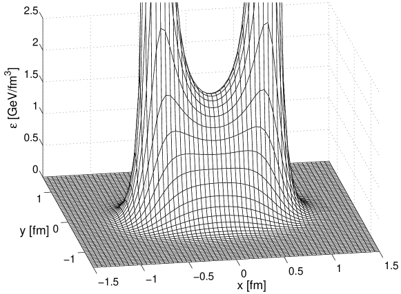
Figure 5: Energy density (integrand of eq. (21)) of the same $q\bar{q}$ string as in fig. 4. A well defined flux tube is stretched between the particles. The scale is chosen to show the flux tube and therefore the strong Coulomb peaks at the quark positions are not seen.

The profiles of the underlying fields $\vec{D}^{3}$, the confinement field $\sigma$ and the dielectric function $\kappa$ at $x=0$ of a 1 fm long $q\bar{q}$ string are shown in fig. 6. On the string axis $\kappa$ and $\sigma$ reach their maximal and minimal value, respectively, and both functions approach to their vacuum values $\kappa_{\text{vac}}$ and $\sigma_{\text{vac}}$, respectively, for $\rho=\sqrt{y^{2}+z^{2}}>0.5\,$fm. The confinement field does not drop down to $\sigma=0$ and therefore the fields are not completely in the perturbative phase. The region where $\kappa$ deviates substantially from its vacuum expectation value ($\rho\leq 0.3\,$fm) defines the bag and consequently the electric flux falls off very fast at the bag boundary.

In the same figure on the right we show the corresponding profile of the energy density. Here we have decomposed the total energy (20) into an electric, a volume and a surface term according to eq. (21).

Figure 6: The profile of the fields (left) and the corresponding energies (right) of a 1 fm string. The electric field $D^{3}$ is scaled to its central value on the axis and the scalar field $\sigma$ to its vacuum value.

The surface energy (dash-dotted line) is maximal on the bag boundary at $\rho\approx 0.3\,$fm, justifying the expression surface energy. The volume energy (dotted line) is distributed more homogeneously within the bag whereas the electric energy (dashed line) falls off quite rapidly.

The energy density in the central plane between the charges at $x=0$ is of special interest as it has been analyzed on the lattice in SU(2) Bali et al. (1995) and also in the framework of the dual color superconductor Maedan et al. (1990); Baker et al. (1991) and in the Gaussian Stochastic Model Kuzmenko and Simonov (2000, 2001); Shoshi et al. (2003). Because of the symmetry all quantities depend only on the distance $\rho$ from the string axis and we may reduce our analysis of the geometry of the flux tube to the shape of this profile function. We follow the reasoning of Bali et al. (1995) and compare the energy profile to both a dipole and Gaussian-like parameterization

$$f_{d}(\rho) = N_{d}(\rho^{2}+\rho_{d}^{2})^{-3}$$ (31a)

$$f_{g}(\rho) = N_{g}\exp[-\ln 2\,(\rho/\rho_{g})^{n}]\quad,$$ (31b)

where $n$ in (31b) is a parameter giving the steepness of the profile. For $n=2$ $f_{g}(\rho)$ is a Gaussian. For small quark separations $R$ perturbative QCD predicts Coulomb-like fields with a characteristic dipole behavior (31a) whereas at large quark separations the field should fall off much faster and the profile should be described better by a generalized Gaussian (31b) with a width at half maximum $\rho_{g}$. We show the profile of the energy density with the parameter set PS-I in fig. 7 together with the best fit of both parameterizations. One can see that the CDM results can be nicely described with a dipole shape for small separations ($R=0.4\,$fm) and with a Gaussian shape ($n=2$) for large separations ($R=1.0\,$fm). It should be noted that the Gaussian shape is only a qualitative guess for the profile. The profile might fall off even faster than described by a Gaussian. To quantify this we will extract below the parameter $n$ from the fit of (31b) to the profile. A value of $n=2$ indicates a pure Gaussian shape and a value $n>2$ is connected to a sharper bounded bag.

Figure 7: The profile of the energy density together with the best fits of the parameterizations (31) fitted over the whole range shown. The profile is better described by a dipole form for small $q\bar{q}$ separations $R$ (left panel) and by a Gaussian form for large $R$ (right panel). In the left fig. we have omitted the dipole peak at the axis to better show the characteristic dipole tail.

In addition to the shape of the flux tube, we will study below the dependence of the total energy (see eq. (21)) as a function of the quark separation $R$, i.e. the $q\bar{q}$ potential $V_{q\bar{q}}(R)$. We compare the calculated CDM $q\bar{q}$ potential to the Cornell potential

$$V_{c}(R)=2C_{F}^{\text{ab}}E_{0}-C_{F}^{\text{ab}}\frac{\alpha}{R}+\tau R.$$ (32)

This potential has been observed on the lattice in SU(2) Bali et al. (1995) and SU(3) Bali and Schilling (1992) and has been used successfully in meson spectroscopy for heavy quarkonia Eichten et al. (1975); Quigg and Rosner (1979); Eichten et al. (1980). It contains the three parameters $E_{0}$, $\alpha$ and $\tau$ which will be determined by a fit to the CDM results. For short distances $R$ one might expect that perturbative one-gluon exchange results of QCD are dominant and thus $V_{c}(R)$ shows the characteristic Coulomb-like $1/R$ potential. To take into account non-perturbative effects $\alpha$ is an effective coupling constant. It has been shown Luscher (1981); Arvis (1983) that there is a $1/R$ correction in the $q\bar{q}$-potential due to quantum-mechanical vibrations of strings around the classical solution. It is beyond the scope of the present paper to predict the corrections to the $R$-dependence within our model. A possible correction of the Coulomb-type is included in the effective coupling constant $\alpha$. For large $R$ the linear term in eq. (32) takes over. It is a consequence of the formation of long linear flux tubes. The string tension $\tau$ expresses the strength of confinement. The constant term is due to the self energy of the quarks. For point-like particles this should diverge but in our numerical realization we have regulated it by the non-zero quark width $r_{0}$. The potential will vanish as $R\rightarrow 0$, because the equal and opposite charge distributions of the quark and the anti-quark start to overlap and to cancel each other. Therefore a Cornell fit is only meaningful for quark separations $R$ substantially larger than $r_{0}$. For convenience we have separated from the Coulomb and the constant term the factor $C_{F}^{\text{ab}}=1/3$. The agreement between our calculations and the Cornell parameterization in eq. (32) will be demonstrated in the next section.

III.2 Variation of the CDM parameters

In the remainder of this section we will discuss the influence of the parameters $B$, $m_{g}$, $\sigma_{\text{vac}}$ and $g_{s}$ on both the energy profile and the total energy. For this purpose we vary all parameters one by one in a certain range while keeping the others at a fixed value given in tab. 2. We calculate the profile for a $R=1.0\,$fm long string as well as the potential $V_{q\bar{q}}(R)$ for varying $R$. From the generalized Gaussian fit to the energy profile we extract the width $\rho_{g}$ and the steepness parameter $n$. From the Cornell fit to the CDM $q\bar{q}$ potential we extract the string tension $\tau$ and the effective coupling constant $\alpha$. The results are collected in tab. 2.

We also study, if the equality between the electric part and the volume part of the string tension is still valid in our model. Note that this equality holds in the simple flux tube model expressed in eq. (29c). For that purpose we also perform a Cornell fit to the different energy fractions $E_{\text{el}}$, $E_{\text{vol}}$ and $E_{\text{sur}}$ separately. From these fits we extract the different parts of the string tension $\tau_{\text{el}}$, $\tau_{\text{vol}}$ and $\tau_{\text{sur}}$. We present the ratios $\beta=\tau_{\text{el}}/\tau_{\text{vol}}$ and $\gamma=\tau_{\text{sur}}/\tau_{\text{tot}}$ also in tab. 2. We find for all parameter combinations a remarkable equality between $\tau_{\text{el}}$ and $\tau_{\text{vol}}$ and the ratio $\beta$ is 1 within a few percent. The surface part of the string tension amounts to roughly $\gamma=0.2$ except in the case when $B\rightarrow 0$ and all other model parameters kept fixed (see first panel in tab. 2). In all simulations shown in this paper we have used $\kappa_{\text{vac}}=10^{-4}$. All string quantities approach its limiting values very rapidly and do not change any more for value $\kappa_{\text{vac}}<10^{-3}$ (see also appendix A.2).

$B^{1/4}\,$[MeV]	$\tau\,\left[\frac{\text{MeV}}{\text{fm}}\right]$	$\beta$	$\gamma$	$\rho_{g}$ [fm]	$n$
0	632	1.07	0.28	0.44	2.8
60	633	1.07	0.28	0.44	2.8
120	642	1.07	0.27	0.43	2.7
180	675	1.06	0.24	0.40	2.5
240	755	1.06	0.19	0.35	2.3
$m_{g}\,$[MeV]	$\tau\,\left[\frac{\text{MeV}}{\text{fm}}\right]$	$\beta$	$\gamma$	$\rho_{g}$ [fm]	$n$
1000	755	1.06	0.19	0.35	2.3
1200	831	1.03	0.19	0.36	2.6
1400	905	1.00	0.20	0.36	3.0
1600	982	1.00	0.21	0.36	3.4
1800	1053	1.00	0.22	0.36	4.0
$\sigma_{\text{vac}}\,$[fm-1]	$\tau\,\left[\frac{\text{MeV}}{\text{fm}}\right]$	$\beta$	$\gamma$	$\rho_{g}$ [fm]	$n$
1.01	755	1.06	0.19	0.35	2.3
1.26	925	1.06	0.21	0.35	2.4
1.51	1110	1.06	0.23	0.34	2.4
1.75	1306	1.06	0.23	0.33	2.3
2.00	1511	1.06	0.24	0.32	2.3
$g_{s}$	$\tau\,\left[\frac{\text{MeV}}{\text{fm}}\right]$	$\beta$	$\gamma$	$\rho_{g}$ [fm]	$n$
0.2	100	0.94	0.20	0.21	1.9
0.5	223	0.97	0.20	0.24	2.0
1.0	418	1.06	0.19	0.29	2.2
1.5	591	1.06	0.19	0.32	2.3
2.0	755	1.06	0.19	0.35	2.3
2.5	911	1.05	0.18	0.37	2.4
3.0	1062	1.05	0.18	0.39	2.4
3.5	1212	1.04	0.18	0.41	2.3
4.0	1356	1.04	0.18	0.42	2.3
5.0	1637	1.04	0.17	0.43	2.2

Table 2: The string tension $\tau$, the string width $\rho_{g}$ and the steepness parameter $n$ for varying model parameters. The ratios $\beta$ and $\gamma$ are defined in the text. We vary the parameters one by one and keep the other fixed at $B^{1/4}=240\,$MeV, $m_{g}=1000\,$MeV, $\sigma_{\text{vac}}=1.01\,\text{fm}^{-1}$ and $g_{s}=2$, respectively. Throughout this work we use $\kappa_{\text{vac}}=10^{-4}$.

Bag constant $B$:

We start with a variation of the scalar potential $U$ (see eq. (7)). We vary $B$ from $B=0$ to the maximal value allowed by eq. (9) $B^{1/4}=240\,$MeV (first panel in tab  2). At the lower value $U(\sigma)$ has two degenerate vacua and at the higher value it has only an inflection point at $\sigma=0$ (see dashed lines in fig. 2). From the simple bag model, eq. (29), we would expect the string tension to increase quadratically with $B^{1/4}$ and the string width to decrease with $B^{-1/4}$ for increasing values $B$. Instead the string constant $\tau$ grows only weakly over the whole range and is non-zero at $B=0$. Note that for $B=0$ the profile of the volume energy $U(\rho)$ is non-zero everywhere and a string of finite width is formed. The string radius shows the expected tendency though the decrease starts only for $B^{1/4}\geq 120\,$MeV. The profile is steeper than a Gaussian for small $B$ ($n=2.8$) and approaches a Gaussian for larger values.

Glueball mass $m_{g}$:

When we fix the bag constant and vary only the glueball mass $m_{g}$ (second panel in tab. 2) the string tension increases roughly linearly with $m_{g}$. The string width stays constant over the whole tested range $m_{g}=(1000\ldots 1800)\,$MeV in tab. 2. Simultanously the steepness $n$ of the profile increases strongly up to $n=4$. In the limit $m_{g}\rightarrow\infty$ the local maximum $U(\sigma)$ rizes infinetely and the confinement field $\sigma$ is restricted to be either $\sigma=0$ or $\sigma=\sigma_{\text{vac}}$. In this case we expect to reproduce the bag with sharp boundaries discussed in eq. (29). Of course this is not reached in the CDM but we observe the tendency in the rise of $n$. We see that the string tension is more affected by the mass $m_{g}$ than by the bag constant $B$ and that vice versa the string radius is nearly independent on $m_{g}$ but decreases with $B$. Note that the glueball mass has no analog in the bag model, where the shape of the flux tube is assumed to be rectangular.

Vacuum value $\sigma_{\text{vac}}$:

Qualitatively the string quantities should depend in the same way on the vacuum value $\sigma_{\text{vac}}$ as on $m_{g}$. If we increase $\sigma_{\text{vac}}$ from its minimal allowed value given by eq. (9) to higher values a local maximum in the scalar potential $U(\sigma)$ develops (see dash-dotted curves in fig. 2). In this case the stiffness $m_{g}$, i.e. the curvature of the potential at $\sigma_{\text{vac}}$ is unchanged. The increasing surface energy related to the larger gradient in the confinement field $\sigma$ reduces the string radius $\rho_{g}$. In the tested range the radius decreases from $\rho_{g}=0.35\,$fm to $\rho_{g}=0.32\,$fm (see third panel in tab. 2). Though the decrease in the string radius is not very large, the string tension doubles its value from 755 MeV/fm to 1511 MeV/fm. The steepness of the energy profile is rather independent from $\sigma_{\text{vac}}$.

Coupling constant $g_{s}$:

The couping $g_{s}$ determines directly the strength of the electric flux in the string. From eq. (29) we expect the string tension to rize linearly with $g_{s}$ and the string radius to increase proportional to $\sqrt{g_{s}}$. Indeed we find a nearly perfect linear behavior of $\tau$ (4th panel in tab. 2) and also the string width has the expected qualitative behavior. The linear dependence between the string tension and the coupling $g_{s}\sqrt{C_{F}}$ is valid in general for all bag-like models Lucini and Teper (2001); Hansson (1986). For the coupling $g_{s}$ we also look at the $q\bar{q}$ potential at small quark separations $R$, i.e. we extract the parameter $\alpha$ in the Coulomb term of the Cornell potential which is dominant for $R<0.2\,$fm. For small $R$ the bag has almost spherical shape and the $q\bar{q}$ interaction can be treated perturbatively. In fig. 8 we show the Coulomb parameter for varying $g_{s}$. The electric part $\alpha_{\text{el}}$ (circles) is perfectly described by the perturbative result $\alpha_{\text{el}}=\frac{g_{s}^{2}}{4\pi}$ (dashed line). The surface contribution $\alpha_{\text{sur}}$ (triangles) does not follow the quadratic behavior and seems to grow more linearly and rather slowly. It thus acts as a non-perturbative correction to the perturbatively expected Coulomb interaction $\alpha=\frac{g_{s}^{2}}{4\pi}+\alpha_{\text{sur}}$. The volume energy increases linearly with $R$ and thus the corresponding Coulomb parameter is compatible with zero and not included in the figure.

Figure 8: The Coulomb coupling parameter $\alpha$ extracted from the Cornell fit for different $g_{s}$. The electric part (dots) is in perfect agreement with the one-gluon exchange result (line). The surface part (triangles) contributes only a small amount to the Coulomb potential and therefore the effective $\alpha$ (squares) rises quadratically with $g_{s}$.

	$B$	$m_{g}$	$\sigma_{\text{vac}}$	$g_{s}$
$\tau$	$\nearrow$	$\uparrow$	$\uparrow$	$\uparrow$
$\rho_{g}$	$\downarrow$	—	$\searrow$	$\uparrow$
$n$	$\downarrow$	$\uparrow$	—	—

Table 3: The reaction of string tension $\tau$, the string width $\rho_{g}$ and the steepness $n$ on increasing model parameters.

We end this section in summarizing the reaction of the string tension $\tau$, the string width $\rho_{g}$ and the steepness of the profile on the parameter variation in tab. 3.

IV $q\bar{q}$ strings

IV.1 CDM and lattice results

After having analyzed the influence of the model parameters on the shape and the energy of $q\bar{q}$ strings, we compare the CDM results to lattice calculations. We first describe $q\bar{q}$ strings to fix the parameters and later on turn to $qqq$ systems in section V.

In Bali et al. (1995) detailed studies of long flux tubes were made in SU(2) lattice gauge theory. The authors compared the profile of the action and the energy density of strings of varying length. We will tune the parameters of our model to reproduce the phenomenological value of the string tension $\tau$ and to desribe the energy profile of a 1 fm long $q\bar{q}$ string as good as possible within our model. For the profile a measure for the agreement of our calculations and lattice results is the quantity $(\Delta\varepsilon)^{2}=\sum_{i}[\varepsilon(\rho_{i})-\varepsilon_{\text{lat}}(\rho_{i})]^{2}$, where $\varepsilon_{\text{lat}}(\rho_{i})$ is the energy density given at discrete radial distances $\rho_{i}$ (see fig.24 in Bali et al. (1995)). To find the optimal set of parameters we scan a wide range of our parameter space and minimize $\Delta\varepsilon$ with the constraint to reproduce the string tension $\tau=980\,$MeV/fm.

Doing this we follow three different strategies. In the first we treat all model parameters from tab. 3 as free parameters, determined from the minimization of $\Delta\varepsilon$ only. In this case we do not lean on the heuristic interpretation of $B$ as the bag constant and $m_{g}$ as the glueball mass. This results in parameter set PS-I in tab. 4. In the second we take $B$ and $m_{g}$ as the bag constant and the glueball mass, respectively. The former is chosen to be $B^{1/4}=240\,$MeV as found in QCD sum rules Shifman et al. (1979a, b) and also in another bag-like analysis Hasenfratz et al. (1980a, b). The latter is restricted to be at $m_{g}=(1500-1700)\,$MeV as given by SU(3)-lattice results for the scalar glueball mass Morningstar and Peardon (1997); Michael (1999). This leaves only $g_{s}$ and $\sigma_{\text{vac}}$ as free parameters and $m_{g}$ in the small range mentioned to find the minimum of $\Delta\varepsilon$ and we get parameter set PS-II in tab. 4. In the last variation we restrict additionally the coupling constant to $g_{s}=3.3$ in order to reproduce not only the string tension but also the Coulomb parameter $\alpha=0.29$ of the Cornell potential as calculated on the lattice Bali (2001). The last free parameter $\sigma_{\text{vac}}$ is varied in this case to get the right string tension and we obtain parameter set PS-III. Of course the deviation of the CDM energy profile to the lattice result increases from parameter set PS-I to PS-III. The three different parameter sets therefore express a quantitative variation of the model predictions. With the given parameters the scalar potential $U(\sigma)$ changes as shown in fig. 9. Within PS-I (solid curve) there is only a negligible relative maximum in the potential, and it vanishes exactly for PS-III (dash-dotted line). In the second parameter set a pronounced relative maximum develops (dashed line). We note that the values of the bag constant $B$ are much larger than the value $B^{1/4}=145\,$MeV chosen in the original MIT bag model Chodos et al. (1974a) and also in a previous CDM analysis Traxler et al. (1999). Recall that in Traxler et al. (1999) the string profile is much broader and inconsistent with lattice results. The vacuum value for the dielectric constant is $\kappa_{\text{vac}}=10^{-4}$ for all parameter sets. We show in appendix A.2, that the physical quantities of the string do not change anymore for smaller values of $\kappa_{\text{vac}}$.

Figure 9: The scalar potential $U(\sigma)$ for the three parameter sets given in tab. 4.

No.	$B$	$m_{g}$	$\sigma_{\text{vac}}$	$g_{s}$	$\kappa_{\text{vac}}$
I	(260 MeV)4	1000 MeV	1.29 fm-1	2.0	$10^{-4}$
II	(240 MeV)4	1500 MeV	1.13 fm-1	1.8	$10^{-4}$
III	(240 MeV)4	1700 MeV	0.59 fm-1	3.3	$10^{-4}$

Table 4: CDM parameter sets used in the description of $q\bar{q}$ strings and $qqq$ baryons.

In fig. 10 we show the result of the three different fitting procedures for the 1 fm long $q\bar{q}$ string. The profile for PS-I runs smoothly through the lattice points showing the high quality of the fit. The profile of PS-II has roughly the same half maximum width $\rho_{1/2}=0.32\,$fm but a steeper profile due to the higher glueball mass. In the last case for PS-III the flux tube is much broader with a half maximum width $\rho_{1/2}=0.45\,$fm. Due to the large coupling $g_{s}$ for PS-III we cannot push the string radius to smaller sizes while keeping the string tension at the prescribed value.

Figure 10: The energy density profile of a 1 fm string. The profiles for PS-I and PS-II have a half maximum width of $\rho\approx 0.35\,$fm although the slope is steeper for PS-II. PS-III results in a broader string. Lattice results taken from Bali et al. (1995).

To analyze further the different parameter sets, we decompose the total energy according to eq. (21) into the different energy parts. The result is shown in the profiles in fig. 11. In all cases the electric energy builds up most part of the total energy. Note that this is not in contradiction to the previous result that the electric and the volume part of the string tension are of the same magnitude. The string tension is by definition $\tau=\frac{dE_{\text{tot}}}{dR}$ and not the energy of the central slice of the string. This would be the same only for strings with constant width, which is not the case for finite quark separations.

For PS-I (left panel) the volume energy (dash-dotted lines) never exceeds the bag constant, whereas for PS-III (right panel) it has a wide range inside the bag, where it is constant and equal to $B$. For PS-II (central panel) we see that on the string axis, the volume energy comes close to the local minimum at $\sigma=0$, which is seen in the central dip. The surface energy is strongly pronounced for PS-II and the two peaks are clearly separated for PS-III. In the last case the interior of the bag is therefore much more pronounced than in the other two parameter sets.

Figure 11: The decomposition of the energy profile into the different energy components for $R=1\,$fm.

The underlying fields $D^{a}(\rho)$, $\sigma(\rho)$ and the dielectric constant $\kappa(\rho)$ for this 1 fm string are shown in fig. 12. For all parameter sets the scalar field never reaches the perturbative situation $\sigma=0$ within the string. According to that $\kappa$ is never exactly equal to 1. For PS-I and PS-II it has only a value of $\kappa=0.75$ and $\kappa=0.85$ respectively. Only for PS-III the perturbative value $\kappa\apprle 1$ is reached. Of course also the fields are broader as compared to the other two parameter sets.

The dielectric constant $\kappa(\rho)$ has roughly the same shape as the electric field $D^{a}(\rho)$. This indicates already that according to eq. (30) the string picture should be valid for $R=1\,$fm.

Figure 12: The scaled profiles of $\vec{D}^{a}$, $\sigma$ and $\kappa(\sigma)$ of a 1 fm string. The profiles of $\kappa$ and $\vec{D}^{a}$ have roughly the same shape as expected from eq. (30) for long flux tubes. $\kappa$ reaches 1 only for PS-III and is smaller than 1 for PS-I and PS-II.

One can expect that for increasing $q\bar{q}$ distances $R$ the profiles evolve to some stable shape and that the asymptotic relation eq. (30) between electric field and dielectric constant should become increasingly accurate. To study this issue we show the profile of the total energy density for different quark separations $R$ in fig. 13. For small $R$ we see the strong Coulomb peak. But for separations $R>1.2\,$fm the string profile does not change strongly anymore and the asymptotic profile is nearly reached.

Figure 13: The profile of the energy density for different $q\bar{q}$ separations $R$ given in the figure. The asymptotic shape is nearly reached for $R\geq 1.2\,$fm. For small $R$ the Coulomb peak is seen.

This can be seen as well in fig. 14, where we have plotted the ratio of the normalized profiles of $D^{3}$ and $\kappa$ in the range $|y|\leq 0.7\,$fm, where the string is located. According to eq. (30) this should be constant equal to unity for large $R$. Indeed this ratio becomes increasingly flat and equal to one for increasing $R$.

Figure 14: The ratio of the electric field $D^{3}$ to the dielectric constant $\kappa$, each normalized to its central value. The asymptotic relation in eq. (30) is nearly reached for $q\bar{q}$ separations $R\geq 1.2\,$fm.

To complete the discussion of the energy density profile we compare the full half maximum width $\Delta=2\rho_{g}$ extracted from the Gaussian fit to the results obtained in lattice SU(2) calculations Bali et al. (1995) for various string lengths $R$. Here we have fixed the steepness parameter to $n=2$ to be consistent with the analysis in Bali et al. (1995). In fig. 15 one sees that the calculated string widths are compatible with the lattice data for parameter sets PS-I and PS-II. Again the string width is overestimated for PS-III due to the large coupling $g_{s}$. First the width increases rapidly for small separations $R\leq 0.8\,$fm. For the largest quark separation $R=2\,$fm the width has a value $\Delta=0.78\,$fm and $\Delta=0.68\,$fm for parameter sets PS-I and PS-II, respectively, and the width seems to saturate. The width for PS-III is $\Delta=0.97\,$fm and still increases slightly. We note that qualitatively this behavior is consistent with the lattice string picture Kogut and Susskind (1975); Kogut et al. (1981), where a logarithmic increase of the string width with the quark separation $R$ is predicted.

Figure 15: The Gaussian width of the flux tube as a function of quark separation. For parameter sets PS-II the width saturates at $\Delta\approx 0.7\,$fm. For PS-I and PS-III the width of the profile still increases slightly for separations up to $R=2\,$fm. Lattice data are taken from Bali et al. (1995).

IV.2 CDM and the Dual Color Superconductor

In this part of the discussion of $q\bar{q}$ strings we make a connection to the Dual Color Superconductor model (DCS) known also as the dual Ginzburg-Landau model. In this model color flux tubes between a quark and an anti-quark are formed by the interaction to a scalar field carrying a magnetic charge. Those Abrikosov-Nielsen-Olesen vortices Abrikosov (1957); Nielsen and Olesen (1973); Ripka (2004) are stabilized by a circular magnetic current

$$\vec{\jmath}_{\text{mag}}=\vec{\nabla}\times\vec{E}_{\text{DCS}}$$ (33)

flowing around the string axis. It is speculated that such a magnetic current is produced by the condensation of magnetic monopoles which can be constructed in non-Abelian gauge theories ’t Hooft (1974); Polyakov (1974). The DCS flux tube has a characteristic profile of the electric field $\vec{E}_{\text{DCS}}=E_{\text{DCS}}(\rho)\vec{e}_{x}$. To compare our results with the DCS model we first note that by construction of the electromagnetic field tensor $F^{\mu\nu,a}$ in eq. (1d) the curl of the electric field $\vec{E}$ vanishes identically for static configurations. However, by a simple redefinition of the field tensor $F^{\mu\nu,a}\rightarrow G^{\mu\nu,a}=\kappa(\sigma)F^{\mu\nu,a}$ one may define a quantity

$$j_{\text{mag}}^{\mu,a}:=\partial_{\nu}{\cal G}^{\mu\nu,a}\neq 0\quad,$$ (34)

where ${\cal G}^{\mu\nu,a}={\textstyle\frac{1}{2}}\epsilon^{\alpha\beta\mu\nu}G^{\mu\nu,a}$ is the dual field tensor to $G^{\mu\nu,a}$. This quantity exactly behaves as a magnetic current and the spatial part is in our standard notation $\vec{\jmath}^{\;a}_{\text{mag}}=\vec{\nabla}\times\vec{D}^{a}$. In the absence of magnetic fields there is no magnetic charge density, i.e. $\rho^{a}_{\text{mag}}=\vec{\nabla}\cdot\vec{H}^{a}=0$. In our model the magnetic current is connected to the electric displacement $\vec{D}^{a}$ whereas it is connected to the electric field $\vec{E}_{\text{DCS}}$. Thus $\vec{D}^{a}$ and $\vec{E}_{\text{DSC}}$ are confined in the two models and we compare $\vec{D}^{a}$ with $\vec{E}_{\text{DCS}}^{a}$. In Bali et al. (1998); Gubarev et al. (1999); Koma et al. (2003a) a detailed study of the electric profile of a $q\bar{q}$ configuration was made within lattice gauge theory and it was found that the profile can be described very well by the DCS model. In addition the authors found a magnetic current $\vec{\jmath}_{\text{mag}}$ fulfilling eq. (33). In fig. 16 we show the lattice results of the electric profile (triangles) compared to those obtained within our calculations. We find only a qualitative agreement, where again PS-I and PS-II reproduces the electric profile better than PS-III.

Figure 16: Comparison of the profile of the electric displacement $\vec{D}$ within CDM and the profile of the electric field $\vec{E}$ found on the lattice.

The spatial part of the magnetic current constructed in eq. (34) in the central plane between the two particles at $x=0$ is displayed in fig. 17 (left). In a cylindrical basis it has only an azimuthal component. One sees the circulating structure of the current which gives this flux tube the name vortex in the DCS model. We show our results for the profile of the magnetic current with the different parameter sets and compare it to lattice data Bali et al. (1998) in the right panel of figure 17. The maximal values are shifted to larger values of $\rho$ compared to lattice data. Parameter set PS-III develops a pronounced current only on the surface of the string. In identifying the magnetic current in our model we can make a link between our model and the model of the dual color superconductor. It should be noticed that the CDM model is formulated on the basis of the gauge potentials $A_{\mu}^{a}$ which can be directly related to the gluon fields of QCD, whereas the DCS model is formulated in the dual gauge potentials. In this sense the model gauge fields in the CDM can be more easily interpreted as the QCD gluon fields than in the dual superconductor model.

Figure 17: The circular magnetic current $\vec{\jmath}_{\text{mag}}=\nabla\times\vec{D}^{a}$ (left) and the scaled profile of it (right). For PS-III the current is locate at the surface of the bag. Lattice results taken from Bali et al. (1998).

IV.3 The $q\bar{q}$ potential

We can quantify the analysis of a string further by showing the total energy $E_{\text{tot}}$ of the string as a function of the $q\bar{q}$ distance $R$ in fig. 18 together with the electric, the volume, and the surface part of the energy. All parts of the energy show a linear rise with the $q\bar{q}$ separation for $R\gtrsim 0.2\,$fm. Due to the self energy of the nearly point-like particles the electric energy is larger than the other two energy contributions. This is most obvious for PS-III where the coupling constant $g_{s}$ is largest. We have performed a Cornell fit according to eq. (32) to the total energy $E_{\text{tot}}$ and to the single energy parts separately. The extracted parameters $E_{0},\alpha$ and $\tau$ and the corresponding values for the electric, volume and surface energy contributions are listed in the first three columns in tab. 5. It should be noted, that the self energy $E_{0}$ depends on the width of the particles. The given values correspond to a Gaussian width of $r_{0}=0.02\,$fm which can still be resolved on the used computational grid.

The string tension is $\tau\approx 980\,$MeV/fm as the model parameters were fitted to this value. The effective strong coupling $a_{F}=C_{F}^{\text{ab}}\alpha$ isolated from the Cornell fit to the $q\bar{q}$ potential ranges from 0.12 with PS-II to 0.30 with PS-III. A Cornell fit obtained from meson spectroscopy gives an effective Coulomb coupling ranging from $a_{F}=0.25$ Eichten and Gottfried (1977) to $a_{F}=0.5$ Quigg and Rosner (1979). The latter estimate included both the charm and the bottom quark mesons. In the MIT bag model DeGrand et al. (1975) and in the CDM hadronization study Traxler et al. (1999) an effective coupling $a_{F}=3.0$, and $a_{F}=2.6$ were used, respectively. Together with the small value of the bag constant used in these works the string width amounts to $\rho=1.9\,$fm and $\rho=1.5\,$fm, respectively, which is large as compared to the value of $\rho=0.35\,$fm obtained on the lattice Bali et al. (1995). In a further bag model analysis Hasenfratz et al. (1980a) the authors extracted a value $a_{F}=0.38$ for the coupling constant. The coupling isolated from a Cornell fit to lattice data prefers a value of $a_{F}=0.3$ Morningstar and Peardon (1997); Bali (2001). The CDM values for the coupling in tab. 5 underestimates this value for $a_{F}$ for PS-I and PS-II. Parameter set PS-III was designed in order to reproduce the Cornell potential, so the agreement is optimal here.

Figure 18: The $q\bar{q}$ potential $E(R)$ for the different parameter sets together with the different fractions of the energy and the Cornell fit to the total energy.

	fundamental			adjoint			ad/fund
	PS-I	PS-II	PS-III	PS-I	PS-II	PS-III	PS-I	PS-II	PS-III
$e_{D}$ [MeV]	388	294	757	961	763	2202	2.5	2.6	2.9
$a_{D}$	0.18	0.12	0.30	0.41	0.31	0.87	2.3	2.7	2.9
$\tau$ [MeV/fm]	979	982	980	1548	1502	1586	1.6	1.5	1.6
$e_{D}^{\text{el}}$ [MeV]	297	235	726	833	679	2163	2.8	2.9	3.0
$a_{D}^{\text{el}}$	0.12	0.09	0.29	0.34	0.28	0.86	2.7	3.1	3.0
$\tau_{\text{el}}$ [MeV/fm]	404	390	424	640	585	695	1.6	1.5	1.6
$\tau_{\text{vol}}$ [MeV/fm]	381	380	435	610	588	717	1.6	1.5	1.7
$e_{D}^{\text{sur}}$ [MeV]	108	78	47	151	108	63	1.4	1.4	1.4
$a_{D}^{\text{sur}}$	0.07	0.05	0.03	0.10	0.07	0.04	1.4	1.4	1.4
$\tau_{\text{sur}}$ [MeV/fm]	195	212	122	299	328	174	1.5	1.5	1.4

Table 5: The parameters $e_{D}=C_{D}E_{0}$, $a_{D}=C_{D}\alpha$ and $\tau$ extracted from the Cornell fit to the total energy as well as to the different energy contributions separately. The first block of three columns belongs to quarks in the fundamental representation ($D=F$), the second to quarks in the adjoint representation ($D=A$) and the last shows the ratio of both.

After having shown the CDM results for the $q\bar{q}$ potential, we would like to comment on the so called Casimir scaling hypothesis Ambjørn et al. (1984b, a); Bali (2000); Deldar (2000); Lucini and Teper (2001); Koma et al. (2003b). According to this hypothesis the $q\bar{q}$ potential should scale with the quadratic Casimir operator $C_{D}$ of the static sources $q$ and $\bar{q}$ in the representation $D$ . For small quark separations $R$ the potential is dominated by the perturbative Coulomb term which already scales with $C_{D}$. For larger distances this cannot be deduced from perturbation theory and must be shown numerically on the lattice. This has been done for various representations $D$ in Michael (1998); Kratochvila and de Forcrand (2003); Bali (2000); Deldar (2000). For the adjoint representation for example one should expect the string tension to scale with $(C_{A}/C_{F})\,\tau_{F}=2.25\tau_{F}$. This can hold if at all only for intermediate quark distances, as the adjoint potential should saturate for separations larger than some critical distance $R_{c}$ Michael (1998); Kratochvila and de Forcrand (2003). Numerical values for the string tension $\tau_{D}$ have been given in Bali (2000) and in Deldar (2000). An unambiguous confirmation for the scaling hypothesis has not been seen. The deviations from scaling where found to be (2-5)% Bali (2000) and (10-15)% Deldar (2000) for various representations. Interestingly, all results lie consistently under the value predicted by Casimir scaling. For the ratio of the adjoint string tension to the fundamental one a value $\tau_{A}/\tau_{F}=1.97\pm 0.01\pm 0.12$ was calculated in Deldar (2000), with the respective statistical and systematic errors. This corresponds to a deviation from Casimir scaling by $(12\pm 6)\%$.

In the CDM we can simulate adjoint quarks. We simply assign the adjoint charge to the three quarks, i.e. the sum of the charges of a quark and an anti-quark. The numerical values are given in tab. 6. Note that one can construct only 6 charged adjoint quarks. The other two members of the octet are uncharged. We have already seen that the Coulomb term in our potential scales with the square of the coupling constant $g_{s}$ or, rephrased in terms of the Casimir operator, scales with the Casimir Operator. The string tension, however, was found to scale with $g_{s}$ and $\sqrt{C_{D}^{\text{ab}}}$, respectively. Therefore the adjoint string tension should be $\tau_{A}=\sqrt{C_{A}^{\text{ab}}/C_{F}^{\text{ab}}}\,\tau_{F}\approx 1.7\tau_{F}$, where we have used the Abelian Casimir values $C_{F}^{\text{ab}}=1/3$ and $C_{A}^{\text{ab}}=1$.

We have performed the simulation for the adjoint string and isolated the Cornell parameters $e_{A}=C_{A}E_{0}$ and $a_{A}=C_{A}\alpha$ and $\tau_{A}$. The results of these values for the different parameter sets are given in tab. 5 (2nd block of three columns) together with the corresponding ratios (3rd block). The short range Cornell parameters of the electric energy have approximately the expected ratio of 3. Also the adjoint string tension as well as the different parts of the energy scale with the expected value of $\sqrt{C_{A}^{\text{ab}}/C_{F}^{\text{ab}}}=1.7$ which has to be compared to the SU(3) scaling value $C_{A}/C_{F}=2.25$ and the empirical value $\tau_{A}/\tau_{F}=1.97$ Deldar (2000). In SU(2) lattice calculations Kratochvila and de Forcrand (2003) a clear deviation from Casimir scaling was detected. We conclude that Casimir scaling is not seen in our model which is in accordance with all bag models Hansson (1986); Johnson and Thorn (1976); Lucini and Teper (2001). Casimir scaling is also not seen within the Dual Color Superconductor model, when the superconductor is on the border between first and second type Ball and Caticha (1988); Koma et al. (2003b), i.e. where lattice results agree with this model the best. We note that it is also qualitatively in line with the tendency of lattice calculations to underestimate the adjoint string tension systematically.

We note in this context that the deviation is an intrinsic feature of the CDM, which is due to the larger fluxtube cross section in the present of charges in higher representation. If in the future lattice data will show that Casimir scaling would hold for the $q\bar{q}$-potential, this would be a strong argument against all bag-like models in favor of models with explicit scaling Shoshi et al. (2003). In the meantime we regard those type of models as competitive.

color	$q^{3}$	$q^{8}$
$r\bar{g}$	$1$	$0$
$r\bar{b}$	$1/2$	$\sqrt{3}/2$
$g\bar{b}$	$-1/2$	$\sqrt{3}/2$
$g\bar{r}$	$-1$	$0$
$b\bar{r}$	$-1/2$	$-\sqrt{3}/2$
$b\bar{g}$	$1/2$	$-\sqrt{3}/2$

Table 6: Color charge of color sources in the adjoint reprentation.

V $qqq$ baryons

Now that we have fixed the model parameter to reproduce lattice results for $q\bar{q}$ strings, we go on to describe baryon-like $qqq$ configurations. It has been discussed for a long time Cornwall (1977); Sommer and Wosiek (1984); Cornwall (1996); Kuzmenko and Simonov (2001); Alexandrou et al. (2002a); Takahashi et al. (2002), whether the flux tubes stretching between the quarks will connect the particles pairwise with a $qq$ string, indicating 2-particle interactions, or whether they are connected via a central point giving rise to a real 3-particle force. In the former case the geometry of the system will show a triangular or $\mathsf{\Delta}$-like shape, whereas in the latter it will have a Y-like shape. The situation is depicted in figure 19. Although our model is formulated in the Abelian approximation we must not naively assume that the flux tubes are a simple superposition of three $qq$ flux tubes. The non-linear interactions with the dielectric medium might deform the flux tube to show a Y-like geometry.

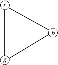
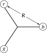
Figure 19: $\mathsf{\Delta}$-shape (left) and Y-shape (right) of the $qqq$ configuration. In the Y-geometry each of the three quarks is connected to the central point with the same string as in the $q\bar{q}$ case. In the $\mathsf{\Delta}$-geometry the quarks are connected pairwise by a modified flux tube.

This question has been studied on the level of the potential within lattice SU(3) Bali (2001); Takahashi et al. (2002); Alexandrou et al. (2002b) and on the level of the fields Ichie et al. (2003a, b); Bornyakov et al. (2003). Depending on the shape the potential will scale characteristically with the 2-particle distance $R$. To parameterize it in the spirit of the Cornell potential eq. (32) we decompose the potential into a constant term due to the quark self energy, a Coulomb-like short distance term and a confining linear term. The constant term scales with the number of particles in the system and the short range term scales with the sum over the two particle Coulomb interactions. The Coulomb interaction is accompanied by the same color factor $\frac{1}{3!}\epsilon_{\alpha\beta\gamma}\epsilon_{\sigma\tau\gamma}t^{a}_{\alpha\sigma}t^{a}_{\beta\tau}=-C_{F}^{\text{ab}}/2$ as in eq. (26b).

The confining term scales with the total length of the flux tubes spanned between the quarks, which is different in the two geometries (see fig. 19). In the case of the Y-geometry a $q\bar{q}$-like string is connected to each of the three quarks, meeting at a central point. In the case of three quarks sitting on the corners of an equilateral triangle with length $R$, the length of each of the flux tubes is equal to $R/\sqrt{3}$. This yields eq. (35a) below.

In the $\mathsf{\Delta}$-geometry two flux tubes are connected to each quark, so there is a reduced electric flux in each $qq$ string compared to that of the $q\bar{q}$ string. Due to the symmetry of color exchange the total energy per unit length stored in the two strings must be of equal size. To deduce this relative strength of the modified flux tube we apply a limiting procedure. Think of two of the quarks approaching each other, e.g. the $r$-quark and the $g$-quark. As they come together we end up with a quark–diquark system but with two $qq$ strings lying on top of each other. As the diquark behaves exactly like an anti-quark the linear part scales with the known string tension $\tau$ and we conclude that the $qq$ flux tube has a string tension reduced by a factor of two. This factor is also obtained in Cornwall (1996). Note that we have assumed here, that the flux in each $qq$ string is independent of the third quark position. The $qqq$ potential may now be parameterized as:

$$V_{\mathsf{Y}} =3C_{F}^{\text{ab}}E_{0}-\frac{C_{F}^{\text{ab}}}{2}\sum_{i<j}\frac{\alpha}{|\vec{r_{i}}-\vec{r}_{j}|}+\tau\sum_{i}|\vec{r_{i}}-\vec{r}_{c}|$$ (35a)

$$=3C_{F}^{\text{ab}}E_{0}-3\frac{C_{F}^{\text{ab}}}{2}\frac{\alpha}{R}+\sqrt{3}\tau R$$

$$V_{\mathsf{\Delta}} =3C_{F}^{\text{ab}}E_{0}-\frac{C_{F}^{\text{ab}}}{2}\sum_{i<j}\frac{\alpha}{|\vec{r_{i}}-\vec{r}_{j}|}+\frac{1}{2}\tau\sum_{i<j}|\vec{r_{i}}-\vec{r}_{j}|$$ (35b)

$$=3C_{F}^{\text{ab}}E_{0}-3\frac{C_{F}^{\text{ab}}}{2}\frac{\alpha}{R}+\frac{3}{2}\tau R$$

Here $\vec{r}_{i}$ are the positions of the particles and $\vec{r}_{c}$ is the position of the flux tube junction in the Y-case. The parameters $E_{0}$, $\alpha$ and $\tau$ are the ones extracted from the fit to the $q\bar{q}$ string in the previous section and listed in tab. 5. The respective last equality in eq. (35) holds for the quarks sitting on the corners of an equilateral triangle. The effective string tension $\tau_{\mathsf{\Delta}}=(3/2)\,\tau$ is smaller than $\tau_{\mathsf{Y}}=\sqrt{3}\tau$ making it the preferable configuration although it is only an effect of 14%.

This picture is surely oversimplified, since the flux tubes are not strings with zero transverse extent. The single flux tubes will overlap due to their finite width $\rho$ and the true fields will lead to a smearing of the two extreme configurations at least for quark distances only slightly greater than the flux tube width. Both the finite size of the flux tubes and the tininess of the overall effect makes it hard to decide on the lattice, which might be the more appropriate description. In references Bali (2001); Alexandrou et al. (2002a) a $\mathsf{\Delta}$-like scaling of the potential was found suggesting an effective 2-particle interaction, whereas in Takahashi et al. (2002); Bornyakov et al. (2004) the baryonic string tension was better described by Y. In another calculation Alexandrou et al. (2003) neither ansatz give a proper description of the potential for all quark separation. Instead the authors stated that the potential is of the $\mathsf{\Delta}$-type for small separations $R$ and of $Y$-type for large $R$.

In the following we first show the fields for the three-quark system with the symmetry shown in figure 19 as calculated in CDM. Then we will compare the $qqq$ potential obtained within CDM to those constructed in eq. (35) using the Cornell parameters $E_{0},\alpha$ and $\tau$ obtained in section IV. Finally we will perform a new fit of our Cornell parameters to the $qqq$ potential. We would like to stress here, that in a renormalization group derivation of the dielectric model Mack (1984); Chanfray et al. (1989); Mathiot et al. (1989) an additional colorless vector field appears. This vector field is relevant in the calculations of systems with non-vanishing baryon-density. However in the spirit of the present work, we are interested in the pure glue $qqq$-type flux tubes with fixed external charges, where the neglect of this additional term is justified.

In figure 20 we show the color electric field of a configuration, where the rightmost, uppermost and lowermost quarks have color blue ($b$), red ($r$) and green ($g$), respectively. The pairwise quark distance is equal to $R=1.7\,$fm. In the left (right) part of the figure the electric 3-field (8-field) $\vec{D}^{3/8}$ is shown. As the $b$ quark has no 3-charge component the 3-field connects only the $r$ and the $g$ quark. But as can be seen clearly, due to the existence of the $b$ quark, the confinement field $\sigma$ is reduced in the whole region between the three quarks and the electric 3-flux is bent towards the $b$ quark. The electric flux of the 8-field connects all three quarks. The $r$ and the $g$ quark are equal sources of this field and the flux ends on the $b$ quark. Again the flux is deformed compared to the $q\bar{q}$ flux tube and is pushed towards the center of the $qqq$ configuration. We have included in the same picture the contour lines for the dielectric function $\kappa(\sigma)$. One can see that the maximal value of $\kappa$ (neglecting the peak positions at the quarks) shows a Y-type shape, and falls off to zero towards the sides of the triangle within a range of 0.5 fm.

Figure 20: The color fields of a $qqq$ baryon. The red/green/blue quark is the upper/lower/rightmost one. The $\vec{D}^{3}$ flux (left) connects only the red and the green quark, whereas the $\vec{D}^{8}$ flux (right) connects all three quarks. The flux is bent into the center of the configuration. Solid lines are the equipotential values of $\kappa$.

As we have argued in section II the electric field shown in figure 20 is not an invariant quantity under the global color symmetry. The strength and the direction of the fields depend on the specific arrangement of the colors in the $qqq$ state. We have included the picture of the electric field only to give an insight to the underlying mechanism of flux tube formation. The relevant quantity again is the energy density of the system. As in the $q\bar{q}$ case we split the total energy into electric, volume and surface terms (21).

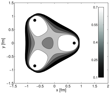
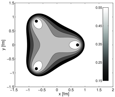
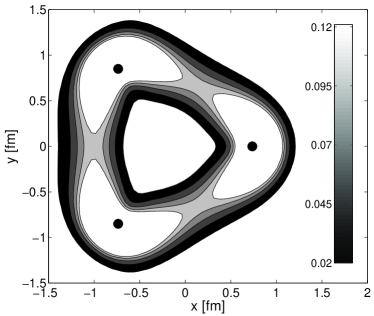
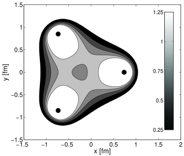
Figure 21: Energy density of the $qqq$ configuration. Black dots show particle positions. White voids at particles are spikes in the energy density due to the particles Coulomb peaks which are cut out. Upper left: $\epsilon_{\text{el}}$, upper right: $\epsilon_{\text{vol}}$, lower left: $\epsilon_{\text{sur}}$, lower right: $\epsilon_{\text{tot}}$. Lines are equidistant in energy density with the values given in the figures.

In figure 21 we show the energy density of the different types together with the total energy density obtained with parameter set PS-I for a $qqq$ state with quark separation $R=1.7\!$ fm. A clear difference in the geometries is seen for the different energy fraction. The electric energy distribution (upper left panel) shows pairwise electric flux tubes between the three quarks, bent into the center of the baryon. The geometry is nearly $\mathsf{\Delta}$-shaped due to the dip at the center. Going along the $x$-axis from the center into the negative direction, there is a well in the energy density of about $95\,$MeV/fm³, corresponding to 20% of the central value. This is qualitatively the same for all parameter sets, but the energy barrier is larger in PS-II ($120\,$MeV/fm³) and smaller in PS-III ($90\,$MeV/fm³).

In contrast to the electric part of the energy the volume part has a clear Y-shaped structure (upper right panel) which is the same as for the dielectric function $\kappa(\sigma)$ shown in figure 20. The surface part (lower left panel) is only relevant where $\sigma$ varies spatially. This is true on the edges of the triangle and one sees therefore a pure $\mathsf{\Delta}$-like distribution. The absolute value of the surface energy density in the flux tubes is small compared to the values in the electric and the volume fluxes.

The sum of all three energies results in the total energy density shown in the lower right panel. The picture shows qualitatively the same structure as the one for the electric energy. But the barrier of the total energy is only 10% of the central value and the competing structures of the electric energy and the volume energy are smeared out.

We will study now whether this picture of superimposed structures can be found in the baryonic potential when the size of the $qqq$ state is varied. The result is shown in figure 22 together with the Y and the $\mathsf{\Delta}$-parameterization of the Cornell potential (35).

Figure 22: The total energy of the $qqq$ state compared to the Y and the $\mathsf{\Delta}$-forms of the Cornell parameterization.

The absolute values of the total energy agree very nicely with the $\mathsf{\Delta}$-parameterization which is in line with the results in Bali (2001); Alexandrou et al. (2002a). However, it is the string tension $\tau_{qqq}$ that distinguishes the two parameterizations and not the absolute value $E_{\text{tot}}$. If one takes a closer look at the potential, one sees a slightly larger slope than expected from the $\mathsf{\Delta}$-picture. To analyze the baryon potential with respect to $\tau_{qqq}$ we make a fit of the form

$$V_{qqq}=3C_{F}^{\text{ab}}E_{0}-\frac{3}{2}C_{F}^{\text{ab}}\frac{\alpha}{R}+\tau_{qqq}R$$ (36)

to the CDM results and extract the string tension $\tau_{qqq}$ from the fit. Here $E_{0}$ and $\alpha$ are free fit parameters as well. As in the $q\bar{q}$ case we make this fit to the total energy (21a) as well as to the electric, the volume and the surface parts of the energy (21b)–(21d) to see if the different contributions show the same behavior as the energy distributions in figure 21.

	PS-I	PS-II	PS-III
$\tau_{qqq}$[MeV/fm]	1544	1568	1517
$\delta\tau$	0.33	0.41	0.21
$\tau_{qqq}^{\text{el}}$[MeV/fm]	616	588	607
$\delta\tau_{\text{el}}$	0.11	0.05	-0.29
$\tau_{qqq}^{\text{vol}}$[MeV/fm]	650	670	725
$\delta\tau_{\text{vol}}$	0.88	1.11	0.72
$\tau_{qqq}^{\text{sur}}$[MeV/fm]	278	311	184
$\delta\tau_{\text{sur}}$	-0.3	-0.016	0.01

Table 7: The $qqq$ string tension of the baryon Cornell potential and the deviation $\delta\tau$ from the expected Y ($\delta\tau=1$) and $\mathsf{\Delta}$-picture ($\delta\tau=0$).

The result of the fits is summarized in table 7. Here we show only the values for the $qqq$ string tension as both the constant term and the Coulomb term scale in the same way in the $\mathsf{\Delta}$ and the Y-geometry. Together with $\tau_{qqq}$ we show the deviation $\delta\tau=(\tau_{qqq}-\tau_{\mathsf{\Delta}})/(\tau_{\mathsf{Y}}-\tau_{\mathsf{\Delta}})$ from the expected values in both pictures. A value $\delta\tau=0\;(1)$ indicates perfect agreement with the $\mathsf{\Delta}\;(\mathsf{Y})$ picture whereas $\delta\tau\approx 0.5$ means that neither the Y nor the $\mathsf{\Delta}$ is realized but a transition between both geometries.

First we confirm the visual impression that the electric and the surface part of the string tension $\tau_{qqq}^{\text{el}}$ and $\tau_{qqq}^{\text{sur}}$ are well described by the $\mathsf{\Delta}$-picture. All deviations from the $\mathsf{\Delta}$ parameterization $\delta\tau$ are close to or even undershoot zero. In the surface part of PS-I this can be explained by the respective energy density (lower left panel in fig. 21). There most part of the energy is located outside the region defined by the triangle of the quarks. The opposite is true for the volume part $\tau_{qqq}^{\text{vol}}$. Here the deviations are close to one, indicating a better description by the Y-geometry. In the $qqq$ case the equality between the electric and the surface part of the string tension is not true anymore. For PS-III $\tau_{qqq}^{\text{vol}}$ is larger than $\tau_{qqq}^{\text{el}}$ by 20% with the same tendency in the other two parameter sets.

The total string tension $\tau_{qqq}$ as a superposition of the three parts takes on a value in between the $\mathsf{\Delta}$ and the Y-value. All parameter sets have a slight preference for the $\mathsf{\Delta}$-picture with parameters $\delta\tau$ between 0.21 (PS-III) and 0.41 (PS-II).

Another useful check for the scaling is to look at the $qqq$-potential for arbitrary geometry of the $qqq$-triangle. With the parameterizations for the Y and the $\mathsf{\Delta}$-picture one would expect a universal behavior of the long range part of the potential with the total string length $L$. For the Y-geometry we have $L_{\mathsf{Y}}=\sum_{i}|\vec{r}_{i}-\vec{r}_{c}|$ and for the $\mathsf{\Delta}$-geometry $L_{\mathsf{\Delta}}=\sum_{i<j}|\vec{r}_{i}-\vec{r}_{j}|$. For triangles with no angle exceeding $120^{\circ}$ the minimal string length $L_{\mathsf{Y}}$ can be calculated Bornyakov et al. (2004) with

$$L_{\mathsf{Y}}=\left(\frac{1}{2}\sum_{i<j}(\vec{r}_{i}-\vec{r}_{j})^{2}+2\sqrt{3}S_{\mathsf{\Delta}}\right)^{1/2}\quad,$$ (37)

where $S_{\mathsf{\Delta}}$ is the area of the triangle spanned by the three quarks.

Figure 23: The $qqq$-potential for arbitrary placed quarks as a function of the total string length $L_{\mathsf{Y}}$ and $L_{\mathsf{\Delta}}$ respectively. $L_{\mathsf{\Delta}}$ is scaled by a factor $1/\sqrt{3}$ and the corresponding potential is shifted by -0.5 GeV for better visibility.

We show in fig. 23 the $qqq$ potential for arbitrary quark positions. We have selected only those triangles, where all angles are smaller than $120^{\circ}$ and where the 2-particle distance $|\vec{r}_{i}-\vec{r}_{j}|>0.4\,$fm. The visual impression agrees with the previous result, that the $qqq$-potential is better described by the $\mathsf{\Delta}$-geometry. The potential plotted as a function of $L_{\mathsf{Y}}$ scatters more strongly in the energy than in the $\mathsf{\Delta}$-case where it follows a rather straight line. Note that this result is different to that obtained in Bornyakov et al. (2004).

In summary the $qqq$ configuration shows two competing geometries visible in the energy distribution and in the potential. The scalar field has a Y-like structure while the electric energy follows a $\mathsf{\Delta}$-like distribution. In the former case the bag energy is minimized by minimizing the volume of the three-quark bag. However, the flux tubes have a finite transverse extent with no sharp boundaries. Therefore the electric flux is not restricted to the Y-shaped flux tube but may evolve in a region outside the scalar Y-volume. The superposition of both the electric and the scalar energy distributions leads to a potential right in-between the two ansätze, which is qualitatively the same result as obtained in a lattice calculation Alexandrou et al. (2003).

VI Conclusions and Discussion

In this work we have shown that the Chromo Dielectric Model is able to describe confinement of overall color neutral systems by the formation of color flux tubes in a perfect dielectric vacuum. We studied the dependence of the string tension and the string profile on the model parameters. The parameters of the model were chosen carefully to reproduce the profile of $q\bar{q}$ strings as well as the $q\bar{q}$ potential obtained in lattice calculations and from heavy-meson spectroscopy. Three different parameter sets were found that describe the profile of the $q\bar{q}$ flux tube obtained on the lattice optimally under given constraints. All parameter sets reproduce the phenomenological value of the string tension $\tau=980\,$MeV/fm. Parameter set PS-I additionally describes both the width as well as the shape of the flux tube rather well. In PS-II we fixed the bag constant and the glueball mass parameters to values from the literature and found that only the width of the profile can be reproduced. The shape develops a steeper profile than the lattice profile. In a final set we have fixed as well the coupling constant to reproduce also the Coulomb parameter of the Cornell potential. With this parameter set PS-III the resulting string width is larger by 20% than the value obtained on the lattice. The profiles of the strings reach their asymptotic shapes for quark separations larger than $R=1.2\,$fm. However, the width does not saturate at a constant value but increases slowly, which is in line with the lattice expectation, where the string width increases logarithmically. It would be desirable if there were SU(3) lattice data available of the same accuracy as obtained within SU(2) lattice calculations. Then one could compare the CDM results to a somewhat more realistic theory.

We have also made a comparison of the $q\bar{q}$ flux tubes obtained in CDM to the calculations within the Dual Color Superconductor. We were able to extract a magnetic current in the CDM showing the same vortex-like behavior as in the DCS. Both the profile of the electric field and the magnetic current were in qualitative agreement with the profiles calculated within the Dual Color Superconductor model and also calculated on the lattice.

Finally we have shown that the $q\bar{q}$ string tension does not obey the Casimir scaling hypothesis. The scaling of the adjoint string tension with $\sqrt{C_{A}/C_{F}}$ and not with $C_{A}/C_{F}$ is a general feature of all bag-like models. Casimir scaling has not been proven unambiguously on the lattice and therefore does not exclude our model.

For $qqq$ configurations we have calculated the color electric fields, the color invariant energy density and the $qqq$ potential to discuss the geometric form of those baryonic states. We have found two competing pictures in the electric and the scalar part of the system. The scalar energy distribution is confined into a clear Y-like form whereas the electric energy distribution is of the $\mathsf{\Delta}$-type form. In the total energy the overall values are in good agreement with the $\mathsf{\Delta}$-type of the $qqq$ Cornell parameterization but the string tension $\tau_{qqq}$ shows the same competing behavior as the energy distributions: $\mathsf{\Delta}$-like in the electric sector and Y-like in the volume sector of the energy. The total string tension thus has neither the Y nor the $\mathsf{\Delta}$-like value but lies rather in-between the two pictures.

Out of the three parameter sets PS-I to PS-III the first one describes best all lattice data of $q\bar{q}$ flux tubes shown in the present work, although the values of the model parameters differ from that found in the literature. It should be noted, that the identification of $m_{g}$ with the glueball mass and of $B$ with the gluon condensate obtained in QCD sum rules is motivated from heuristic arguments only. Thus the results obtained with PS-I give a good agreement to lattice data and the other two serve for a comparison if the space of model parameters is restricted to the values given above. The Chromo Dielectric Model gives therefore an adequate mechanism of confinement, which can be understood dynamically.

It would be interesting to see the influence of the color electric fields within a self-consistent treatment including also the quarks dynamically. Those calculations were done in Wilets (1989) including a direct interaction between the confinement field and the quark field only. In our model the interaction with the quark field is only indirect via the quark-gluon interaction $-g_{s}\bar{\psi}\gamma_{\mu}t^{a}A_{a}^{\mu}\psi$ and the interaction of the gluons with the confinement field. Here $\psi$ is the quark field obeying the Dirac equation.

A natural extension of our calculations is to include also time-dependent fields according to eq. (18). Those studies were done in Traxler et al. (1999) where only the confinement field was treated dynamically. Within those time-dependent calculations one could study the hadronization out of a gas of colored quarks and gluon fields which might be produced in a relativistic heavy-ion collision. Hadronization is up to now treated as an instantaneous process at the freeze-out temperature. Within our model one could test this assumption as a time-resolved process. Of course this is numerical challenging due to the complexity of the equations but might be feasible within nowadays computing power.

Appendix A Numerics

A.1 The FAS-Algorithm

To solve the set of equations (22) we define a rectangular box with fixed volume $V=L_{x}\times L_{y}\times L_{z}=L^{3}$ and discretize the equations on a Cartesian grid $\Omega_{h}$ with $N=n^{3}$ nodes and $n=2^{m}=128$. The grid spacing is therefore $h=L/n$. The particle positions are not restricted to this grid, but can be placed arbitrary. To avoid spurious oscillations in observable quantities when changing the quark position, we assign a spatial width to the quarks given by $r_{0}$. For the grids used in this work with $L=3\,$fm we have a grid spacing $h\approx 0.02\,$fm and this determines the width $r_{0}=0.02\,$fm.

We use the Full Approximation Storage (FAS) multigrid algorithm described in Brandt (1982); Briggs (1987); Joppich (1991); Press et al. (1996). The FAS algorithm is especially suited for our purposes because both the needed memory resources and the computing time scale only with the number of grid points $N$ which is mandatory for those large systems. It is like any other multigrid algorithm an iterative solution technique that improves on an initial guess for the solution step by step. Conventional relaxation methods cease to converge for grids with increasing $n$ (decreasing $h$). This means that the convergence get worse if one wants to decrease the discretization error. To be more precise it is the low frequency part of the system which does not converge anymore. The grid introduces an infrared cutoff due to the finite dimensions $L$ of the box and an ultraviolet cutoff due to the finite number of grid points $n$ (known as Brillouin zone in solid state physics). The Fourier spectrum of the solution is built up of modes with wave vector $k_{i}=(\pi/L\ldots i\pi/L\ldots k_{\text{max}}=n\pi/L)$. Modes of the error made in approximating the true solution with wave vector $k_{i}$ and $i>n/2$ (oscillating modes) are damped out fast, but modes with $i<n/2$ (smooth modes) do not die out due to the locality of the difference operator.

To cure this problem the algorithm introduces temporary coarser grids $\Omega_{\ell}$ with $n_{\ell}=(n/2,n/4,\ldots,2^{-\ell}n,\ldots,2)$ nodes per dimension. On those grids the spectrum is reduced to modes with maximal wave vector $k_{\text{max}}^{\ell}=2^{-\ell}k_{\text{max}}$ and smooth modes on the fine grid become oscillating modes on the coarse grid. Further relaxation of the solution on the coarse grid allows to solve for those modes and in turn to get an estimate for the error made on the fine grid.

Thus the FAS algorithm consist of three building blocks: (i) the relaxation method on each grid, (ii) the transport of the approximation from a fine grid to the next coarser grid and (iii) the transport back from the coarse to the fine grid. The recursion starting from the finest grid $\Omega_{0}=\Omega_{h}$ down to the coarsest $\Omega_{m-1}$ and back is called a V-cycle. In contrast to linear multigrid algorithms the FAS algorithm allows also for non-linear differential equations.

Both the electric potentials $\phi^{a}$ and the confinement field $\sigma$ are solved within the same algorithm at once. As a smoothing method we use $\mu=4$ Gauss-Seidel relaxations with red-black ordering for the smoothing update on each grid both on the downward and the upward stroke of the V-cycle. For the discretized version of eq. (22b) we have to include a Newton–Raphson approximation in order to cope with the non-linearity. The transfer of all discretized field quantities from coarse to fine grids and back is performed with linear interpolation and full weighting reduction operators respectively. To improve the convergence of the algorithm we have to find a good initial guess to start the V-cycle on the finest grid $\Omega_{0}=\Omega_{h}$. To this end we first find a solution on the next coarser grid $\Omega_{1}$ which is much less expensive in the computational costs. In general we find a solution on every grid $\Omega_{\ell}$ with an initial guess found on the grid $\Omega_{\ell+1}$.

The computational costs of the multigrid V-cycle in $d$ space dimensions can be estimated as follows Briggs (1987). The $\gamma=3$ independent fields ($\sigma,\phi^{a})$ and the corresponding residuals defined below in eqs. (38) are stored on a grid with $n^{d}$ nodes. Thus the minimal amount of memory needed is given by $M_{1}=m_{1}\gamma n^{d}$ float value units with $m_{1}=2$. On each of the $n^{d}$ nodes the discretized equations for the $\gamma$ fields are solved locally $2\mu$ times and the $\gamma$ residuals are calculated once. If we estimate the amount of work for the transfer between the fine and the coarse grid with another $2n^{d}$ operations, the minimal number of computational operations on each grid is given by $M_{2}=(2\mu+3)\gamma n^{d}=m_{2}\gamma n^{d}$ with $m_{2}=11$. We may call the minimal amount of memory $M_{1}$ and the minimal number of numerical operations $M_{2}$ one memory unit and one working unit respectively. The equivalent numbers on a coarse grid $\Omega_{\ell}$ are $M_{1/2}^{\ell}=m_{1/2}\gamma(n/2^{\ell})^{d}$. An upper limit for the numerical costs summed over all coarse grids can be estimated by a geometrical series $\sum_{\ell=0}^{\infty}M_{1/2}^{\ell}=m_{1/2}\gamma n^{d}(1-2^{d})^{-1}=\frac{8}{7}m_{1/2}\gamma n^{d}$ for $d=3$. The algorithm is surprisingly more efficient in higher dimensions $d$. In $d=3$ space dimensions the amount of memory needed is therefore only $\frac{8}{7}m_{1}$ times larger than that for traditional relaxation methods and the computational work for a whole V-cycle sums up to $\frac{8}{7}m_{2}$ times that for one relaxation sweep. One sees that the total computational costs scale only linearly with the number $\gamma n^{d}$ unknowns.

We impose Dirichlet boundary conditions on the confinement field $\sigma=\sigma_{\text{vac}}$ and von-Neumann boundary conditions on the electric potentials, i.e. $\frac{\partial\phi^{a}}{\partial n}=0$ where $\vec{n}$ is a normal vector to the boundary. This forbids any electric flux out of the computational domain and is in line with the observed fact, that the electric flux is compelled into the flux tube.

We compute after each V-cycle the residuals

$$r_{\phi}^{a} = \nabla\cdot(\kappa(\widetilde{\sigma})\vec{\nabla}\widetilde{\phi}^{a})+g_{s}\rho^{a}$$ (38a)

$$r_{\sigma} = \nabla^{2}\widetilde{\sigma}-U^{\prime}(\widetilde{\sigma})+\kappa^{\prime}(\widetilde{\sigma})\vec{\widetilde{E}}^{a}\cdot\vec{\widetilde{E}}^{a}\quad.$$ (38b)

with the approximations $\widetilde{\phi}^{a}$ and $\widetilde{\sigma}$ and the corresponding energies given in eq. (21). We observe a rapid decrease of $|r_{\phi}|$ and $|r_{\sigma}|$ and simultaneously a fast convergence to the asymptotic values of the energy. We show as an example $r_{\sigma}$ and $E_{\text{tot}}$ as a function of the computational work in figure 24 for the multigrid algorithm (solid symbols) and for pure Gauss-Seidel relaxation (open symbols). For both methods we have started with the same initial guess obtained on the next coarser grid.

Figure 24: The residual $r_{\sigma}$ (left) and the total energy (right) as a function of the number of V-cycles in the FAS algorithm. Gauss–Seidel relaxation are the open symbols, the FAS results are given with solid symbols. Note the logarithmic scale for the computational work.

On the left panel one sees, that the rate of convergence is slowing down for Gauss-Seidel relaxation when going from small grids ($n=32$) to larger grids ($n=128$) whereas it is independent of the discretization within the FAS algorithm. On the right panel we see that the total energy converges very rapidly to the asymptotic one in the FAS algorithm. In practice we stop the algorithm if the total energy stays constant within a given error of $10^{-3}$. This is reached usually after three to five V-cycles on the largest grid. The time needed for the solution is reduced by nearly 2 orders of magnitude as compared to ordinary relaxation. On a 2.2 GHz Pentium 4 machine a typical configuration is solved on a ($N=128^{3}$) grid within 5-6 minutes.

A.2 The vacuum value of the dielectric constant

In the spirit of the model one should set $\kappa_{\text{vac}}=0$. However the Poisson eq. (22a) is ill-defined in the perturbative phase in this limit. In Bickeboeller et al. (1985) it was shown that in order to get a consistent solution for the flux tube, one also must have $\kappa^{\prime}(\sigma_{\text{vac}})=0$. Therefore we have parameterized the dielectric constant according to eqs. (10) and (17) with a finite but small value for $\kappa_{\text{vac}}$. With this form also $\kappa^{\prime}(\sigma_{\text{vac}})\rightarrow 0$ for $\kappa_{\text{vac}}\rightarrow 0$. As we are dealing with a boundary value problem we could not start right away with $\kappa^{\prime}(\sigma_{\text{vac}})=0$ as in this limit $\sigma=\sigma_{\text{vac}}$ everywhere is a solution of (22b) which will be found by the algorithm. Therefore we have chosen a rather large value $\kappa_{\text{vac}}=10^{-2}$ when finding an initial guess on coarser grids with $n\leq 32$. We then decrease the value of $\kappa_{\text{vac}}$ step by step on the finer grids until a prescribed minimal value is reached. We have analyzed the dependence of the string quantities on $\kappa_{\text{vac}}$. In fig. 25 we show that the string tension as well as the profile parameters do not depend on $\kappa_{\text{vac}}$, once it is smaller than say $\kappa_{\text{vac}}=10^{-3}$. The numerics were still stable and fast for $\kappa_{\text{vac}}=10^{-4}$ which we have used throughout this work. Of course it is not possible to calculate the energy of a single-quark configuration, as the radius of the bag diverges and most of the electric energy is stored outside the bag. But we can estimate this energy in the same spirit as for the cylindrical flux tube with sharp boundaries in eq. (29) and obtain $E_{q}=\frac{1}{3}[(2g_{s}^{2}C_{F}B)/(\pi^{2}\kappa_{\text{vac}}^{3})]^{1/4}$. With the smallest values used in our model ($B^{1/4}=240\,$MeV and $g_{s}=2$) we obtain $E_{q}=66\,$GeV which is large on a hadronic scale.

Figure 25: All parts of the string tension (left) and parameters defining the shape of the profile (right) saturate very fast for decreasing values of $\kappa_{\text{vac}}$. In all results shown in this work, we have used a value $\kappa_{\text{vac}}=10^{-4}$.