Theoretical Implications of the LEP Higgs Search

Abstract

We study the implications for the minimal supersymmetric standard model (MSSM) of the absence of a direct discovery of a Higgs boson at LEP. First we exhibit 15 physically different ways in which one or more Higgs bosons lighter than the LEP limit could still exist. For each of these cases – as well as the case that the lightest Higgs eigenstate is at, or slightly above, the current LEP limit – we provide explicit sample configurations of the Higgs sector as well as the soft supersymmetry breaking Lagrangian parameters necessary to generate these outcomes. We argue that all of the cases seem fine-tuned, with the least fine-tuned outcome being that with $m_{h}\simeq 115~{}\mathrm{GeV}$. Seeking to minimize this tuning we investigate ways in which the “maximal-mixing” scenario with large top-quark trilinear A-term can be obtained from simple string-inspired supergravity models. We find these obvious approaches lead to heavy gauginos and/or problematic low-energy phenomenology with minimal improvement in fine-tuning.

The Minimal Supersymmetric Standard Model is defined as the simplest supersymmetric extension of the Standard Model (SM). Every SM particle has a superpartner, the basic Lagrangian is supersymmetric, and the gauge group is the same $SU(3)\times SU(2)\times U(1)$ as that of the SM. The full supersymmetry is softly broken by certain dimension two and three operators. There is considerable indirect evidence that this theory is likely to be part of the description of nature. If it is, a Higgs boson with mass less than about $130~{}\mathrm{GeV}$ must exist, and superpartners must be found with masses not too much larger than those of the W, Z and top quark. While the Higgs boson mass can be as heavy as $130~{}\mathrm{GeV}$ in the MSSM, it has been known for some time that most naive models imply a lighter state, usually below about $110~{}\mathrm{GeV}$, when constraints from non-observation of superpartners (real or virtual) are imposed, and including the constraint that the indirect arguments for supersymmetry are valid without fine-tuning.

While it is not impossible that perhaps LEP has seen a Higgs boson with $m_{h}\simeq 115~{}\mathrm{GeV}$, the data collected up through center-of-mass energy of $209~{}\mathrm{GeV}$ LHWG01 yields no unambiguous signal for such a light Higgs eigenstate. One obvious explanation for this fact is that the lightest Higgs boson is heavier than $115~{}\mathrm{GeV}$. Another is that one or more eigenstates are lighter than the kinematic cut-off but that they do not couple significantly to the Z-boson. Thus it is natural to ask whether the Higgs sector of the MSSM could be such that LEP would not have found a signal because of reduced Higgs cross sections or reduced branching ratios in some part of the general MSSM parameter space. Using the reported LEP limits on the cross-section $\times$ branching ratio for Higgs eigenstates as a guide, it is possible to find 15 logically distinct ways in which this could indeed have been the case at LEP. Together with the possibility that the lightest Higgs boson is at $115~{}\mathrm{GeV}$, and the possibility that it is much larger in mass, there are 17 distinct configurations of the MSSM Higgs sector consistent with the LEP results. These cases are summarized in Table 1 of Section II below, with an explicit example configuration for each case given in Table 2. The results in Table 1 are not the outcome of a complete parameter scan, but instead represent a general classification of logical possibilities for the MSSM Higgs sector. All of our example points allowed by other data. All satisfy the constraints for electroweak symmetry breaking, though sometimes in unconventional ways. All of the example configurations are detectable at the Fermilab Tevatron collider with sufficient luminosity. If the MSSM is the correct description of nature just above the electroweak scale then one of these 17 cases is the true Higgs sector of the MSSM.

In Section I we review the data collected at LEP, with particular attention paid to what is strictly measured and how these measurements are converted into limits on Higgs eigenstate masses. As mentioned above, there is no clear indication for the presence of Higgs bosons in the LEP data. Nevertheless there are three distinct cases where an excess of observed events in a particular channel resulted in an experimental bound on the cross section $\times$ branching ratio that was weaker than the expected limit at the $2\sigma$ level LHWG02 ; LHWG03 ; So02a ; So02b . In these “excess regions” care must be taken in extracting a mass bound on the possible Higgs eigenstates involved. Using these regions as a guide we classify the possible consistent Higgs configurations in Section II. In that section we provide a general description of each of the 17 logically distinct cases as well as a concrete example configuration to illustrate each case.

With these 17 cases in hand it is natural to then ask whether any of them are less fine-tuned than the others, and thus might be more likely to point to a particular underlying theory. To address this issue it is necessary to construct a soft supersymmetry breaking Lagrangian capable of giving rise to each of the 17 possible configurations. Since not all 105 parameters of the MSSM are relevant for determining the Higgs sector of the theory, there is some inevitable arbitrariness in this construction. It is for this reason that LEP results are often interpreted in the light of certain “benchmark” models to reduce this arbitrariness. We have chosen to work in a less restrictive environment and provide candidate soft Lagrangian parameters at both the electroweak scale and the high-energy (in this case GUT) scale in Section III. Interestingly, only 4 of the 17 cases can be obtained from a model such as minimal supergravity (mSUGRA) with a universal gaugino mass, universal scalar mass and universal soft trilinear coupling at the GUT scale. This includes the cases where the lightest Higgs boson is at, or much larger than, $115~{}\mathrm{GeV}$. Despite the 15 distinct ways the Higgs could have been lighter than $115~{}\mathrm{GeV}$ and escaped detection, the most natural conclusion within the MSSM is still that the Higgs is at, or just slightly above, 115 GeV in mass. This conclusion is arrived at in Section III through a variety of means: investigating the low energy parameter space, examining the high energy soft Lagrangian as well as a fine-tuning analysis using the sensitivity parameters of Barbieri and Giudice BaGi88 .

Achieving such a large Higgs mass in the MSSM will necessitate at least some level of uncomfortable tuning because the tree level Higgs mass is bounded by $M_{Z}$ and thus the one loop corrections have to supply about $\delta m^{2}_{h}\simeq(70~{}\mathrm{GeV})^{2}$ when added in quadrature. This tuning is most mitigated in the so-called “maximal-mixing” regime, which implies a very large soft trilinear coupling involving the stop and where the gluino can be made as light as possible. While widely used as a benchmark case in low-energy studies of the Higgs sector of SUSY models, such a regime does not seem to be a robust outcome of any of the standard SUSY breaking/transmission models typically considered in the literature. We study the general improvement in fine-tuning when maximal-mixing in the stop sector is obtained in Section IV. In Section V we focus on string-based models and look at ways to engineer such large mixing in the stop sector. We find that the most obvious ways to approach maximal mixing result in either heavy gauginos or a problematic low energy phenomenology. Thus explaining the LEP result without excessive tuning in these simple models seems difficult. We conclude with some speculation on how extending these string-based models in theoretically well-motivated directions could alleviate the problem.

I Overview of the LEP Results

In order to appreciate the theoretical implication of the LEP Higgs search on high energy models it is necessary to understand the way in which data is collected and interpreted by the LEP experimental collaborations. This, in turn, requires a brief review of the salient features of the Higgs sector in the MSSM. In this section we aim to provide sufficient background to motivate the classification scheme for low-energy models adopted in Section II.

I.1 What is measured at LEP

There are three neutral Higgs states in the MSSM. If there is no CP violating phases then these neutral Higgs mass eigenstates are also CP eigenstates: two of them are CP-even and one is CP-odd. If Higgs bosons are produced at LEP then the relevant process will be $e^{+}e^{-}\to Z^{*}\to\phi_{i}Z$ or $e^{+}e^{-}\to Z^{*}\to\phi_{i}\phi_{j}$, where $\phi_{i}$ represents any of the three neutral Higgs mass eigenstates. It is therefore convenient to define the following Higgs/Z-boson couplings

$$ZZ\phi_{i}:\;\frac{g_{2}m_{Z}}{\cos\theta_{W}}C_{i}\quad\mbox{and}\quad Z\phi_{i}\phi_{j}:\;\frac{g_{2}}{2\cos\theta_{W}}C_{ij}.$$ (1)

Since the Standard Model Higgs boson has the coupling $ZZH_{\mathsc{sm}}:\;g_{2}m_{Z}/\cos\theta_{W}$, the $C_{i}$’s are to be interpreted as ratios of the true couplings to those of the SM. When CP is conserved we may use $h$, $H$ and $A$ to denote the lighter CP-even, heavier CP-even and CP-odd Higgs states, respectively. In this CP-conserving case only $C_{h}$, $C_{H}$, $C_{hA}$ and $C_{HA}$ are non-zero and we have the relations

$$|C_{h}|^{2}+|C_{H}|^{2}=1\;;\qquad C_{hA}=C_{H}.$$ (2)

The $C_{i}$ can be related to the Higgs mixing angle $\alpha$ and the ratio of the vevs of the up-type to down-type Higgs field defined by $\tan\beta=v_{u}/v_{d}$. For example, in the CP-conserving case the one independent variable can be written as $C_{h}=\sin(\beta-\alpha)$. In addition to the proportionality factor $C_{ij}$, when a CP-even Higgs boson is produced in association with the CP-odd state there is a kinematic p-wave suppression factor $\bar{\lambda}$ such that $\sigma(e^{+}e^{-}\to A\phi_{i})\propto\bar{\lambda}\sigma_{\mathsc{sm}}$ where

$$\bar{\lambda}=\frac{\lambda_{A\phi_{i}}^{3/2}}{\lambda_{Z\phi_{i}}^{1/2}(12m_{Z}^{2}/s+\lambda_{Z\phi_{i}})}\;;\;\lambda_{ij}=\frac{1-(m_{i}+m_{j})^{2}/s}{1-(m_{i}-m_{j})^{2}/s}.$$ (3)

All of these proportionality factors are model-dependent, as are the masses of the various Higgs eigenstates.

Once produced, Higgs eigenstates are identified through their decay products. In most of the MSSM parameter space the three neutral Higgs eigenstates decay predominantly into the heaviest accessible fermion – typically either a $b,\bar{b}$ or $\tau^{+},\tau^{-}$ pair. In some areas of parameter space decays into other quark/antiquark pairs are important, particularly to charm quarks. In still other regions of the MSSM parameter space a heavy Higgs eigenstate may decay into lighter eigenstates (though only in the presence of CP violation) and/or decay into light neutralinos which can escape the detector. We shall refer to the latter case as an “invisible decay,” though such event signatures can be and have been analyzed at LEP.

In both production processes $Z\phi_{i}$ and $\phi_{i}\phi_{j}$, a crucial element in reconstructing the event as one involving a Higgs eigenstate is the reconstruction of the associated partner – whether it be a Z-boson or another Higgs eigenstate. Thus the most important category of event signature is a four-jet event, with both the Higgs eigenstate and the associated production partner decaying into quark/anti-quark pairs. To reduce the background from processes such as $e^{+}e^{-}\to ZZ,W^{+}W^{-}$ b-tagging is typically used to require that at least one pair of jets arise from a $b,\bar{b}$ pair. As the Higgs states tend to decay to b quarks more frequently than Standard Model gauge bosons, this data set will tend to have a larger proportion of Higgs events.

Thus we might crudely think of classifying events at LEP in terms of a set of topologies. Some of these topologies, such as $b\bar{b}\ell^{+}\ell^{-}$ (with $\ell^{\pm}$ either an electron or a muon) , are more likely to come from the process $e^{+}e^{-}\to Z\phi_{i}$ than from $e^{+}e^{-}\to\phi_{i}\phi_{j}$. Others, such as $b\bar{b}\tau^{+}\tau^{-}$, may fit quite well with either production mechanism. To account for this ambiguity, each event that passes the initial cuts is assigned a measure of its “signal-like” properties under the hypothesis of the process $e^{+}e^{-}\to Z\phi_{i}$ and the process $e^{+}e^{-}\to\phi_{i}\phi_{j}$. An event where the invariant mass of a lepton pair closely matches the Z-boson mass, for example, will then be more “signal-like” under the former hypothesis than under the latter. This weight is a function not only of the experimentally reconstructed Higgs mass for the state $\phi_{i}$ but also of the true Higgs mass $m_{\phi_{i}}$ for that state. Thus asking whether a given event “looks like a Higgs event” is complicated by the need to ask this question only in the context of a given hypothesis about how this Higgs state was created and what its true mass is. Equally challenging is asking the question of how many events of a given topology LEP should have seen for a given Higgs mass. What’s more, the likelihood that a particular event represents a signal is model-dependent, and will vary depending on whether we assume CP is conserved in the Higgs sector, or whether we assume a certain hierarchy of Higgs masses among the eigenstates.

It is therefore more useful to think of a limit on the production cross-section $\times$ branching ratio for the process $e^{+}e^{-}\to Z\phi_{i}$ and the process $e^{+}e^{-}\to\phi_{i}\phi_{j}$ as a function of the Higgs eigenstate masses involved, bearing in mind that this limit will contain some residual model dependence. Since the Standard model production rate is known for a given Higgs mass $m_{\phi_{i}}$, we can normalize the limit to this quantity (and the known Z-boson branching ratios) to obtain the parameter $\xi^{2}$ reported by LEP

$$\xi^{2}_{Z\phi_{i}} = C_{i}^{2}\;{\rm Br}(\phi_{i}\to f\bar{f})/{\rm Br}(H^{\mathsc{sm}}\to f\bar{f})$$ (4)

$$\xi^{2}_{A\phi_{i}} = C_{Ai}^{2}\;\bar{\lambda}\;{\rm Br}(A\to f\bar{f})\;{\rm Br}(\phi_{i}\to f\bar{f}).$$ (5)

For each of the two production mechanisms, and each of the final state signatures, the effective number of events observed at LEP can be translated into a limit on the effective coupling $\xi^{2}$ for a given Higgs mass $m_{\phi_{i}}$.

Deciding whether a given point in the MSSM parameter space is “ruled out” by the LEP data is then more involved than simply calculating the masses of the Higgs eigenstates. Of key importance is the expected limit on $\xi^{2}$ for a particular channel. This is the bound that would be placed if all observed events that received some non-zero weight as “signal” events were in fact merely Standard Model background events. While the actual bound obtained by the LEP collaborations is consistent with this expected bound, there are three distinct excesses where the experimentally obtained bound was weaker than the expectation by approximately $2\sigma$ LHWG02 ; LHWG03 ; So02a ; So02b . The most celebrated of these is in the channel $e^{+}e^{-}\to Zh$ which shows an excess around $m_{h}\simeq 115~{}\mathrm{GeV}$. The two others occur in the channel $e^{+}e^{-}\to Zh$ with $m_{h}\simeq 98~{}\mathrm{GeV}$ and in the channel $e^{+}e^{-}\to Ah$ with $m_{h}+m_{A}=187~{}\mathrm{GeV}$. Any MSSM model that yields a Higgs configuration near one of these areas is governed by constraints from LEP that are quite different from those that yield a Higgs sector far from these areas.

I.2 How are mass limits obtained at LEP

The relative couplings given by the $C_{i}$ in (1) are functions of the Higgs mass spectrum. Thus, limits on the effective couplings $\xi^{2}$ can be translated into limits on these masses. The Higgs mass spectrum, in the CP-conserving limit, is determined at tree level by just two input parameters at the electroweak scale. These could be two eigenstate masses such as $m_{h}$ and $m_{A}$, or two angles such as the Higgs mixing angle $\alpha$ and the ratio of Higgs vevs given by $\tan\beta$, or some combination of the two. Note that these electroweak scale inputs are derived quantities and are not fundamental from the high-energy, underlying theory point of view.

At the loop level the Higgs mass spectrum requires several more inputs from the soft supersymmetry-breaking Lagrangian. Among these are the running squark masses for the third generation left-handed doublet $m_{\widetilde{Q}_{3}}^{2}=m_{\tilde{t}_{L}}^{2}=m_{\tilde{b}_{L}}^{2}$ and the right-handed third generation singlets $m_{\tilde{t}_{R}}^{2}$ and $m_{\tilde{b}_{R}}^{2}$, the trilinear scalar couplings associated with the top quark Yukawa $A_{t}$ and bottom quark Yukawa $A_{b}$, and the (supersymmetric) Higgs bilinear coupling $\mu$. At the next order the gluino mass is also important, not only in determining the Higgs mass spectrum but also for its contribution to the bottom quark Yukawa coupling which determines the Higgs branching fraction to $b,\bar{b}$ pairs. If we allow for CP violation in the Higgs sector we will also involve the relative phase between $\mu$ and $A_{t}$, which affects the masses of the various Higgs states as well as their couplings to the Z-boson.

In the presence of a CP violating phase (for example, the relative phase $\phi_{A\mu}$ between the $\mu$ parameter and the soft supersymmetry breaking trilinear coupling of the top squark) the mass matrix for the neutral Higgs states is a $3\times 3$ matrix. In the basis $\{{\rm Re}(h_{d})-v_{d},\;{\rm Re}(h_{u})-v_{u},\;\sin\beta\;{\rm Im}(h_{d})+\cos\beta\;{\rm Im}(h_{u})\}$ this is given by

$$M^{2}=\left(\begin{array}[]{ccc}m_{Z}^{2}\cos^{2}{\beta}+\widetilde{m}_{A}^{2}\sin^{2}{\beta}+\widetilde{\lambda}\Delta_{11}&-(\widetilde{m}_{A}^{2}+m_{Z}^{2})\sin{\beta}\cos{\beta}+\widetilde{\lambda}\Delta_{12}&r\widetilde{\lambda}\Delta\\ -(\widetilde{m}_{A}^{2}+m_{Z}^{2})\sin{\beta}\cos{\beta}+\widetilde{\lambda}\Delta_{12}&m_{Z}^{2}\sin^{2}{\beta}+\widetilde{m}_{A}^{2}\cos^{2}{\beta}+\widetilde{\lambda}\Delta_{22}&s\widetilde{\lambda}\Delta\\ r\widetilde{\lambda}\Delta&s\widetilde{\lambda}\Delta&\widetilde{m}_{A}^{2}+\widetilde{\lambda}\Delta\end{array}\right)$$ (6)

where $\widetilde{\lambda}=3\lambda_{t}^{2}/16\pi^{2}$ De99 . The mass $\widetilde{m}_{A}^{2}$ is proportional to the tree level value $m_{A}^{2}$ of the CP conserving case and reduces to it in the limit of $\phi_{A\mu}\to 0$. We have chosen to use the pair $m_{A}$ and $\tan\beta$ as our tree level input variables for the moment. The quantities $\Delta_{ij}$ represent radiative corrections to the tree level values of the CP even subsector. Explicit expressions for these quantities can be found in ElRiZw91 ; CaEsQuWa95 ; CaQuWa96 ; HaHeHo97 . The quantity $\Delta$ represents radiative corrections that are only present in the case of CP violation. Its value, as well as the dimensionless proportionality factors $r$ and $s$, can be found in De99 .

When we neglect the LR entries of the squark mass matrix (which is the case of “minimal mixing”), we have the following leading radiative corrections

$$\Delta_{11}=2\left(\frac{\lambda_{b}}{\lambda_{t}}\right)^{2}m_{b}^{2}\ln\frac{m_{\tilde{b}_{1}}^{2}m_{\tilde{b}_{2}}^{2}}{m_{b}^{4}}\;;\quad\Delta_{22}=2m_{t}^{2}\ln\frac{m_{\tilde{t}_{1}}^{2}m_{\tilde{t}_{2}}^{2}}{m_{t}^{4}}$$

$$r\Delta=0\;;\quad s\Delta=\frac{\sin\phi_{A\mu}}{\sin\beta}\frac{|\mu||A_{t}|m_{t}^{2}}{(m_{\tilde{t}_{2}}^{2}-m_{\tilde{t}_{1}}^{2})}\ln\frac{m_{\tilde{t}_{2}}^{2}}{m_{\tilde{t}_{1}}^{2}}$$ (7)

and $\Delta_{12}=0$. Note that the sizes of $\Delta_{11}$ and $\Delta_{22}$ are quite different: even in the large $\tan\beta$ regime, where $\lambda_{t}\sim\lambda_{b}$, the ratio $\Delta_{22}/\Delta_{11}\simeq 400$. Given that the one-loop correction $\Delta_{22}$ from the stop sector has a typical size on the order of $30~{}\mathrm{GeV}$, it follows that the one-loop correction $\Delta_{11}$ from the scalar bottom sector has a typical size $\Delta_{11}\sim 0.1~{}\mathrm{GeV}$ and is therefore negligible.

A particularly simple form for the above matrix which is often assumed is obtained under the assumptions that (i) there is no CP violation (ii) the tree level off-diagonal entries in (6) can be ignored and that (iii) $m_{A}\sin\beta\gg m_{Z}\cos\beta$. Then the approximate mass eigenvalues are $m_{A}^{2}$, $m_{H}^{2}=m_{A}^{2}\sin^{2}\beta$ and $m^{2}_{h}=m_{Z}^{2}\sin^{2}\beta+m_{A}^{2}\cos^{2}\beta+\widetilde{\lambda}m_{t}^{2}\ln[(m_{\tilde{t}_{1}}^{2}m_{\tilde{t}_{2}}^{2})/m_{t}^{4}]$. A more useful approximation to the lightest CP-even Higgs mass is obtained when the stop left-right mixing is restored. In this case the appropriate expression in the large $\tan\beta$ limit is $m_{h}^{2}\simeq m_{Z}^{2}+\delta_{h}^{2}$ where

$$\delta_{h}^{2}=\frac{3g^{2}m_{t}^{4}}{8\pi^{2}m_{W}^{2}}\left[\ln\left(\frac{m_{\tilde{t}_{1}}m_{\tilde{t}_{2}}}{m_{t}^{2}}\right)+X_{t}^{2}\left(1-\frac{X_{t}^{2}}{12}\right)\right].$$ (8)

The additional contributions from the second term in (8) are maximized for particular values of the stop mixing parameter $X_{t}\equiv(A_{t}-\mu\cot\beta)/M_{\mathsc{susy}}$. This property has been used to define the so-called “$m_{h^{0}}$-max” scenario CaHeWaWe99 which generates the maximum possible Higgs mass for a given value of $\tan\beta$ and typical Higgs mass. We will refer to this regime by its more common (though misleading) name of the “maximal mixing” scenario. The specific point defined in CaHeWaWe99 is given by the following combination of parameters:

$$\left\{\begin{array}[]{c}m_{\tilde{t}_{L}}=m_{\tilde{b}_{L}}=m_{\tilde{t}_{R}}=m_{\tilde{b}_{R}}\equiv M_{\mathsc{susy}}=1~{}\mathrm{TeV}\\ \mu=-200~{}\mathrm{GeV},\quad X_{t}\equiv(A_{t}-\mu\cot\beta)/M_{\mathsc{susy}}=2\\ M_{2}=200~{}\mathrm{GeV},\quad M_{\tilde{g}}=800~{}\mathrm{GeV},\quad A_{b}=A_{t}\end{array}\right\}$$ (9)

and the value of $\tan\beta$ restricted to lie in the range $0.4<\tan\beta<50$. Within this paradigm, the constraints on the various $\xi^{2}$ can be translated into the limits displayed in Figure 1 for the $(m_{h^{0}},m_{A})$ plane LHWG01 . The 95 % exclusion contour is represented by the dashed line in Figure 1: combinations of $m_{h}$ and $m_{A}$ above and to the left of this line would require a coupling $\xi^{2}$ for some process excluded at the 95% confidence level. In other words, within the context of the “$m_{h^{0}}$-max” scenario these combinations would have produced too many signal-like events at LEP. The utility of the $m_{h^{0}}$-max scenario is that the limits on the Standard Model-like Higgs eigenstate of the MSSM are the most conservative possible. It must be remembered, however, that the limits, the confidence level regions and the theoretically excluded areas will all change if the $m_{h^{0}}$-max scenario is replaced with a different interpretive paradigm.

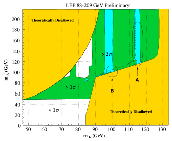
Figure 1: Distribution of confidence level in the $(m_{h},m_{A})$ plane for the $m_{h}^{0}$-max scenario LHWG01 . The white area marked $<1\sigma$ the observed number of events shows a deficit or is less than $1\sigma$ above the background prediction for this scenario. Similarly, the green shaded region marked $>1\sigma$ and the blue shaded region marked $>2\sigma$ showed an excess of observed events above the Standard Model background over $1\sigma$ and $2\sigma$, respectively. The 95% confidence level exclusion contour is given by the dashed line – points to the left of this line are excluded. We have highlighted two areas of particular interest: one centered around $m_{h}=114~{}\mathrm{GeV}$ (A) and one centered around $m_{h}=98~{}\mathrm{GeV}$ (B).

II Low-Energy Classification

We have learned from the preceding section that one can identify three distinct $2\sigma$ excesses in the LEP data consistent with the hypothesis that one or more Higgs eigenstates is produced. These correspond to the production of a (mostly) CP-even eigenstate of mass $98~{}\mathrm{GeV}$ and/or $115~{}\mathrm{GeV}$, as well as the production of two Higgs eigenstates with one being (mostly) CP-odd. By “mostly” we mean that in the presence of CP violating effects in the Higgs sector the wavefunction for the state in question is dominated by the component with the appropriate CP quantum number. We will see below that some interpretations of these excesses will require a degree of CP violation.

For the remainder of this section we will refer to these as $2\sigma$ “signals,” bearing in mind that some or all of these excesses may be simply the result of fluctuations in the background rate. Logically speaking, one can divide the MSSM parameter space into classes capable of producing one, two or three signals – as well as a much larger class that would give rise to no excess events at all. Given that properly applying the LEP constraints on Higgs masses depends on whether those masses fall near one of these excess regions, we believe this is a useful system for classifying possible MSSM models.

In all we find seventeen physically distinct scenarios compatible with the LEP results. In fifteen cases the lightest Higgs mass is kinematically accessible at LEP II but no signal is produced due to a reduction in the production cross section and/or branching ratios to bottom quarks. In addition there is the case where the lightest Higgs eigenstate is indeed Standard Model like with a mass $m_{h}=115~{}\mathrm{GeV}$ (No. 10) and the case where it is heavier than about 115 GeV (No. 17). These different configurations are summarized in Table 1.

Table 1: Possible explanations consistent with LEP Higgs search results. Ranges of neutral and charged Higgs masses consistent with background only hypotheses as well as one, two or three “signal” hypotheses are listed. The column headed by “Signals” indicates what signals might have appeared for a given model. Qualitative $\tan\beta$ and Higgs coupling ranges for each individual parameter space is given. All ranges should be understood as indicative of the allowed region at the roughly 10% accuracy level: fine scans of the parameter space have not been performed. For Higgs state $\varphi_{i}$ the $ZZ\varphi_{i}$ coupling is $(g_{2}M_{Z}/\cos\theta_{W})C_{i}$, approximate values are given in the table. The column marked $\phi$ indicates a non-trivial phase $\phi_{\mu A_{t}}$ is needed. When there is nontrivial phase, $m_{A}$ is understood as the mass of the neutral Higgs with smallest $C_{ZZH_{i}}$ coupling. The column $\mu$ indicates the presence of a large $\mu$ term. The column marked U indicates this scenario is compatible with a unified SUSY breaking scenario such as mSUGRA. We believe all other such scenarios effectively reduce to one of these.

No.	$m_{h}$	$m_{A}$	$m_{H}$	$m_{H^{\pm}}$	Signals	$\tan\beta$	$C^{2}_{h}$	$C^{2}_{H}$	U	$\mu$	$\phi$
1	98	89	115	112-123	98,115,187	6-12	0.2	0.8		Y	Y
2	98	$<m_{h}$	115	106-127	98,115	4-13	0.2	0.8		Y	Y
3	98	$\approx m_{h}$	115	121-136	98,115	5-50	0.2	0.8
4	98	115-130	115	112-124	98,115	10-24	0.2	0.8		Y
5	70-91	96-116	115	110-140	115,187	10-50	0.0	1.0		Y
6	98	89	$>115$	118-127	98,187	6-10	0.2	0.8		Y	Y
7	82-110	$<m_{h}$	115	$\sim m_{A}$	115	7-50	0.0	1.0		Y	Y
8	82-110	$\approx m_{h}$	115	$\sim m_{A}$	$115^{c}$	5-50	0.0	1.0	Y
9	82-110	115-140	115	$\sim m_{A}$	115	6-24	0.0	1.0		Y
10	115	$m_{A}\approx m_{H}>115$		$\sim m_{A}$	$115^{c}$	3-50	1.0	0.0	Y
11	98	100-130	120-130	$\sim m_{A}$	98	5-50	0.20	0.80
12	98	$<98$	120-130	106-128	98	4-13	0.20	0.80		Y	Y
13	65-93	94-120	116-125	110-140	187	8-50	0.0	1.0		Y
14	80-100	25-40	133-154	109-130	Nonea	2-5	0.5-0.8	0.2-0.5		Y	Y
15	111-114.4	$m_{A}\approx m_{H}>114.4$		$\sim m_{A}$	Noneb	2.1-4	1.0	0.0
16	70-114.4	90-140	$>114.4$	$\sim m_{A}$	None	4-50	0.0	1.0	Y
17	$>114.4$	$m_{A}\approx m_{H}>114.4$		$\sim m_{A}$	Nonec	4-50	1.0	0.0	Y

^a Dominant decay is CP violating process $H_{2}\to H_{1}H_{1}$. This case was studied in Ref. CaElPiWa00, .

^b The “invisible” decay $h\to\tilde{N}_{1}\tilde{N}_{1}$ and $h\to b\bar{b}$ decays are comparable (i.e. ${\rm Br}(h\to\tilde{N}_{1}\tilde{N}_{1})$ ranges from 30 to 60%).

^c These scenarios were studied in Ref. AmDeHeSuWe02, .

As mentioned in the previous section, the low-energy parameter space that determines the properties of the Higgs sector relevant for the LEP search is large. We have not attempted a complete scan of this space so the ranges we present for each case in mass values and $\tan\beta$ should be regarded as representative. For investigating the Higgs sector at low energies we use the FORTRAN code CPsuperH CPsuperH which uses an effective potential method for computing Higgs mass eigenvalues and couplings. To keep the survey manageable we scanned over the low-energy quantities $\tan\beta$, $m_{H^{\pm}}$, $A_{t}=A_{b}$, $m_{Q_{3}}^{2}$, $m_{U_{3}}^{2}=m_{D_{3}}^{2}$, $\mu$ and the relative phase between $A_{t}$ and the mu parameter in generating Table 1. For the case where the lightest Higgs eigenstate decays into neutralinos (no. 15) we included the gaugino mass variables $M_{1}$ and $M_{2}$ in the scan.

Note that the ranges presented in the table do not assume any particular model for the soft Lagrangian at either the low or high scale, such as the maximal mixing scenario. We will discuss possible implications for the soft supersymmetry breaking Lagrangian in Section III. For the remainder of this section, however, we will discuss some general features of the entries in Table 1 and investigate in further detail some specific points representing cases with three, two, one and zero excesses.

Let us begin with a description of the various quantities in Table 1. After giving the entry number we provide the neutral Higgs mass spectrum. When CP is conserved we call the states by the usual names h, H and A; one can show here that $m_{h}$ is always less than ${\rm max}(M_{Z},m_{A})$, even allowing one-loop corrections for $m_{h}$, so any model with $m_{A}$ and $M_{Z}<m_{h}$ requires a non-trivial phase. This conclusion does not include loop effects for $m_{A}$, so one can have $m_{A}$ a few GeV less than $m_{h}$ for certain parameters if $\tan\beta$ is large. The reader should keep in mind that in the CP violating cases the mass eigenstates are not CP eigenstates. The column headed $\phi$ has a Y if a non-trivial phase (not zero or $\pi$) plays a role for a given model. Because the one loop top/stop radiative correction to the Higgs potential is rather large, a large phase (specifically the relative phase of $\mu$ and $A_{t}$) can enter, and lead to a relative phase between the Higgs vevs at the minimum of the potential. This phase is physical and cannot be rotated away. It leads to mixing between the mass eigenstates, and affects the production rates and decay branching ratios BrKa98 ; KaWa00 ; CaElPiWa00 ; CaElPiWa02 ; CaElMrPiWa02 .

The fourth column is the charged Higgs mass and it can be schematically written as $m_{H^{\pm}}^{2}=m_{W}^{2}+m_{A}^{2}+\mbox{loop corrections}$. For some rows, the charged Higgs mass is almost fixed and we give the numerical value in the table for these cases. For the remaining cases where there is a range for the $m_{H^{\pm}}$ we merely indicate $m_{H^{\pm}}\sim m_{A}$ since it does not differ from $m_{A}$ significantly. In most cases the charged Higgs mass $m_{H^{\pm}}$ is less than the top quark mass, so the decay $t\rightarrow b+H^{\pm}$ is allowed. Existing data from D0 excludes $m_{H^{\pm}}$ below about $125~{}\mathrm{GeV}$ for $\tan\beta$ larger than about 50 with mild model dependence, so no model is fully excluded – though parts of the parameter range of some models are probably excluded by non-observation of $H^{\pm}$. With more and better data from Run II the $H^{\pm}$ of most of these models could be observed or excluded Dzero . These small values for $m_{H^{\pm}}$ can also exceed limits from ${\rm Br}(b\to s\gamma)$, but using light chargino and gluino contributions provides significant flexibility. However, cases 8 and 16 exceed the limits on ${\rm Br}(b\to s\gamma)$ by more than a factor of two and are thus likely to be excluded, though we should note that this is based on using a unified mSUGRA model for these cases and may not hold when departures from universality are entertained.

Table 2: Example Higgs Configuration for Each Entry of Table 1. A particular point contained in the allowed ranges shown in Table 1 is displayed in greater detail for all 17 possible Higgs sector configurations. Note the relatively light charged Higgs masses for the majority of these models, placing them within the physics reach of Run II at the Tevatron.

No.	$m_{h}$	$m_{A}$	$m_{H}$	$C^{2}_{h}$	$C^{2}_{A}$	$C^{2}_{H}$	${\rm Br}(h\to b\bar{b})$	$m_{H^{\pm}}$	$\tan\beta$	$\mu$	$\phi_{A\mu}$
1	97.4	88.9	115.3	0.206	0.036	0.758	0.94	119.0	6.0	-1700	135
2	97.6	92.8	115.4	0.213	0.001	0.786	0.94	121.0	8.0	-1500	130
3	98.0	101.2	114.9	0.227	0.000	0.773	0.93	128.0	10.0	-500	180
4	97.8	126.8	114.3	0.193	0.000	0.807	0.98	117.0	11.0	-2000	180
5	90.7	96.8	115.0	0.008	0.000	0.992	0.98	129.5	32.0	2000	0
6	98.5	89.2	117.7	0.236	0.002	0.762	0.94	121.0	7.0	-1600	130
7	103.9	93.9	115.2	0.041	0.008	0.951	0.97	121.0	13.0	-1500	160
8	94.4	98.0	114.4	0.042	0.000	0.958	0.94	126.8	39.5	-569	180
9	93.1	118.4	115.0	0.014	0.000	0.986	0.98	123.0	12.0	-1700	180
10	114.5	686.3	687.6	1.000	0.000	0.000	0.80	692.8	25.0	530	0
11	98.2	101.5	118.2	0.212	0.000	0.788	0.90	129.0	14.0	500	0
12	98.0	93.1	119.3	0.237	0.013	0.750	0.93	123.0	7.0	-1700	125
13	88.0	99.7	118.2	0.041	0.000	0.959	0.99	118.0	19.0	-2000	180
14	81.5	32.1	139.0	0.666	0.009	0.325	0.03	115.0	2.5	2000	0
15	110.7	493.7	501.0	0.999	0.000	0.001	0.30	500.0	2.1	200	0
16	100.3	104.1	115.9	0.068	0.000	0.932	0.94	131.6	39.5	-722	180
17	116.8	819.7	820.8	1.000	0.000	0.000	0.83	828.4	25.0	730	0

The list of possible excesses that can be obtained with a particular scenario, the allowed range in $\tan\beta$ and the Higgs $ZZH_{i}$ couplings follow. Again, in CP violating cases $C_{h}$ is the coupling of the lighter of the mostly CP-even neutral Higgs states while $C_{H}$ is the coupling of the heavier such state. We have limited the range of $\tan\beta$ surveyed to a maximum value of $\tan\beta\leq 50$. For each point in the low energy parameter space the production cross section relative to the Standard Model Higgs can be computed from the couplings $C_{h}$ and $C_{H}$. Decay widths for Higgs decays to bottom, charm and tau are computed to determine ${\rm Br}(h\to b\bar{b})$. From these the variable $\xi^{2}$ can be determined for comparison to the LEP bounds. As LEP reports bounds in the limit where $m_{h}\simeq m_{A}$ we can take the parameter $\overline{\lambda}\simeq 1$.

The column marked “U” indicates a low-energy scenario that can be reached by a point in the mSUGRA parameter space at high energies. We will have more to say about this column in Section III. The column headed by $\mu$ has a Y if $\mu$ is very large, say well above several hundred GeV. This is particularly relevant because of the question of fine-tuning needed to obtain electroweak symmetry breaking. Such a large value of $\mu$ is necessary in some cases because of the need to enhance the bottom Yukawa coupling, and thus enhance the branching ratio of $h\to b\bar{b}$. This can be seen from the following

$$m_{b} = y_{b}\frac{\sqrt{2}M_{W}\cos\beta}{g}(1+\Delta_{b})$$

$$\Delta_{b} \approx \frac{2\alpha_{s}}{3\pi}M_{\tilde{g}}\mu\tan\beta\;{\rm I}(M_{\tilde{b}_{1}},M_{\tilde{b}_{2}},M_{\tilde{g}})$$ (10)

$$+ \frac{\alpha_{t}}{4\pi}A_{t}\mu\tan\beta\;{\rm I}(M_{\tilde{t}_{1}},M_{\tilde{t}_{2}},M_{\mu}),$$

where we keep only the leading terms in $\tan\beta$. Here ${\rm I}(a,b,c)$ is a loop integral and $g$ is the $SU(2)$ gauge coupling. It is clear that once the relative sign between $A_{t}$, $M_{\tilde{g}}$ and $\mu$ is chosen, the large value of $\mu$ can make $\Delta_{b}$ more negative and consequently enhance $y_{b}$ for a fixed input bottom quark mass .

We next give a detailed description of the Higgs sector for an example point that gives rise to three, two, one or no excesses at LEP, respectively. Sample low-energy configurations for all models are summarized in Table 2 and plotted schematically in Figure 2.

A sample point in the parameter space of Entry No. 1 has $m_{h}\simeq 98~{}\mathrm{GeV}$, $m_{H}=115~{}\mathrm{GeV}$ and $m_{h}+m_{A}=187~{}\mathrm{GeV}$. Its parameters are $\tan\beta=6$, $\mu=-1700$, $m_{H^{\pm}}=119$, $A_{t}=370$, $A_{b}=400$, $\phi_{\mu}=135^{o}$, $M_{1}=100$, $M_{2}=200$, $M_{3}=600$ and $m_{\tilde{Q}_{3}}=m_{\tilde{b}_{R}}=m_{\tilde{t}_{R}}=500$, with all parameters in GeV. This gives for the masses of the three mass eigenstates $m_{1}=88.9$, $m_{2}=97.4$, and $m_{3}=115.3~{}\mathrm{GeV}$, with $C_{i}^{2}$ respectively of 0.036, 0.206, and 0.758. All three states have ${\rm BR}(\varphi_{i}\to b\bar{b})\approx 0.94$. These give about $2\sigma$ signals at 98 and 115 GeV. Since $m_{A}\approx M_{Z}$ the $Zh$ and $Ah$ channels add to give an apparent $187~{}\mathrm{GeV}$ signal.

Entry No. 5 is designed to fit $m_{H}=115~{}\mathrm{GeV}$ and $m_{h}+m_{A}=187~{}\mathrm{GeV}$. In this case one needs a large $\mu$ value to fit the $187~{}\mathrm{GeV}$ signal. This is because if the Higgs decay is like the SM Higgs decay, then the branching ratio to $b,\bar{b}$ pairs at this mass region is about $80\%$ and $\xi^{2}_{ZAh}$ will be too small to explain the signal. To satisfy the criteria for the $187~{}\mathrm{GeV}$ signal we need to enhance the branching ratio to $b,\bar{b}$ which tends to require a large $\mu$. All scanned points have $\xi^{2}_{ZAh}<0.90$. Our sample point has ${\rm Br}(A\to b\bar{b}){\rm Br}(h\to b\bar{b})=0.935$ with parameters $\tan\beta=32$, $\mu=2000$, $m_{H^{\pm}}=130$, $A_{t}=1750$, $A_{b}=1000$, $M_{1}=300$, $M_{2}=300$, $M_{3}=-1000$, $m_{\tilde{Q}_{3}}=m_{\tilde{b}_{R}}=1000$ and $m_{\tilde{t}_{R}}=1380$ with all masses in GeV. The masses of the three mass eigenstates are $m_{h}=90.7$, $m_{A}=96.8$ and $m_{H}=115.0~{}\mathrm{GeV}$, with $C_{i}^{2}$ respectively of 0.008, 0 and 0.992. All three states have ${\rm BR}(\varphi_{i}\to b\bar{b})\approx 0.98$ which yields an apparent $2\sigma$ signal at $115~{}\mathrm{GeV}$ and $187~{}\mathrm{GeV}$.

Entry No. 8 has $m_{H}=115~{}\mathrm{GeV}$ with the other neutral Higgs states having smaller masses. Its parameters are $\tan\beta=39.48$, $\mu=-569$, $m_{H^{\pm}}=126.8$, $A_{t}=-832$, $A_{b}=-926$, $M_{1}=179$, $M_{2}=344$, $M_{3}=1117$, $m_{\tilde{Q}_{3}}=926$, $m_{\tilde{b}_{R}}=902$ and $m_{\tilde{t}_{R}}=857$, with all masses in GeV. The masses of the three mass eigenstates are then $m_{h}=94.4$, $m_{A}=98.0$ and $m_{H}=114.4~{}\mathrm{GeV}$, with $C_{i}^{2}$ respectively of 0.042, 0 and 0.958. All three states have ${\rm BR}(\varphi_{i}\to b\bar{b})\approx 0.94$ which yields an apparent $2\sigma$ signal at $115~{}\mathrm{GeV}$.

Entry No. 15 has no signal at LEP and a lightest Higgs boson mass below $115~{}\mathrm{GeV}$. Its parameters are $\tan\beta=2.1$, $\mu=200$, $m_{H^{\pm}}=500$ $A_{t}=A_{b}=4000$, $M_{1}=55$, $M_{2}=250$, $M_{3}=700$ and $m_{\tilde{Q}_{3}}=m_{\tilde{b}_{R}}=m_{\tilde{t}_{R}}=2000$, with all masses in GeV. The masses of the three mass eigenstates are $m_{h}=111$, $m_{A}=494$ and $m_{H}=501~{}\mathrm{GeV}$, with $C_{i}^{2}$ respectively of 0.999, 0 and 0.001. The branching ratios of the lightest state are ${\rm BR}(h\to b\bar{b})=0.3$ and ${\rm BR}(h\to\tilde{N}_{1}\tilde{N}_{1})=0.621$, where $\tilde{N}_{1}$ is the stable lightest superpartner and is a good candidate for the cold dark matter of the universe. In the case presented here, $m_{\tilde{N}_{1}}=43.5~{}\mathrm{GeV}$.

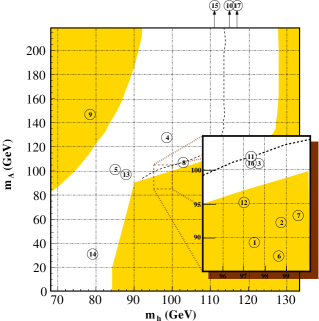
Figure 2: Schematic Distribution of the 17 cases in Table 2. The example points in Table 2 are plotted in the $(m_{h},m_{A})$ plane. Three points (Nos. 10, 15 and 17) involve pseudoscalar masses outside of the region shown. We have overlaid the “theoretically disallowed” region (light shading) and 95% exclusion contour from Figure 1 for the special case of the CP-conserving $m_{h}^{0}$-max scenario LHWG01 . These contours are shown for reference purposes only: the bounds derived for the $m_{h}^{0}$-max scenario need not apply to the 17 specific points we investigate.

III Implications for soft supersymmetry breaking

It would be very nice if one or more of the cases described in Section II pointed clearly to a simple high scale model which we could then study and perhaps motivate. Unfortunately, this does not seem to occur. The first obstacle is the fact that the Higgs sector values given in Tables 1 and 2 above do not completely specify the MSSM soft Lagrangian at the electroweak scale. Thus, translating these values to a high energy boundary condition scale $\Lambda_{\mathsc{uv}}$ through renormalization group (RG) evolution will involve some arbitrariness – for example, in choosing the low-energy values of slepton and second-generation squark masses.

In some instances, such as entry No. 8 described above, the necessary low scale values could be obtained from a unified mSUGRA model at the high scale. In order to determine how many of the low-energy scenarios of Table 1 could be similarly obtained, we performed a scan over the five parameters of the minimal supergravity model at the scale $\Lambda_{\mathsc{uv}}=\Lambda_{\mathsc{gut}}=1.9\times 10^{16}$ – unified scalar mass $m_{0}$, unified gaugino mass $m_{1/2}$, unified trilinear coupling $A_{0}$, $\tan\beta$ and the sign of the $\mu$-parameter. These parameters were evolved to the electroweak scale $\Lambda_{\mathsc{ew}}=m_{Z}$ using the code SuSpect with fermion masses and gauge coupling set to their default values SUSPECT , and the resulting Higgs sector compared with the 17 cases in Table 1. Only four of these possibilities were found to be obtainable from such a unified model at the high-energy scale, and these models are marked by a “Y” in the appropriate column of Table 1.

The fact that so few entries can be obtained from mSUGRA can be understood as follows. In general the value of the pseudoscalar mass $m_{A}$ and the coupling of the lightest CP-even Higgs to the Z-boson are related: small values of $m_{A}$ in unified models tends to require very large $\tan\beta$ which also tends to imply $C_{h}\simeq 0$. For cases in the table where $\tan\beta$ is restricted to be significantly below $\tan\beta=50$ but yet $C_{h}^{2}\neq 0$ we find no entries obtainable from mSUGRA. In addition, cases where the $\mu$ term must be large yet the pseudoscalar mass is small are not common in mSUGRA. This leaves only entries Nos. 8, 10, 16 and 17 in Table 1. For these models the values of the relevant parameters in the soft Lagrangian (and the value of the $\mu$-parameter) are given in Table 3 at the input scale $\Lambda_{\mathsc{gut}}$ and at the electroweak scale in Table 4 below.

Table 3: Soft term values at the GUT scale for models which can be obtained from the minimal supergravity paradigm. All masses are given in $~{}\mathrm{GeV}$.

	Unified Models
Entry	8	10	16	17
$M_{1}$	450	300	560	350
$M_{2}$	450	300	560	350
$M_{3}$	450	300	560	350
$A_{t}$	0	-750	0	-1300
$A_{b}$	0	-750	0	-1300
$A_{\tau}$	0	-750	0	-1300
$m_{Q_{3}}^{2}$	$(450)^{2}$	$(500)^{2}$	$(300)^{2}$	$(500)^{2}$
$m_{U_{3}}^{2}$	$(450)^{2}$	$(500)^{2}$	$(300)^{2}$	$(500)^{2}$
$m_{D_{3}}^{2}$	$(450)^{2}$	$(500)^{2}$	$(300)^{2}$	$(500)^{2}$
$m_{L_{3}}^{2}$	$(450)^{2}$	$(500)^{2}$	$(300)^{2}$	$(500)^{2}$
$m_{E_{3}}^{2}$	$(450)^{2}$	$(500)^{2}$	$(300)^{2}$	$(500)^{2}$
$m_{Q_{1,2}}^{2}$	$(450)^{2}$	$(500)^{2}$	$(300)^{2}$	$(500)^{2}$
$m_{U_{1,2}}^{2}$	$(450)^{2}$	$(500)^{2}$	$(300)^{2}$	$(500)^{2}$
$m_{D_{1,2}}^{2}$	$(450)^{2}$	$(500)^{2}$	$(300)^{2}$	$(500)^{2}$
$m_{L_{1,2}}^{2}$	$(450)^{2}$	$(500)^{2}$	$(300)^{2}$	$(500)^{2}$
$m_{E_{1,2}}^{2}$	$(450)^{2}$	$(500)^{2}$	$(300)^{2}$	$(500)^{2}$
$m_{H_{u}}^{2}$	$(450)^{2}$	$(500)^{2}$	$(300)^{2}$	$(500)^{2}$
$m_{H_{d}}^{2}$	$(450)^{2}$	$(500)^{2}$	$(300)^{2}$	$(500)^{2}$
$\mu$	-761	533	-962	730

Table 4: Soft term values at the electroweak (Z-mass) scale for models which can be obtained from the minimal supergravity paradigm. All masses are given in $~{}\mathrm{GeV}$.

	Unified Models
Entry	8	10	16	17
$\tan\beta$	39.5	25	39.5	25
$M_{1}$	179	125	237	146
$M_{2}$	344	233	452	273
$M_{3}$	1117	695	1449	812
$A_{t}$	-832	-795	-1079	-1078
$A_{b}$	-926	-1364	-1199	-1919
$A_{\tau}$	-43	-809	-61	-1312
$m_{Q_{3}}^{2}$	$(926)^{2}$	$(652)^{2}$	$(1160)^{2}$	$(674)^{2}$
$m_{U_{3}}^{2}$	$(857)^{2}$	$(491)^{2}$	$(1076)^{2}$	$(444)^{2}$
$m_{D_{3}}^{2}$	$(902)^{2}$	$(734)^{2}$	$(1118)^{2}$	$(784)^{2}$
$m_{L_{3}}^{2}$	$(519)^{2}$	$(513)^{2}$	$(491)^{2}$	$(505)^{2}$
$m_{E_{3}}^{2}$	$(413)^{2}$	$(453)^{2}$	$(329)^{2}$	$(403)^{2}$
$m_{Q_{1,2}}^{2}$	$(1129)^{2}$	$(811)^{2}$	$(1375)^{2}$	$(898)^{2}$
$m_{U_{1,2}}^{2}$	$(1094)^{2}$	$(791)^{2}$	$(1325)^{2}$	$(872)^{2}$
$m_{D_{1,2}}^{2}$	$(1089)^{2}$	$(788)^{2}$	$(1319)^{2}$	$(869)^{2}$
$m_{L_{1,2}}^{2}$	$(549)^{2}$	$(541)^{2}$	$(508)^{2}$	$(555)^{2}$
$m_{E_{1,2}}^{2}$	$(482)^{2}$	$(513)^{2}$	$(376)^{2}$	$(518)^{2}$
$m_{H_{u}}^{2}$	$-(659)^{2}$	$-(533)^{2}$	$-(841)^{2}$	$-(734)^{2}$
$m_{H_{d}}^{2}$	$-(569)^{2}$	$(375)^{2}$	$-(739)^{2}$	$(211)^{2}$
$\mu$	-569	530	-722	730

For the remaining cases, where a unified description at the high scale is nonexistent, we are forced to make some arbitrary choices for the undetermined soft Lagrangian parameters in order to reconstruct the high-energy Lagrangian. It is common practice when working with low-energy soft parameters to choose all squark masses to be degenerate for simplicity – compare, for example, the defined values of the squark masses in the “$m_{h^{0}}$-max” scenario of (9). Of course such an outcome at the electroweak scale would require a very special initial condition at the high energy scale – a fact not often appreciated in low-energy analyses. Nevertheless, fitting the Higgs sectors in Table 2 to a low-energy soft supersymmetry-breaking Lagrangian is a far easier task when the squarks are taken to be degenerate at the electroweak scale, so we will adopt that procedure here when possible. Our choices for low energy values are given in Table 5 while the translated values at the GUT scale are displayed in Table 6.

Table 5: Soft term values at the electroweak (Z-mass) scale for models which can not be obtained from the minimal supergravity paradigm. All masses are given in $~{}\mathrm{GeV}$.

	Non-universal Models
Entry	1	2	3	4	5	6	7	9	11	12	13	14	15
$\tan\beta$	6	8	10	11	32	7	13	12	14	7	19	2.5	2.1
$M_{1}$	100	100	120	300	300	100	100	300	120	100	300	200	55
$M_{2}$	200	200	240	300	300	200	200	300	240	200	300	200	250
$M_{3}$	600	600	700	1000	-1000	600	600	1000	700	600	1000	1000	700
$A_{t}$	370	430	440	500	1750	500	550	600	600	600	1750	1000	4000
$A_{b}$	400	430	440	-500	1000	400	500	500	600	500	1000	10000	4000
$A_{\tau}$	0	0	0	0	0	0	0	0	0	0	0	0	0
$m_{Q_{3}}^{2}$	$(500)^{2}$	$(500)^{2}$	$(500)^{2}$	$(500)^{2}$	$(1000)^{2}$	$(500)^{2}$	$(500)^{2}$	$(500)^{2}$	$(800)^{2}$	$(600)^{2}$	$(800)^{2}$	$(500)^{2}$	$(2000)^{2}$
$m_{U_{3}}^{2}$	$(500)^{2}$	$(500)^{2}$	$(500)^{2}$	$(400)^{2}$	$(1380)^{2}$	$(500)^{2}$	$(500)^{2}$	$(400)^{2}$	$(800)^{2}$	$(600)^{2}$	$(1200)^{2}$	$(500)^{2}$	$(2000)^{2}$
$m_{D_{3}}^{2}$	$(500)^{2}$	$(500)^{2}$	$(500)^{2}$	$(500)^{2}$	$(1000)^{2}$	$(500)^{2}$	$(500)^{2}$	$(500)^{2}$	$(800)^{2}$	$(600)^{2}$	$(800)^{2}$	$(500)^{2}$	$(2000)^{2}$
$m_{L_{3}}^{2}$	$(500)^{2}$	$(500)^{2}$	$(500)^{2}$	$(500)^{2}$	$(1000)^{2}$	$(500)^{2}$	$(500)^{2}$	$(500)^{2}$	$(800)^{2}$	$(600)^{2}$	$(800)^{2}$	$(500)^{2}$	$(2000)^{2}$
$m_{E_{3}}^{2}$	$(500)^{2}$	$(500)^{2}$	$(500)^{2}$	$(500)^{2}$	$(1000)^{2}$	$(500)^{2}$	$(500)^{2}$	$(500)^{2}$	$(800)^{2}$	$(600)^{2}$	$(800)^{2}$	$(500)^{2}$	$(2000)^{2}$
$m_{Q_{1,2}}^{2}$	$(500)^{2}$	$(500)^{2}$	$(500)^{2}$	$(500)^{2}$	$(1000)^{2}$	$(500)^{2}$	$(500)^{2}$	$(500)^{2}$	$(800)^{2}$	$(600)^{2}$	$(800)^{2}$	$(500)^{2}$	$(2000)^{2}$
$m_{U_{1,2}}^{2}$	$(500)^{2}$	$(500)^{2}$	$(500)^{2}$	$(500)^{2}$	$(1000)^{2}$	$(500)^{2}$	$(500)^{2}$	$(500)^{2}$	$(800)^{2}$	$(600)^{2}$	$(800)^{2}$	$(500)^{2}$	$(2000)^{2}$
$m_{D_{1,2}}^{2}$	$(500)^{2}$	$(500)^{2}$	$(500)^{2}$	$(500)^{2}$	$(1000)^{2}$	$(500)^{2}$	$(500)^{2}$	$(500)^{2}$	$(800)^{2}$	$(600)^{2}$	$(800)^{2}$	$(500)^{2}$	$(2000)^{2}$
$m_{L_{1,2}}^{2}$	$(500)^{2}$	$(500)^{2}$	$(500)^{2}$	$(500)^{2}$	$(1000)^{2}$	$(500)^{2}$	$(500)^{2}$	$(500)^{2}$	$(800)^{2}$	$(600)^{2}$	$(800)^{2}$	$(500)^{2}$	$(2000)^{2}$
$m_{E_{1,2}}^{2}$	$(500)^{2}$	$(500)^{2}$	$(500)^{2}$	$(500)^{2}$	$(1000)^{2}$	$(500)^{2}$	$(500)^{2}$	$(500)^{2}$	$(800)^{2}$	$(600)^{2}$	$(800)^{2}$	$(500)^{2}$	$(2000)^{2}$
$m_{H_{u}}^{2}$	$-(1689)^{2}$	$-(1491)^{2}$	$-(501)^{2}$	$-(1982)^{2}$	$-(1990)^{2}$	$-(1590)^{2}$	$-(1492)^{2}$	$-(1685)^{2}$	$-(491)^{2}$	$-(1690)^{2}$	$-(1962)^{2}$	$-(1952)^{2}$	$(392)^{2}$
$m_{H_{d}}^{2}$	$-(1679)^{2}$	$-(1480)^{2}$	$-(493)^{2}$	$-(1947)^{2}$	$-(1612)^{2}$	$-(1579)^{2}$	$-(1473)^{2}$	$-(1227)^{2}$	$-(510)^{2}$	$-(1682)^{2}$	$-(1991)^{2}$	$-(1774)^{2}$	$(403)^{2}$
$\mu$	-1700	-1500	-500	-2000	2000	-1600	-1500	-1700	500	-1700	-2000	2000	200

Table 6: Soft term values at the GUT scale for models which can not be obtained from the minimal supergravity paradigm. All masses are given in $~{}\mathrm{GeV}$.

	Non-universal Models
Entry	1	2	3	4	5	6	7	9	11	12	13	14	15
$M_{1}$	242	242	291	726	726	242	242	726	291	242	726	484	133
$M_{2}$	243	243	292	365	365	243	243	365	292	243	365	243	304
$M_{3}$	210	210	245	349	-349	210	210	349	245	210	349	349	245
$A_{t}$	3156	3292	3595	4654	4157	3573	3662	5004	4135	3931	9028	9476	33453
$A_{b}$	1564	1612	1798	1345	798	1614	1746	2418	2049	1758	3509	12514	9728
$A_{\tau}$	171	174	212	314	402	173	186	330	226	173	388	215	186
$m_{Q_{3}}^{2}$	$-(593)^{2}$	$(196)^{2}$	$(935)^{2}$	$-(788)^{2}$	$(1322)^{2}$	$(314)^{2}$	$(558)^{2}$	$(399)^{2}$	$(1422)^{2}$	$(666)^{2}$	$(2589)^{2}$	$(2614)^{2}$	$(12962)^{2}$
$m_{U_{3}}^{2}$	$-(781)^{2}$	$(414)^{2}$	$(1396)^{2}$	$-(821)^{2}$	$(2176)^{2}$	$(540)^{2}$	$(851)^{2}$	$(1003)^{2}$	$(1956)^{2}$	$(933)^{2}$	$(3822)^{2}$	$(3777)^{2}$	$(18234)^{2}$
$m_{D_{3}}^{2}$	$-(196)^{2}$	$-(197)^{2}$	$-(355)^{2}$	$-(757)^{2}$	$(160)^{2}$	$-(197)^{2}$	$-(213)^{2}$	$-(768)^{2}$	$(540)^{2}$	$(268)^{2}$	$-(409)^{2}$	$-(710)^{2}$	$(1908)^{2}$
$m_{L_{3}}^{2}$	$(470)^{2}$	$(470)^{2}$	$(454)^{2}$	$(403)^{2}$	$(1058)^{2}$	$(470)^{2}$	$(472)^{2}$	$(490)^{2}$	$(771)^{2}$	$(575)^{2}$	$(816)^{2}$	$(505)^{2}$	$(1989)^{2}$
$m_{E_{3}}^{2}$	$(487)^{2}$	$(487)^{2}$	$(486)^{2}$	$(419)^{2}$	$(715)^{2}$	$(486)^{2}$	$(484)^{2}$	$(146)^{2}$	$(794)^{2}$	$(589)^{2}$	$(582)^{2}$	$(359)^{2}$	$(1999)^{2}$
$m_{Q_{1,2}}^{2}$	$-(246)^{2}$	$-(246)^{2}$	$-(417)^{2}$	$-(772)^{2}$	$(291)^{2}$	$-(246)^{2}$	$-(247)^{2}$	$-(789)^{2}$	$(465)^{2}$	$(223)^{2}$	$-(494)^{2}$	$-(758)^{2}$	$(1890)^{2}$
$m_{U_{1,2}}^{2}$	$-(179)^{2}$	$-(179)^{2}$	$-(371)^{2}$	$-(755)^{2}$	$(676)^{2}$	$-(179)^{2}$	$-(174)^{2}$	$-(683)^{2}$	$(500)^{2}$	$(279)^{2}$	$-(167)^{2}$	$-(699)^{2}$	$(1902)^{2}$
$m_{D_{1,2}}^{2}$	$-(182)^{2}$	$-(183)^{2}$	$-(366)^{2}$	$-(733)^{2}$	$(273)^{2}$	$-(183)^{2}$	$-(185)^{2}$	$-(767)^{2}$	$(507)^{2}$	$(277)^{2}$	$-(472)^{2}$	$-(750)^{2}$	$(1902)^{2}$
$m_{L_{1,2}}^{2}$	$(470)^{2}$	$(470)^{2}$	$(454)^{2}$	$(404)^{2}$	$(1058)^{2}$	$(470)^{2}$	$(472)^{2}$	$(490)^{2}$	$(771)^{2}$	$(575)^{2}$	$(816)^{2}$	$(505)^{2}$	$(1989)^{2}$
$m_{E_{1,2}}^{2}$	$(487)^{2}$	$(487)^{2}$	$(486)^{2}$	$(419)^{2}$	$(715)^{2}$	$(487)^{2}$	$(484)^{2}$	$(147)^{2}$	$(794)^{2}$	$(589)^{2}$	$(582)^{2}$	$(359)^{2}$	$(1999)^{2}$
$m_{H_{u}}^{2}$	$-(1937)^{2}$	$-(1398)^{2}$	$(1684)^{2}$	$-(2008)^{2}$	$(902)^{2}$	$-(1441)^{2}$	$-(1062)^{2}$	$-(1809)^{2}$	$(2254)^{2}$	$-(1304)^{2}$	$(4073)^{2}$	$(4271)^{2}$	$(22213)^{2}$
$m_{H_{d}}^{2}$	$-(1690)^{2}$	$-(1493)^{2}$	$-(525)^{2}$	$-(1983)^{2}$	$-(1597)^{2}$	$-(1591)^{2}$	$-(1488)^{2}$	$-(1231)^{2}$	$-(503)^{2}$	$-(1693)^{2}$	$-(1934)^{2}$	$-(1747)^{2}$	$(390)^{2}$
$\mu$	-1687	-1479	-493	-1971	2090	-1581	-1480	-1676	494	-1680	-1995	2197	237

Naturally, entries such as Nos. 8 and 16 which can be identified with a point in the mSUGRA parameter space have a simple appearance at the high scale. By contrast, those models which have no mapping to a unified-mass model show no discernible pattern in the soft Lagrangian. While some small degree of improvement may be possible by varying those parameters left unspecified at the low scale by the Higgs sector, we have found no instances where the patterns of severe hierarchies and negative scalar mass-squareds can be alleviated. Note that these non-universal cases are particularly perverse in that both charge and color symmetries are radiatively restored in these models as the parameters are evolved towards the electroweak scale.

Even allowing for the possibility that some of the high-scale values in Table 6 which appear similar can, in fact, be made to unify with the appropriate adjustment of low scale values, we are still confronted with a large number of unrelated parameters in the soft Lagrangian. Most models of supersymmetry breaking (such as mSUGRA) are studied for their simplicity; they tend to involve very few free parameters. The traditional models of minimal gravity, minimal gauge and minimal anomaly mediation, as studied in the Snowmass Points and Slopes Snowmass ; DeHeSuWe03 have too few parameters to possibly describe these nonuniversal cases even when all three are combined in arbitrary amounts. Nor do string-based models generally provide sufficient flexibility, whether they be heterotic based bench or intersecting brane constructions such as Type IIB orientifold models IbMuRi99 . While having sufficient free parameters in the model is, strictly speaking, neither necessary nor sufficient to potentially generate one of the entries in Table 1, we feel it is a good indication of the theoretical challenge faced by models that cannot come from mSUGRA or other simple benchmark models. This is particularly true when the number of free parameters within, say, the scalar sector and the number of hierarchies in the soft Lagrangian are considered.

Table 7: Measures of fine tuning with respect to high scale parameters in Tables 3 and 6. The two entries are the sensitivities of the Z-mass and pseudoscalar mass to small changes in the input Lagrangian parameters. For example, the entries for model 1 imply that a 1% shift in high scale parameters leads to a 956% shift in the value of $m_{A}^{2}$.

Entry	$\delta_{Z}$	$\delta_{A}$	Entry	$\delta_{Z}$	$\delta_{A}$
1	1007	956	10	83.4	1.4
2	733	731	11	451	186
3	363	135	12	956	931
4	1250	632	13	2258	837
5	1117	6.3	14	3065	6.8
6	848	829	15	45573	367
7	700	718	16	196	138
8	119	94.2	17	158	1.8
9	930	4.7

That many of the entries in Table 1 imply high scale soft supersymmetry breaking patterns with such unattractive features (and no discernible theoretical structure) can be considered one element of the fine-tuning in such cases. It is not an automatic corollary, however, that the models that admit a unified explanation are necessarily less fine-tuned. In Table 7 we also provide two additional quantitative measures of the fine-tuning in these 17 cases. The numbers $\delta_{Z}$ and $\delta_{A}$ are the sensitivities of $m_{Z}$ and $m_{A}$, respectively, to small changes in the values of the independent high-scale values $a_{i}$; i.e. $\delta=\sqrt{\sum(\delta_{i})^{2}}$ where $\delta_{i}=|(a_{i}/m)\Delta m/\Delta a_{i}|$ BaGi88 .

In order to treat unified and non-unified models equally we have used the average scalar mass squared, gaugino mass and trilinear coupling as free variables in computing these sensitivities, as well as the value of the bilinear B-term (in lieu of $\tan\beta$) and the $\mu$-parameter at the GUT scale for a total of five $a_{i}$ for each model. For example, to calculate the $\delta_{m_{1/2}}$ for the nonuniversal models each gaugino mass was varied simultaneously by a certain percentage (in this case 1%). The RGEs were then solved with these three new gaugino mass input parameters and the new Z-boson mass computed at the electroweak scale. From this $\delta(m_{Z})/m_{Z}$ can be determined. The value of $\delta(m_{1/2})/m_{1/2}$ is then given by the average of the three individual perturbations divided by the average of the three original values of the gaugino masses.

As far as we can see, all models with $m_{A}\sim m_{h}$, or equivalently $C_{H}\sim 1$ are significantly fine-tuned. This is not clear from the low-scale parameters, but seems to emerge when one examines the high-scale models that give rise to small $m_{A}$. Models which require specifying multiple soft parameters quite precisely also imply additional tuning costs relative to the mSUGRA models. This should be seen as evidence of the difficulty in finding areas of the low-energy parameter space capable of producing many of the entries in Table 1. While the fine-tuning “price” of the LEP results for the MSSM has been often discussed ChElOlPo99 , it is apparent from Table 7 that the least fine-tuned result continues to be the case with $m_{h}\simeq 115~{}\mathrm{GeV}$.

IV Focus on Maximal Mixing

It may not seem surprising that the least-tuned interpretation of the LEP Higgs search is that the lightest Higgs eigenstate is Standard Model-like and very near the current limit of $m_{h}\geq 114~{}\mathrm{GeV}$, as this is the hypothesis that is so often taken when studying the constraints on the MSSM parameter space in the literature. It is perhaps more surprising that the cases with $m_{A}\sim m_{h}\sim m_{Z}$ are so much more sensitive to initial conditions, given that the magnitude of tuning in a given model is commonly associated with the importance of radiative corrections to Higgs mass eigenvalues. Yet radiative corrections are crucial in all 17 of the possible MSSM configurations – a fact that should give us pause in its own right.

Even the most “favored” possibility of $m_{h}\simeq 115~{}\mathrm{GeV}$ tends to require some superpartner masses heavier that one might naively expect, in order to obtain the $(75~{}\mathrm{GeV})^{2}$ radiative correction. In the standard mSUGRA-based studies ElHeOlWe03 ; ElNaOl02 one typically needs here either squarks or gluinos in excess of $1~{}\mathrm{TeV}$ in mass at the low energy scale, with the latter being a much more serious problem for fine-tuning than the former KaKi99 ; KaLyNeWa02 . Most of these studies assume vanishing trilinear A-terms, however. The degree of tuning can be reduced substantially if the so-called “maximal mixing” scenario can be engineered CaHeWaWe99 . In this case, the need for large superpartner masses is mitigated by maximizing the loop correction to the lightest Higgs boson mass from the $m^{2}_{\rm LR}$ entry of the stop mass matrix. In models whose scalar sector is well approximated by an overall universal scalar mass $m_{0}$, this tends to occur when $A_{t}\simeq-2m_{0}$ at the GUT scale KaKiWa01 . In models with small departures from universality this relation remains approximately correct.

To get a sense of how much the fine-tuning in the MSSM Higgs sector can be reduced when maximal mixing is achieved, consider the sole constraint on the MSSM parameter space involving a known, measured quantity

$$\frac{m_{Z}^{2}}{2}=-\mu^{2}(\mathsc{ew})+\frac{m_{H_{D}}^{2}(\mathsc{ew})-\tan^{2}\beta m_{H_{U}}^{2}(\mathsc{ew})}{\tan^{2}\beta-1},$$ (11)

where the parameters $\mu$, $m_{H_{D}}^{2}$ and $m_{H_{U}}^{2}$ are meant to be evaluated at the electroweak scale. Through the renormalization group equations these low-scale values can be translated into the high-scale input values of the entire soft supersymmetry-breaking Lagrangian KaKi99 ; deFrMu99

$$\frac{m_{Z}^{2}}{2}=\sum_{i}C_{i}m_{i}^{2}(\mathsc{uv})+\sum_{ij}C_{ij}m_{i}(\mathsc{uv})m_{j}(\mathsc{uv}).$$ (12)

For example, the leading terms in the sum (12) for $\tan\beta=10$ are found to be KaLyNeWa02

$$m_{Z}^{2} = -1.89\mu^{2}+5.58M_{3}^{2}-0.38M_{2}^{2}-0.003M_{1}^{2}$$ (13)

$$-1.20m^{2}_{H_{U}}-0.04m^{2}_{H_{D}}+0.82m^{2}_{Q_{3}}+0.66m^{2}_{U_{3}}$$

$$+0.19A_{t}^{2}-0.65A_{t}M_{3}+0.42M_{2}M_{3}+\cdots$$

where all soft terms are understood to be evaluated at the input (GUT) scale in (13).

If we were not to specialize to the case of minimal supergravity where gaugino and scalar masses are unified to the values $m_{1/2}$ and $m_{0}$, respectively, then the above equation would simplify to

$$m_{Z}^{2}\simeq-1.9\mu^{2}+5.8m_{1/2}^{2}+0.3m^{2}_{0}+0.2A_{t}^{2}-0.8A_{t}m_{1/2}.$$ (14)

Note the sizable coefficient for the gaugino mass term, especially in comparison to the relatively small coefficient in front of the scalar mass term. The bulk of these coefficients are coming from the gluino mass and the squark masses, respectively, as can be seen from the original expression (13). The size of the coefficients in (14) would seem to suggest that the result $m_{Z}=91~{}\mathrm{GeV}$ would be a “reasonable” outcome if the typical size of a soft term was on the order of tens of GeV. But direct searches for superpartners puts the typical size of these soft terms at ${\cal O}(m_{Z})$ or higher. And, as stated above, the requirement of a sufficiently large radiative correction to the Higgs mass pushes at least some of these parameters to even larger values. This is the essence of the MSSM fine tuning problem.

The coefficients in (14) are related to the sensitivity parameters $\delta_{i}$ introduced in the previous section. However, we are more concerned with the cancellations implied by (14) required to achieve $m_{Z}=91~{}\mathrm{GeV}$ than with the sensitivity of this outcome to small changes in the masses themselves. In particular, the crux of the fine-tuning problem of the MSSM Higgs sector is that a supersymmetric parameter in the superpotential – the $\mu$-parameter – must cancel to a high degree of accuracy the large contributions to the Z-boson mass coming from the soft supersymmetry-breaking Lagrangian. We are thus led to define a different variable to measure this degree of tuning.

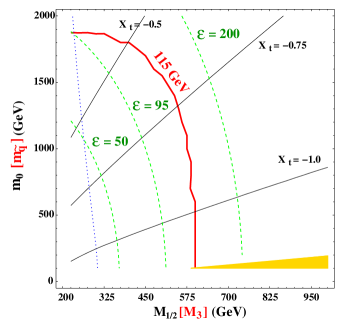
Figure 3: Economics plot for mSUGRA with $A_{0}=0$ and $\tan\beta=10$. The most efficient (least fine-tuned) point in the parameter space consistent with $m_{h}=115~{}\mathrm{GeV}$ and all observational constraints is the intersection of the Higgs mass contour (heavy solid line) and the contour of constant tuning $\epsilon=95$ (dashed line). This point intersects the contour of constant gluino mass (dotted line) for $m_{\tilde{g}}=750~{}\mathrm{GeV}$. For comparison we have included contours of constant $X_{t}$ evaluated at the electroweak scale. The shaded region in the lower right is ruled out by having a stau LSP.

For any given theory of supersymmetry breaking and transmission to the observable sector, each of the quantities on the right hand side of (12) will be determined. In general, however, the value of the $\mu$-parameter at the input scale will not be – the question of its origin typically requiring some additional model input, such as a singlet which can couple to a Higgs bilinear or the inclusion of a Giudice-Masiero term in the Kähler potential. This will be the case, for example, in the string-inspired models we will consider in the next section. We thus introduce the variable $\epsilon$ defined schematically by

$$\epsilon\equiv\frac{1}{|c_{\mu}|m_{Z}^{2}}f\left(m_{i}^{2},M_{a},A_{i}\right),$$ (15)

where $c_{\mu}$ is the coefficient of the $\mu^{2}$ term in (12) and the function $f\left(m_{i}^{2},M_{a},A_{i}\right)$ represents the terms in the summation involving the soft Lagrangian parameters. This parameter $\epsilon$ represents the tuning on $\mu^{2}$ at the high-energy scale (in units of the Z-boson mass) necessary to cancel the contribution from the soft supersymmetry-breaking sector. That is, the ratio $(\mu/m_{Z})^{2}$ would need to be tuned to roughly one part in $\epsilon$ to achieve the observed value of the Z-boson mass. This parameter is very similar to the quantity $\Phi$ introduced by Chan, Chattopadhyay and Nath to quantify cancellation in the MSSM Higgs sector ChChNa98 .

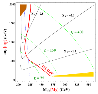
Figure 4: Economics plot for mSUGRA with $A_{0}=-2m_{0}$ and $\tan\beta=10$. The most efficient (least fine-tuned) point in the parameter space consistent with $m_{h}=115~{}\mathrm{GeV}$ and all observational constraints is the point of tangency of the Higgs mass contour (heavy solid line) and the contour of constant tuning $\epsilon=75$ (dashed line). This point intersects the contour of constant gluino mass (dotted line) for $m_{\tilde{g}}=800~{}\mathrm{GeV}$. For comparison we have included contours of constant $X_{t}$ evaluated at the electroweak scale. The shaded region in the lower right is ruled out by having a stau LSP and in the upper left by failure to break electroweak symmetry.

Armed with this variable we can safely compare different theories – and different points within the parameter space of a single theory – to determine the degree of cancellation required to achieve the correct Z-boson mass. For example, in Figure 3 we investigate the tuning implications of a 115 GeV Higgs mass within the minimal supergravity scenario with $A_{0}=0$. The contour of constant Higgs mass has the familiar form of being concave toward the origin. We have overlaid the contours of constant $X_{t}$ (determined at the electroweak scale), defined in a manner similar to that of (9) by

$$X_{t}\equiv\frac{A_{t}-\mu\cot\beta}{\sqrt{m_{t_{1}}^{2}m_{t_{2}}^{2}}},$$ (16)

where $m_{t_{1}}^{2}$ and $m_{t_{2}}^{2}$ are the values of the lighter and heavier stop mass eigenvalues, respectively. As anticipated, the case where $A_{0}=0$ at the GUT scale does not give rise to the maximal mixing scenario $X_{t}\simeq-2$ at the electroweak scale.

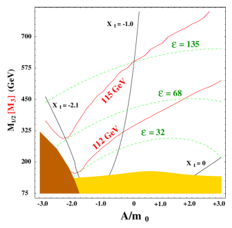
Figure 5: Gluino price plot for mSUGRA with $m_{0}=500~{}\mathrm{GeV}$. The necessary gaugino mass $m_{1/2}$ required to achieve $m_{h}=112~{}\mathrm{GeV}$ and $m_{h}=115~{}\mathrm{GeV}$ is indicated as a function of the GUT scale value of $A_{0}/m_{0}$ for $\tan\beta=10$. Note the dramatic reduction in this “price,” and the fine-tuning $\epsilon$, when $X_{t}=-2.1$ for $A_{0}\simeq-2m_{0}$. The shaded region along the bottom of the plot is ruled out by direct search constraints on chargino masses from LEP, while the darker shaded region in the lower left corner has inconsistent electroweak symmetry breaking.

To get a sense of the fine-tuning burden on the $\mu$-parameter in this space we have drawn representative contours of constant tuning $\epsilon$. Along the contour where $m_{h}=115~{}\mathrm{GeV}$, the least fine-tuned point is the point of intersection with the contour $\epsilon=95$ at the far left edge of the plot. This intersection occurs at a gluino mass of 750 GeV and the contour $m_{\tilde{g}}=750~{}\mathrm{GeV}$ is given by the dotted line in Figure 3. Note that the most “efficient” combination of soft terms for achieving $m_{h}=115~{}\mathrm{GeV}$ occurs for the smallest possible (unified) gaugino mass allowed by LEP bounds on chargino masses, with a large scalar mass. This is consistent with the relative coefficients in (12). These contours are strictly speaking functions of the universal scalar mass $m_{0}$ and universal gaugino mass $m_{1/2}$, but we keep in mind that the key masses are those of the (running) gluino mass $M_{3}$ and the typical (running) squark mass $m_{\tilde{q}}$ by including these in the axis labels. We call these plots “economics plots” for their similarity to optimization theory in which one seeks to produce a fixed amount of a good (in this case the Higgs mass) while minimizing the accompanying production of a negative externality (in this case fine-tuning).

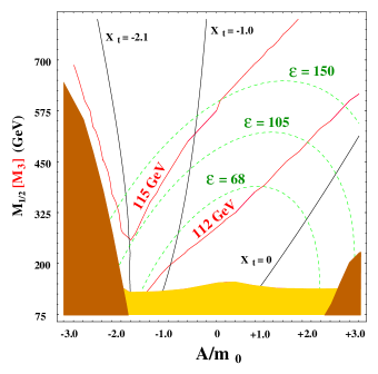
Figure 6: Gluino price plot for mSUGRA with $m_{0}=1000~{}\mathrm{GeV}$. Same plot as Figure 5 but for $m_{0}=1000~{}\mathrm{GeV}$. At these high values of the common scalar mass the value of achieving the optimal $X_{t}$ is even more profound. Again, the shaded region in the lower center of the plot is excluded by the chargino mass constraint while the darker shaded regions in the lower left and right yield inconsistent electroweak symmetry breaking.

As the value of the unified trilinear coupling $A_{0}$ is varied, the location of this optimal point will move in the $(m_{0},m_{1/2})$ plane, sweeping out a locus of optimal points. For example in Figure 4 we display the situation for $A_{0}=-2m_{0}$ at the GUT scale, again for $\tan\beta=10$. Note that the optimal point has now moved to an interior solution with moderate gaugino and scalar masses since the contour of constant Higgs mass has developed a convex form. The optimal point now occurs for $\epsilon=75$ and a gluino mass of 800 GeV (represented by the dotted contour again). Here the typical size of the mixing parameter $X_{t}$ is larger than in Figure 3 with a value very near $X_{t}=-2$ at the optimal point, as expected.

The effect of the mixing parameter $X_{t}$ is more dramatically displayed in Figures 5 and 6 for a universal scalar mass of $m_{0}=500~{}\mathrm{GeV}$ and 1000 GeV, respectively. The gaugino mass is now on the vertical axis and the ratio of $A_{0}$ to $m_{0}$ at the GUT scale on the horizontal axis. This translated into a range of values for $X_{t}$ at the electroweak scale, given by the thin, solid contours in those plots. The dramatic reduction of GUT-scale gaugino masses (the gluino “price”) required to achieve a given Higgs mass value is clearly evident at $X_{t}=-2.1$, corresponding to $A_{0}\simeq-2m_{0}$. The choice of a particular sign for this relation is the result of our conventions on defining the sign of the $\mu$-parameter (conventions opposite to those of CaElMrPiWa02 ). Clearly, the fine-tuning inherent in a given model is reduced dramatically when the relation $A_{0}\simeq-2m_{0}$ can be engineered, with important implications for the accessibility of superpartner masses at current and future colliders.

V Maximal Mixing in String Scenarios

This relation $A_{0}\simeq-2m_{0}$ is therefore an alluring goal for high-energy models, though few well-motivated models seem to naturally predict this relation. In the minimal supergravity framework both trilinears and scalar masses are taken as independent variables so no such relation is predicted. In minimal gauge mediation the trilinear couplings are negligible in relation to gaugino and scalar masses GiRa99 . While a relation between these two variables is predicted in principle in anomaly mediation, they become effectively free variables once a bulk scalar value is added to the theory to compensate for the negative slepton squared masses RaSu99 ; PoRa99 . While other solutions to this problem exist, it is this early “minimal” version of the model that was studied as part of the Snowmass Points and Slopes Snowmass . Here we prefer to focus on supergravity-based scenarios of a string-theoretic origin with the hope that this added structure will in general provide some understanding of the relation between scalar masses and soft trilinear couplings at the string or GUT scale.

String-inspired models are identified by the presence of certain gauge-singlet chiral superfields, moduli, whose Planck-scale vacuum expectation values determine the couplings of the low-energy four-dimensional theory. Thus we imagine that the gauge and Yukawa couplings of the observable sector are functions of these moduli fields (which we will denote here collectively by $\varphi^{n}$). In addition, we expect the Kähler potential for observable sector matter fields $Z^{i}$ to also be a function of these moduli and we will define

$$K(Z^{i},\overline{Z}^{i}\;\varphi^{n},\overline{\varphi}^{n})=\kappa_{i}(\varphi^{n},\overline{\varphi}^{n})|Z^{i}|^{2}+{\cal O}(|Z^{i}|^{4}).$$ (17)

The relation between the tree-level trilinear coupling $(A_{0})_{ijk}$ and the tree-level scalar mass $(m_{0}^{2})_{i}$ at the boundary condition scale is then determined by the functional dependence of the various couplings on the moduli. For any supergravity model we have the fundamental relations

$$(A_{0})_{ijk} = \left\langle K_{n}F^{n}-F^{n}\partial_{n}\ln(\kappa_{i}\kappa_{j}\kappa_{k}/W_{ijk})\right\rangle$$

$$(m_{0}^{2})_{i} = m_{3/2}^{2}-\left\langle F^{n}\overline{F}^{\bar{m}}\partial_{n}\partial_{\bar{m}}\ln\kappa_{i}\right\rangle$$ (18)

where $F^{n}$ is the auxiliary field of the chiral superfield associated with the modulus $\varphi^{n}$, $m_{3/2}$ is the gravitino mass, $W_{ijk}$ is the (generally moduli dependent) Yukawa coupling between observable sector fields and $K_{n}=\partial K/\partial\varphi^{n}$. A summation over all moduli $\varphi^{n}$ which participate in communicating supersymmetry breaking via $\left\langle F^{n}\right\rangle\neq 0$ is implied in (18). For a fuller description of soft terms in a general supergravity theory, as well as the string models we will present below, the reader is referred to the Appendix.

Neglecting possible D-term contributions to the scalar potential, the value of the potential in the vacuum is given by

$$\left\langle V\right\rangle=\left\langle K_{n\bar{n}}F^{n}\overline{F}^{\bar{n}}\right\rangle-3m_{3/2}^{2},$$ (19)

where a summation over moduli is again implied and $K_{n\bar{n}}=\partial^{2}K/\partial\varphi^{n}\partial\overline{\varphi}^{\bar{n}}$. Requiring that this contribution to the cosmological vacuum energy vanish leads to a relation between the gravitino mass and the supersymmetry breaking scale governed by the various $\left\langle F^{n}\right\rangle$. For the remainder of this section we will investigate various string scenarios using the general expressions in (17) and (18) to search for cases where $A_{0}\simeq 2m_{0}$ can be obtained.

V.1 Naive dilaton domination

The simplest string-based scenario is the case of dilaton domination. For the weakly-coupled heterotic string the gauge couplings of the low-energy theory are determined by the vacuum value of a single modulus field, the dilaton $S$. This field does not participate in the Yukawa couplings or the observable sector Kähler metric (17). By dilaton domination we refer to a situation in which this is the only modulus whose auxiliary field gets a nonvanishing vacuum value. The tree level Kähler potential for the dilaton is simply $K(S,\overline{S})=-\ln(S+\overline{S})$ and thus the dilaton domination scenario is a natural realization of the special case

$$\frac{A_{0}^{2}}{(m_{0}^{2})_{i}}=3\left\langle\frac{K_{s}K_{\bar{s}}}{K_{s\bar{s}}}\right\rangle\to 3.$$ (20)

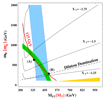
Figure 7: Economics plot for the dilaton domination scenario with $\tan\beta=10$. The subset of points in the mSUGRA plane that can be obtained from the dilaton domination scenario are given by the dashed line. An optimal scenario for a 115 GeV Higgs mass would be the point labeled (A), but the dilaton domination paradigm only allows us to be at point (B) to satisfy this constraint. The difference in tuning parameter $\epsilon$ is given by the dark shaded region, bounded on the interior by $\epsilon=84$ and on the exterior by $\epsilon=100$. The difference in gluino masses is even more profound, represented by the light shaded region bounded by $m_{\tilde{g}}=875~{}\mathrm{GeV}$ on the left and $m_{\tilde{g}}=1153~{}\mathrm{GeV}$ on the right.

This string-inspired scenario has been studied at length in the literature BrIbMu94 ; BrIbMuSc97 ; Ir98 ; AbAlIbKlQu00 . It is a special case of the minimal supergravity scenario with the following soft terms

$$M_{a} = \sqrt{3}\left(\frac{g_{a}^{2}(\mathsc{uv})}{g_{\mathsc{str}}^{2}}\right)m_{3/2}$$

$$A_{0} = -\sqrt{3}m_{3/2}$$

$$m_{0}^{2} = m_{3/2}^{2},$$ (21)

where we have chosen conventions such that gaugino masses are positive. If we take the input string scale $\Lambda_{\mathsc{str}}$ to be the same as the GUT scale, neglecting the small difference between these two scales Ka88 we arrive at the famous relation among the soft terms $m_{1/2}=-A_{0}=\sqrt{3}m_{0}$. As this model is a subclass of mSUGRA models we can study it in the same way we studied the general cases of Section IV.

For example, in Figure 7 we plot the same parameter space as Figures 3 and 4 for $\tan\beta=10$. The dilaton domination assumption requires the theory to lie on the locus of points identified by the heavy dashed line, where $X_{t}\simeq 1.3$ at the electroweak scale. In this model, with $A_{0}=-\sqrt{3}m_{0}$ the optimal point that gives rise to $m_{h}=115~{}\mathrm{GeV}$ is the point labeled by (A) with tuning $\epsilon=84$ and gluino mass $m_{\tilde{g}}=875~{}\mathrm{GeV}$ (the inside contours of the heavy and light shaded regions, respectively). The only way to achieve this Higgs mass value in the dilaton domination scenario is to be at point (B) with a slightly greater amount of fine-tuning $\epsilon=100$ but a much heavier gluino mass $m_{\tilde{g}}=1153~{}\mathrm{GeV}$ (the outside contours of the heavy and light shaded regions, respectively). While the optimal point cannot be reached, the topology of the Higgs mass contour is what we expect as we approach the maximal mixing scenario, and this represents a general improvement in the fine-tuning overall in this model.

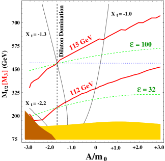
Figure 8: Gluino price plot for dilaton domination with $m_{0}=280~{}\mathrm{GeV}$. The subset of points for which $A_{0}/m_{0}=-\sqrt{3}$ as in the dilaton domination scenario are given by the vertical dashed line. At intersection of this contour with the contour for $m_{h}=115~{}\mathrm{GeV}$ we have $X_{t}\simeq 1.3$ and $\epsilon=100$. The dotted horizontal line is a gluino mass of $m_{\tilde{g}}=1150~{}\mathrm{GeV}$. For lower Higgs masses the dilaton domination scenario moves closer to the optimal point in the lower left corner where $X_{t}\simeq-2.2$. The excluded shaded regions are the same as Figure 5.

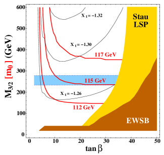
Figure 9: Parameter space for the dilaton domination scenario. Increasing $\tan\beta$ from $\tan\beta=10$ to $\tan\beta=32$ along the contour $m_{h}=115~{}\mathrm{GeV}$ allows a marginally lighter gluino. The horizontal shaded region is bounded above by the contour $m_{\tilde{g}}=1150~{}\mathrm{GeV}$ and below by the contour $m_{\tilde{g}}=975~{}\mathrm{GeV}$. Note that throughout the relevant parameter space of this model $X_{t}\simeq-1.3$ at the electroweak scale. The lighted shaded region is ruled out by the requirement that the LSP be neutral, while the darker shaded region has inconsistent electroweak symmetry breaking.

Nevertheless, the dilaton domination scenario moves further from the optimal point as the Higgs mass constraint increases. In Figure 8 we present the analogous plot to Figure 5, with the restricted space of the dilaton domination paradigm indicated by the dashed vertical line. At lower Higgs mass values the necessary gluino mass is smaller, resulting in less fine-tuning and the optimal value of $X_{t}$ needed to achieve the maximal mixing scenario approaches the value dictated by the soft-term constraints of this model. Some marginal improvement in fine tuning can, of course, be obtained by increasing the value of $\tan\beta$ beyond the value studied in Figures 7 and 8. For example, in Figure 9 we display the entire parameter space for this model, defined as it is by $\tan\beta$ and one overall mass scale, which we take to be the scalar mass. For $\tan\beta=10$ we see that $m_{h}=115~{}\mathrm{GeV}$ requires $m_{\tilde{g}}=1150~{}\mathrm{GeV}$ at the electroweak scale (the top contour of the horizontal shaded region) as before. At the maximal value of $\tan\beta$ for this Higgs mass allowed by the requirement of a neutral lightest supersymmetric particle (LSP), specifically $\tan\beta=32$, the gluino mass can be lowered to 975 GeV (the bottom contour of the horizontal shaded region).

So we conclude that the generic point in the parameter space of this string-motivated scenario involves less cancellation in the relation (11) for a given Higgs mass than a generic point in the full mSUGRA parameter space. But the tuning is still sizable and the model requires a relatively large gluino mass. This latter problem can be remedied by invoking a different modulus field from the string theory to perform the role of transmitting the supersymmetry breaking from a hidden sector to the observable sector.

V.2 Nonuniversal modular weights

While the kinetic functions of observable sector matter fields are typically not functions of the dilaton – at least in the case of the weakly coupled heterotic string – they typically are functions of the so-called Kähler moduli $T^{I}$ whose vacuum values determine the size of the compact space. In what follows we will assume, for the sake of simplicity, that observable sector quantities depend only on a single overall modulus $T$. At the leading order the functional dependence of the Kähler metric for the fields $Z^{i}$ on this modulus is given by

$$\kappa_{i}=(T+\overline{T})^{n_{i}}$$ (22)

where $n_{i}$ is referred to as the modular weight of the field $Z^{i}$. These weights depend on the sector of the string Hilbert space from which the field arises and are typically negative integers $n_{i}=-1,\;-2,$ etc.

In the limit where only this overall Kähler modulus breaks supersymmetry (i.e. only $\left\langle F^{T}\right\rangle\neq 0$) the scalar masses take the tree-level form

$$(m_{0}^{2})_{i}=(1+n_{i})m_{3/2}^{2}$$ (23)

where we have employed the second line of (18) and again assumed vanishing vacuum energy at the minimum. Note that in this Kähler modulus-dominated limit, when the modular weight of a field takes the value $n_{i}=-1$, then the scalar mass vanishes at this order. For values $n_{i}=-2,\;-3$, etc. the scalar masses are imaginary at the input scale. When the scalar mass vanishes at the tree level we must compute the one-loop correction to the tree-level value in the supergravity theory. This calculation has been performed GaNe00b ; BiGaNe01 and the leading correction in this limit is given by $(m_{1}^{2})_{i}=(m_{0}^{2})_{i}+\delta m_{i}^{2}$ with $\delta m_{i}^{2}=\gamma_{i}m_{3/2}^{2}$.

In order to determine the trilinear A-terms in this framework we must know the dependence of the Yukawa couplings of the observable sector on the Kähler moduli. These can be obtained from symmetry arguments inherited from the underlying string theory and have been verified by direct computation DiFrMaSh87 ; FoIbLuQu90 . They involve the Dedekind function

$$\eta(T)=e^{-\pi T/12}\prod_{n=1}^{\infty}(1-e^{-2\pi nT})$$ (24)

in a particular combination determined by the modular weights of the fields involved in the coupling

$$W_{ijk}=\lambda_{ijk}\left[\eta(T)\right]^{-2(3+n_{i}+n_{j}+n_{k})}.$$ (25)

The Kähler potential for the (overall) modulus $T$ is given by $K(T,\overline{T})=-3\ln(T+\overline{T})$ so that the two terms in the first line of (18) combine to form

$$(A_{0})_{ijk}=(3+n_{i}+n_{j}+n_{k})\left\langle G_{2}\left(t,\bar{t}\right)\right\rangle m_{3/2}$$ (26)

where $G_{2}\left(t,\bar{t}\right)$ is the Eisenstein function

$$G_{2}\left(t,\bar{t}\right)\equiv\left(2\frac{1}{\eta(t)}\frac{d\eta(t)}{dt}+\frac{1}{t+\bar{t}}\right)$$ (27)

and $t$ is the lowest component of the chiral superfield $T$.

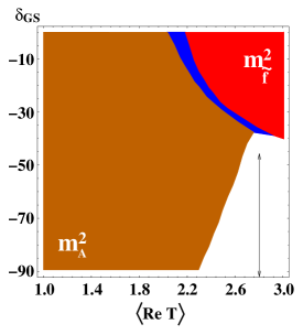
Figure 10: Parameter space for the moduli domination scenario with $n_{H_{u}}=n_{H_{u}}=-2$ and $\tan\beta=10$. The large shaded area marked $m_{A}^{2}$ has an imaginary pseudoscalar mass and is ruled out. The shaded area in the upper right marked $m_{\tilde{f}}^{2}$ has an imaginary running mass for one or more third-generation scalar fermions. The shaded area in between these two regions is ruled out as at least one physical mass eigenstate for the scalar fermions is imaginary due to mixing effects. The region of the parameter space examined in Figure 11 is marked by the vertical arrow at $\left\langle{\rm Re}\;T\right\rangle=2.8$.

The last quantity we need is the soft gaugino mass for the three observable sector gauge groups. As mentioned above, at the leading order the gauge kinetic function for all gauge groups in the weakly coupled heterotic string is simply the dilaton $S$. Therefore, in the Kähler modulus-dominated regime the gaugino masses vanish at the leading order at the string scale. At the one-loop level the corrections to the gaugino masses involve the Kähler moduli and take the form GaNeWu99

$$M_{a}=\frac{g_{a}^{2}}{16\pi^{2}}m_{3/2}\left[b_{a}+k_{a}\left\langle(t+\bar{t})G_{2}\left(t,\bar{t}\right)\right\rangle\right]$$ (28)

where

$$k_{a}=\delta_{\mathsc{gs}}+b_{a}-2\sum_{i}C_{a}^{i}(1+n_{i}),$$ (29)

$b_{a}$ is the beta-function coefficient for the group $\mathcal{G}_{a}$ with $b_{a}=3C_{a}-\sum_{i}C_{a}^{i}$, and $\delta_{\mathsc{gs}}$ is the coefficient of the Green-Schwarz counterterm introduced to restore modular invariance to the theory DiKaLo91 ; DeFeKoZw92 ; GaTa92 . For the purposes of this section it is only necessary to know that this parameter is calculable from the underlying orbifold compactification and is a negative integer in the range $\delta_{\mathsc{gs}}\in[0,-90]$. Details on the origin of these expressions can be found in the Appendix.

The appearance of new free parameters, such as $\delta_{\mathsc{gs}}$ and the various modular weights $n_{i}$, as well as the modular functions $G_{2}\left(t,\bar{t}\right)$ and $(t+\bar{t})G_{2}\left(t,\bar{t}\right)$, would seem to indicate a greater degree of freedom in relating the scalar masses to the trilinear scalar couplings. Often in the literature this “moduli-dominated” regime is studied in the limit where $n_{i}=-1$ for all fields. This would be the case, for example, if all observable sector matter were untwisted states of the underlying string theory. This limit was referred to as the “O-II” model in BrIbMu94 . In fact, explicit surveys of semi-realistic orbifold models Gi02 indicate that at least some subset of MSSM fields must be given by twisted-sector states for which $n_{i}=-2,\;-3,\;\dots$. This case was referred to as an “O-I” model in BrIbMu94 .

But when $|n_{i}|>1$ in this modulus-dominated limit the corresponding scalar mass squared is negative. We might not consider this a troubling feature of the model if it is one or more of the Higgs scalar masses that are imaginary at the string scale. For example, if we consider the case $n_{H_{u}}=-2$; $n_{Q_{3}}=n_{U_{3}}=-1$, then the field $H_{u}$ will have a negative squared mass of ${\cal O}(m_{3/2}^{2})$, the top quark trilinear coupling $A_{t}$ will also be negative and of ${\cal O}(m_{3/2})$ while the gaugino masses and squark masses will be smaller by roughly an order of magnitude. Can such a set of boundary conditions give rise to a reasonable low-energy spectrum of soft terms? We surveyed the three cases $(n_{H_{u}},n_{H_{d}})=(-2,-1),\;(-1,-2)$, and $(-2,-2)$ but found only the last case had any viable parameter space. This is hardly surprising, since the first two cases give rise to large hypercharge D-term contributions to the RG evolution of scalar quarks and leptons, causing at least some set of these fields to develop negative squared masses at the electroweak scale and thereby presumably triggering the spontaneous breaking of color and electric charge. The viable parameter space in the $(\delta_{\mathsc{gs}},\left\langle{\rm Re}\;T\right\rangle)$ plane for the case $(n_{H_{u}},n_{H_{d}})=(-2,-2)$ is given in Figure 10. The large shaded region labeled $m_{A}^{2}$ gives rises to an imaginary pseudoscalar mass at the electroweak scale. In the upper right shaded region labeled $m_{\tilde{f}}^{2}$ one of the third-generation running scalar masses is imaginary at the low-energy scale. A representative slice of the remaining allowed parameter space, represented by the vertical double-arrow in Figure 10 is plotted in Figure 11.

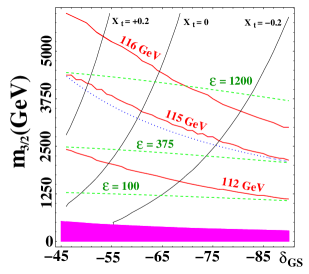
Figure 11: Economics plot for the moduli domination scenario with $n_{H_{u}}=n_{H_{u}}=-2$. Despite the relatively large trilinear coupling $A_{t}$ the low-energy soft Lagrangian for this model is essentially a minimal-mixing scenario. The dotted line represents the contour $m_{\tilde{g}}=2400~{}\mathrm{GeV}$. Depending on the value of the Green-Schwarz coefficient, the cancellation coefficient lies in the range $375\leq\epsilon 1200$ for $m_{h}=115~{}\mathrm{GeV}$. The shaded region at the bottom of the plot is ruled out by direct search limits for gluinos and/or charginos.

Despite the fact that the top-quark trilinear coupling (and indeed, all third-generation trilinear couplings) are large relative to the typical squark and slepton mass, this model flows in the infrared to a minimal-mixing scenario at low energies. The typical size of $X_{t}$ in Figure 11 is $-0.3\leq X_{t}\leq 0.3$. The contours of constant Higgs mass nearly track those of constant gluino mass: for example, the contour $m_{h}=115~{}\mathrm{GeV}$ lies very near the contour $m_{\tilde{g}}=2400~{}\mathrm{GeV}$. As the value of $\delta_{\mathsc{gs}}$ increases, the absolute value of the gluino mass increases as well, allowing the same value of $m_{h}$ for a lower overall scale of soft terms – and hence a smaller amount of fine-tuning at the electroweak scale. Yet given the string/GUT scale relation $m_{H_{u}}^{2}\sim-m_{3/2}^{2}$, the large mass scale necessary to ensure sufficiently large gaugino masses puts enormous pressure on the high-scale value of the $\mu$ parameter to compensate the large positive contribution to $m_{Z}^{2}$ in (13). Far from improving the situation of the generic mSUGRA model, this limit in the string moduli space is as fine-tuned as the worst of the models in Table 7.

V.3 A model based on D-branes at intersections

The previous two string-based scenarios derived from the weakly coupled heterotic string. It might be thought that the inability to easily obtain the maximal mixing scenario in the Higgs sector is the result of the restrictive nature of these models. The moduli sector of open string models is far richer than the heterotic string, with more fields appearing in each of the three functions relevant to the low energy supergravity Lagrangian: the observable sector gauge kinetic functions, the Kähler metric for the MSSM fields and the Yukawa couplings of the observable sector superpotential.

For example, in orientifold compactifications of Type I/Type IIB string theory – close relatives to the orbifold compactification of the heterotic string studied above – Kähler moduli now appear at the leading order in gauge kinetic functions, while the dilaton field can appear in the Kähler potential for the MSSM fields AnBaFaPaTa97 ; AlFoIbVi99 . The study of four-dimensional effective supergravity Lagrangians representing these theories is a subject of ongoing research. Many of the early studies, such as IbMuRi99 , were ultimately based on the well-known results of the weakly-coupled heterotic string with duality symmetries invoked to map those results to the open string theory in the case Type I and Type IIB models. Not surprisingly, then, these effective Lagrangians share many of the same structures and features of their heterotic counterparts. While it is now possible to study in greater detail the full richness of open string models, we prefer to restrict ourselves to a particularly simple configuration which closely resembles the models we studied above and leave a more complete survey to future work.

Let us consider a particular configuration of Type IIB theory compactified on an orientifold with intersecting $D_{5}$-branes. The world volume of these extended objects is six-dimensional and is assumed to span 4D Minkowski space plus two of the six compact dimensions. The six dimensional compact space is assumed to factorize into three compact torii, each with a radius dictated by the vacuum value of an associated Kähler modulus $T^{I}$. We then associate each of the sets of $D_{5}$ branes with a particular torus in the compact space spanned by its world volume with associated modulus $T^{I}$. As the gauge coupling on each stack of $D_{5}$ branes is determined by the vev of the associated $T^{I}$, we will assume, for the sake of simplicity, that the inverse radii of all the compact torii are the same and that all three moduli participate equally in supersymmetry breaking. Then gaugino masses will be unified at the boundary-condition scale as well: $M_{1}=M_{2}=M_{3}$.

So far this is similar to the dilaton-dominated scenario of the heterotic string theory. The novelty in this case is that the MSSM matter content is represented by open strings which can connect sets of 5-branes whose world volumes span different complex compact dimensions. Fields represented by the massless modes of these strings will be denoted by two subscripts. For example, a field $Z^{i}$ which is the massless mode of a string that stretches from a set of branes $5_{I}$ to a non-parallel set $5_{J}$ will be written $Z^{i}_{IJ}$. For these fields the Kähler potential is given by (17) where

$$\kappa_{i}^{IJ}=\frac{1}{2}(S+\overline{S})^{-1/2}(T^{K}+\overline{T}^{K})^{-1/2},$$ (30)

and the particular Kähler modulus $T^{K}$ is identified by the requirement that $I\neq J\neq K\neq I$ IbMuRi99 . The Kähler potential for the moduli fields continues to be given by the leading-order form $K=-\ln(S+\overline{S})-\sum_{I=1}^{3}\ln(T^{I}+\overline{T}^{I})$. Following IbMuRi99 we take the Yukawa couplings of the observable sector to be independent of these moduli fields at the leading order. A particularly simple model is obtained when all MSSM fields are represented by such stretched strings – a case we will call the “universally stretched” regime. When the Kähler moduli have equal vacuum values (as we assumed above) and participate equally in supersymmetry breaking, the soft terms for the model are

$$M_{a} = \left(\frac{g_{a}^{2}(\mathsc{uv})}{g_{\mathsc{str}}^{2}}\right)m_{3/2}$$

$$A_{0} = -\frac{3}{2}m_{3/2}$$

$$m_{0}^{2} = \frac{1}{2}m_{3/2}^{2}.$$ (31)

To obtain (31) we once again used the assumption that the scalar potential has vanishing vacuum value. Note that this is a special case of the general mSUGRA paradigm, but in this case $A_{0}=-3/\sqrt{2}m_{3/2}$ and thus the universally stretched regime represents a potential improvement in tuning over the dilaton dominated limit.

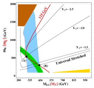
Figure 12: Economics plot for the Type IIB brane model with universally stretched strings. The subspace of the mSUGRA model with the soft terms given in (31) is denoted by the labeled dashed line. The similarity of this plot to the dilaton-dominated model of Figure 7 is the result of our insistence upon gauge coupling unification at the string scale. An optimal scenario for a 115 GeV Higgs mass would be the point labeled (A), but this brane model only allows us to be at point (B) to satisfy this constraint. The difference in tuning parameter $\epsilon$ is given by the dark shaded region, bounded on the interior by $\epsilon=70$ and on the exterior by $\epsilon=90$. The difference in gluino masses is even more profound, represented by the light shaded region bounded by $m_{\tilde{g}}=750~{}\mathrm{GeV}$ on the left and $m_{\tilde{g}}=1050~{}\mathrm{GeV}$ on the right.

Comparing the economics plot of this model in Figure 12 with that of the dilaton domination model of Figure 7 it is clear that there is an improvement in the fine-tuning, but that this improvement is small. The locus of points in the mSUGRA parameter space that are consistent with (31) are given by the labeled dashed line. The optimal point for $m_{h}=115~{}\mathrm{GeV}$ in Figure 12 is in nearly the same location in the $(m_{1/2},m_{0})$ plane as in Figure 7, with $\epsilon=70$ and $m_{\tilde{g}}=750~{}\mathrm{GeV}$. But the contours of constant tuning parameter $\epsilon$ have moved inwards towards the origin, reflecting the increased value of $X_{t}$ at the electroweak scale. As a result, the required low-scale gluino mass at the point where the dashed line and $m_{h}=115~{}\mathrm{GeV}$ contour intersect is $m_{\tilde{g}}=1050~{}\mathrm{GeV}$ with $\epsilon=90$ there.

As in the dilaton dominated case we conclude that tuning in the electroweak sector is generally mitigated in the universally stretched model relative to a generic point in the mSUGRA parameter space due to the relation between trilinear scalar couplings and scalar masses at the high scale. Yet we are still left with uncomfortably heavy gauginos (especially gluinos) and the constrained nature of the paradigm will not allow us to reach the “optimal” point for achieving $m_{h}=115~{}\mathrm{GeV}$ while simultaneously ensuring $m_{Z}=91~{}\mathrm{GeV}$.

V.4 More sophisticated models

So far we have chosen to look at three particularly simple directions in the string moduli space. We have done so in part to keep the level of technical detail low – a beginning approach we feel is justified in a first examination of the theoretical implication of the LEP Higgs search. But there is also a reason of analytical simplicity: the key variable in achieving the maximal Higgs mass with the least cancellation in (11) is the value of the stop mixing parameter $X_{t}$ at the electroweak scale. On the other hand, models of supersymmetry breaking and transmission to the observable sector descended from string theory give relations among soft terms at a very high energy scale. The two can be related in a straightforward manner (i.e. $A_{0}\simeq-2m_{0}$ at the GUT scale implies $X_{t}\simeq-2$ at the Z-mass) only in certain restrictive regimes, such as a model with a high degree of universality among soft scalar masses. Departures from the simplifying assumptions made above will necessarily lead to nonuniversalities in the scalar sector and a much fuller analysis is necessary to determine how readily $X_{t}\simeq-2$ is achieved at the low scale. We do not wish to perform that analysis here, but we do wish to comment on what types of models might allow the freedom necessary to reach the maximal mixing scenario.

In subsections B and C we imagined scenarios in which Kähler moduli dominate the supersymmetry breaking in the observable sector – moduli which appear in the tree-level Kähler metric for matter fields. When we study top-down models directly tied to the underlying string theory we imagine this functional dependence to be that of (22) with $n_{i}=-1,\;-2,\;-3$ for weakly coupled heterotic models on orbifolds or $n_{i}=0,\;-1/2,\;-1$ for Type I/IIB models on orientifolds. The restrictive nature of these choices kept us from realizing a phenomenologically optimal scenario. However, if it were possible to treat these modular weights as arbitrary – even continuous parameters – it would not be at all difficult to construct situations with the desired properties. To what extent is such a treatment justified?

As mentioned previously, the modular weights are related to what sector of the string Hilbert space each light field arises from. Just below the string scale, when the four dimensional effective Lagrangian is first defined, these weights are indeed constrained to the values mentioned above. However, in the weakly coupled heterotic string we are compelled to make sure that our effective Lagrangian respects modular invariance. This symmetry should continue to hold even after any anomalous U(1) factor is integrated out of the theory. Thus, fields which take vacuum values to cancel the anomalous U(1) FI term must be removed from the theory in modular invariant (and U(1) invariant) combinations. For example, if the field $Y$ carries anomalous U(1) charge $q_{Y}^{X}$ and acquires a vacuum value $\left\langle Y\right\rangle\neq 0$, then the appropriate combination to integrate out of the theory is GaGi02a ; GaGi02b

$$\left\langle e^{2q_{Y}^{X}V^{X}}(T+\overline{T})^{n_{Y}}|Y|^{2}\right\rangle,$$ (32)

where $V_{X}$ is the vector superfield representing the anomalous U(1) and $n_{Y}$ is the modular weight of the field $Y$.

The result of removing this combination of fields from the theory is to shift the effective modular weight of the remaining light fields, if those fields also carry an anomalous U(1) charge. The amount of this shift is given by

$$n_{i}\to(n_{i})^{\prime}=n_{i}-q_{i}^{X}\times\left(\frac{n_{Y}}{q^{X}_{Y}}\right)$$ (33)

where $q_{i}^{X}$ is the anomalous U(1) charges of the light field in question. Given the typical sizes of these charges Gi02 there is every reason to expect that the resulting modular weights, if modified at all, will take quite unorthodox and generally non-integral values. The question of whether this effect will produce the desired relation between A-terms and scalar masses – and indeed, whether it occurs at all – is a model-dependent one.

Another way to generalize the above cases is to modify the functional dependence of the Yukawa couplings and Kähler metrics of the MSSM fields on the various string moduli. For example, strongly coupled heterotic strings bring the dilaton into play even at the tree level for these quantities, while the Kähler moduli appear at the leading order in gauge kinetic functions. Even in the weakly coupled case it is possible to introduce some non-trivial dilaton dependence into A-terms and scalar masses if observable sector matter couples to the Green-Schwarz anomaly-cancellation term GaNe00a . If the GS counterterm depends on the radii of the three compact torii via the combination $(T^{I}+\overline{T}^{I}-\sum_{i}|Z_{i}^{I}|^{2})$, where $Z_{i}^{I}$ is a matter field which carries a modular weight under the modulus $T^{I}$, then even in the dilaton-dominated limit there is an effect on the soft supersymmetry breaking terms due to the kinetic mixing induced by the Green-Schwarz counterterm.

Finally, we might expand the space of possible outcomes by considering models with a richer moduli spectrum to begin with. The orbifold models that inspired the cases A and B above were based on the $Z_{3}$ orbifold, for which the complex structure of the compact space is completely fixed by the supersymmetry requirements. As such, it does not have free parameters that would be represented in the low-energy four dimensional theory as complex structure moduli. Such fields do appear, however, in the leading order supergravity effective Lagrangian describing other orbifold models of the heterotic string IbLu92 , as well as models based on open string theories. For example, in the Type IIA models the gauge kinetic functions depend on complex structure moduli, with the Kähler moduli appearing only at the loop level to cancel anomalies CrIbMa02 ; LuSt03 . This is analogous to the introduction of Kähler moduli into the formula for the gaugino masses at the loop level in the heterotic string by the presence of a Green-Schwarz counterterm (c.f. equation 28 above). The open string model studied in case C above was chosen for its extreme simplicity, as a first departure from the confines of the weakly-coupled heterotic case. But much more complicated structures are likely to appear in more realistic constructions. At the loop level in Type I/IIB models anomaly cancellation requirements introduce new twisted moduli into the gauge kinetic functions: the “blowing-up” modes which parameterize the transition from the singular manifold represented by the orientifold to the presumably more realistic smooth manifold it is meant to approximate IbRaUr99 ; AnBaDu99 . Thus in open string models we might expect greater freedom to find cases where $A_{0}\simeq-2m_{0}$ is a robust prediction. It would be of great interest to search the (generally non-universal) models based on orientifold compactification of Type I/Type II string theory for points where $m_{Z}=91~{}\mathrm{GeV}$ appears as a natural outcome of the supersymmetry breaking as the effective Lagrangians describing these models become more realistic.

Conclusion

We began this work asking the question, “Where do we stand after LEP II?” Accepted wisdom following the lack of a Higgs discovery at LEP has been that if the MSSM is the correct description of nature just above the electroweak scale then the lightest Higgs boson is at least 115 GeV in mass and very Standard Model-like in its properties. It is further generally accepted that this implies an uncomfortable level of fine-tuning in the underlying supersymmetric Lagrangian, though precisely how much and how unsettling is a somewhat subjective matter. Is this post-LEP conclusion inevitable?

To answer this we looked at the data to find all the logically distinct ways that the MSSM can be a correct description yet produce no Higgs discovery at LEP. In total we found 17 such possibilities – representing the primary purpose behind this work. The majority of these cases involve Higgs bosons with masses below the 115 GeV limit, though the parameter space for each of these models are generally not of the same size. While all cases are logically on an equal, a priori footing not all are equally “tuned.” When the issue of large cancellations between soft Lagrangian parameters and the $\mu$ parameter are included in the comparison, the conventional wisdom of the post-LEP electroweak sector is seen as the most “plausible” outcome.

Given this hypothesis – based as it is on fine-tuning as a tool – what are the LEP results telling us about high-scale theories? Can we follow our nose and light upon a preferred outcome? From the bottom-up approach it is quite easy to engineer situations where the relation $A_{0}\simeq-2m_{0}$ arises at high energy scale. The difficulty is in finding such a construction that is also motivated by an underlying theory such as string theory. Starting here with some simple top-down approaches it appears that this preferred model is not yet obvious. So if we are committed to weak scale supersymmetry as a low-energy effective Lagrangian derived ultimately from some sort of string theory, then we find ourselves at a fork in the road. Should nature really be described by the minimal supersymmetric version of the Standard Model then LEP may be suggesting a more complicated string model than the simple ones we typically study – or perhaps special points in the moduli space of these theories. On the other hand, it may simply be that the ultimate supersymmetric Standard Model is not minimal – see, for example, Ref. BaHuKiRoVe00 . This would not be surprising as we often find precisely such extended theories from top-down studies of string models.

If fine-tuning is really a worthwhile concept for the theoretical physicist, then its utility lies in directing our focus towards those theories that are most compatible with nature when data is lacking or ambiguous. In this role the LEP data can still serve a valuable purpose, despite the lack of a Higgs discovery. Assuming that an appropriately defined measure of fine-tuning is truly telling us something about nature, then studies which probe well-defined departures from the minimal model can utilize the LEP data to identify promising avenues for further research

Appendix

In this appendix we present the derivation of the soft supersymmetry breaking terms at the tree level in string-derived supergravity theories. We provide specific expressions for modular invariant supergravity theories from weakly-coupled heterotic strings, as well as expressions for models based on orientifold compactification of Type-I/Type-IIB open string theories. More details and loop corrections to these expressions for the weakly-coupled heterotic string can be found in BiGaNe01 .

Of particular importance for the question of supersymmetry breaking are the types of string moduli present in the low-energy theory and their couplings to the observable fields of the MSSM CvLoOv88 ; DiKaLo90 ; DiKaLo91 . Gaugino masses will depend on auxiliary fields related to moduli appearing in the gauge kinetic function, while scalar masses, trilinear A-terms and bilinear B-terms will depend on auxiliary fields related to those moduli that appear in the superpotential couplings and/or Kähler potential for the MSSM fields KaLo93 ; BrIbMu94 . The precise form of these soft terms can be obtained by working out the component Lagrangian for the observable sector by standard techniques CrFeGiVa83 ; BiGiGr01 .

We begin with the weakly coupled heterotic string and take the Kähler potential for the moduli fields to be given by the leading-order result

$$K(S,\overline{S};T^{I},\overline{T}^{I})=K(S+\overline{S})-\sum_{I}\ln(T^{I}+\overline{T}^{I}).$$ (34)

For the observable sector matter fields $Z^{i}$ with modular weights $n_{i}^{I}$, we will assume a diagonal Kähler metric given by $K_{i\bar{j}}=\kappa_{i}(Z^{n})\delta_{ij}+O(|Z^{i}|^{2})$, with

$$\kappa_{i}(Z^{n})=\prod_{I}(T^{I}+\overline{T}^{I})^{n_{i}^{I}}.$$ (35)

In the interests of simplicity we shall immediately assume that the three Kähler moduli $T^{I}$ can be treated as equivalent so that

$$K(S,T)=K(S+\overline{S})-3\ln(T+\overline{T});\quad\kappa_{i}=(T+\overline{T})^{n_{i}},$$ (36)

where $n_{i}=\sum_{I}n_{i}^{I}$. The tree-level gauge kinetic functions $f_{a}(Z^{n})$, one for each gauge group ${\cal G}_{a}$, are given in the weak coupling regime by

$$f_{a}^{0}(Z^{n})=S.$$ (37)

Their vacuum expectation values give the associated gauge couplings $<{\rm Re}f_{a}>=1/g_{a}^{2}$.

The scalar potential, written in terms of auxiliary fields, is given by the expression

$$V=K_{I\overline{J}}F^{I}\overline{F}^{\bar{J}}-\frac{1}{3}M\overline{M},$$ (38)

with $K_{I\overline{J}}=\partial^{2}K/\partial Z^{I}\partial\overline{Z}^{\bar{J}}$ being the Kähler metric. Solving the equations of motion for the auxiliary fields yields

$$F^{M} = -e^{K/2}K^{M\overline{N}}\left(\overline{W}_{\overline{N}}+K_{\overline{N}}\overline{W}\right),$$ (39)

$$\overline{M} = -3e^{K}\overline{W},$$ (40)

with $K^{M\overline{N}}$ being the inverse of the Kähler metric. Note that these expressions are given in terms of reduced Planck mass units where we have set $M_{\mathsc{pl}}/\sqrt{8\pi}=1$. The auxiliary field of the supergravity multiplet, $M$, is related to the gravitino mass by

$$m_{3/2}=-\frac{1}{3}<\overline{M}>=<e^{K/2}\overline{W}>.$$ (41)

We will adopt the ansatz of Brignole et al. BrIbMu94 in which one assumes that the communication of supersymmetry breaking from the hidden sector to the observable sector occurs through the agency of one of the moduli – in this case either the dilaton $S$ or the (universal) Kähler modulus $T$ – by the presence of a non-vanishing vacuum expectation value of their auxiliary fields $F^{S}$ or $F^{T}$. In principle both types of moduli could participate in supersymmetry breaking, and so one might introduce a Goldstino angle $\theta$ to parameterize the degree to which one sector or the other feels the supersymmetry breaking.

If these are the only sectors with non-vanishing auxiliary fields in the vacuum, then the further requirement that the overall vacuum energy at the minimum of the potential (38) be zero allows us to immediately identify (up to phases, which we will set to zero in what follows)

$$F^{S} = -\frac{1}{\sqrt{3}}\overline{M}K_{s\bar{s}}^{-1/2}\sin\theta=\sqrt{3}m_{3/2}(s+\bar{s})\sin\theta,$$

$$F^{T} = -\frac{1}{\sqrt{3}}\overline{M}K_{t\bar{t}}^{-1/2}\cos\theta=m_{3/2}(t+\bar{t})\cos\theta.$$ (42)

The dilaton dominated limit is then recovered for $\sin\theta\to 1$ while $\cos\theta\to 1$ is the (Kähler) moduli-dominated limit.

The soft supersymmetry breaking terms depend on the moduli dependence of the observable sector superpotential and this is, in turn, determined by modular invariance. The diagonal modular transformations

$$T\to\frac{aT-ib}{icT+d},\;\;\;\;ad-bc=1,\;\;a,b,c,d\in Z,$$ (43)

leave the classical effective supergravity theory invariant. A matter field $Z^{i}$ of modular weight $n_{i}$ transforms under (43) as

$$Z^{i}\to(icT+d)^{n_{i}}Z^{i}$$ (44)

while the Kähler potential of (36) undergoes a Kähler transformation under (43) of $K\to K+3(F+\overline{F})$, with $F=\ln(icT+d)$. Therefore the classical symmetry will be preserved provided the superpotential transforms as

$$W\to W\left(icT+d\right)^{-3}.$$ (45)

To ensure this transformation property the superpotential of string-derived models has a moduli dependence of the form

$$W_{ijk}=w_{ijk}\left[\eta(T)\right]^{-2(3+n_{i}+n_{j}+n_{k})}.$$ (46)

where $W_{ijk}=\partial^{3}W(z^{N})/\partial z^{i}\partial z^{j}\partial z^{k}$. The function $\eta(T)$ is the classical Dedekind eta function

$$\eta(T)=e^{-\pi T/12}\prod_{n=1}^{\infty}(1-e^{-2\pi nT})$$ (47)

and it has a well-defined transformation under (43) given by

$$\eta(T)\to\left(icT+d\right)^{1/2}\eta(T).$$ (48)

This symmetry is perturbatively valid to all orders in the underlying theory, but is anomalous at the loop level in the effective supergravity Lagrangian. To restore modular invariance the effective theory must contain a Green-Schwarz counterterm. In the chiral multiplet formulation we are using to describe the dilaton this amounts to a modification of the dilaton Kähler potential from in (34) to read instead

$$K(S,\overline{S})\to K(S+\overline{S}-\delta_{\mathsc{gs}}V_{\mathsc{gs}}).$$ (49)

The real vector superfield $V_{\mathsc{gs}}$ required to restore modular invariance is

$$V_{\mathsc{gs}}=\sum_{I}\ln(T^{I}+\overline{T}^{I}),$$ (50)

though in the text mention is also made of the possibility that this counterterm is generalized to include matter fields so that

$$V_{\mathsc{gs}}=\sum_{I}\ln\left(T^{I}+\overline{T}^{I}\right)+\sum_{i}p_{i}\sum_{I}\left(T^{I}+\overline{T}^{I}\right)^{n_{i}^{I}}|Z_{i}|^{2}$$ (51)

We are now in a position to give the tree level soft supersymmetry breaking terms. The tree level gaugino mass for canonically normalized gaugino fields is simply

$$M^{0}_{a}=\frac{g_{a}^{2}}{2}F^{n}\partial_{n}f_{a}^{0}.$$ (52)

We define our trilinear A-terms and scalar masses for canonically normalized fields by

$$V_{A} = \frac{1}{6}\sum_{ijk}A_{ijk}e^{K/2}W_{ijk}z^{i}z^{j}z^{k}+\mathrm{\;h.c.\;}$$ (53)

$$= \frac{1}{6}\sum_{ijk}A_{ijk}e^{K/2}(\kappa_{i}\kappa_{j}\kappa_{k})^{-1/2}W_{ijk}\hat{z}^{i}\hat{z}^{j}\hat{z}^{k}+\mathrm{\;h.c.\;},$$

where $\hat{z}^{i}=\kappa_{i}^{-{1/2}}z^{i}$ is a normalized scalar field, and by

$$V_{M}=\sum_{i}m^{2}_{i}\kappa_{i}|z^{i}|^{2}=\sum_{i}m^{2}_{i}|\hat{z}^{i}|^{2}.$$ (54)

With these conventions our tree level expressions are

$$(A_{0})_{ijk} = \left\langle F^{n}\partial_{n}\ln(\kappa_{i}\kappa_{j}\kappa_{k}e^{-K}/W_{ijk})\right\rangle.$$ (55)

$$(m^{2}_{0})_{i} = \left\langle\frac{M\overline{M}}{9}-F^{n}\overline{F}^{\bar{m}}\partial_{n}\partial_{\bar{m}}\ln\kappa_{i}\right\rangle.$$ (56)

If we specialize now to the case of (42) with moduli dependence given by (36), (37) and (25), then the tree level gaugino masses (52), A-terms (55) and scalar masses (56) become

$$M_{a}^{0} = \frac{g_{a}^{2}}{2}F^{S}$$

$$A_{ijk}^{0} = (3+n_{i}+n_{j}+n_{k})G_{2}\left(t,\bar{t}\right)F^{T}-K_{s}F^{S}$$

$$\left(M_{i}^{0}\right)^{2} = \frac{M\overline{M}}{9}+n_{i}\frac{|F^{T}|^{2}}{(t+\bar{t})^{2}}.$$ (57)

Here $G_{2}\left(t,\bar{t}\right)$ is the modified Eisenstein function

$$G_{2}\left(t,\bar{t}\right)\equiv\left(2\zeta(t)+\frac{1}{t+\bar{t}}\right)$$ (58)

which vanishes at the self-dual points $t=1$ and $t=e^{i\pi/6}$. The correction to the gaugino masses at the one-loop level are given by

$$M_{a}^{1}=\frac{g_{a}^{2}\left(\mu\right)}{16\pi^{2}}\left[\frac{1}{3}b_{a}\overline{M}-b_{a}^{\prime}K_{s}F^{S}+k_{a}G_{2}\left(t,\bar{t}\right)F^{T}\right]$$ (59)

where we have defined the quantities

$$k_{a}=\delta_{\mathsc{gs}}+b_{a}-2\sum_{i}C_{a}^{i}(1+n_{i}),$$ (60)

$$b_{a}^{\prime}=C_{a}-\sum_{i}C_{a}^{i}\;;\quad b_{a}=3C_{a}-\sum_{i}C_{a}^{i}.$$ (61)

The Kähler potential for the system of fields on $D_{5}$-branes is

$$K = -\ln(S+\overline{S})-\sum_{i}\ln(T_{i}+\overline{T}_{i})$$ (62)

$$+\kappa_{i}(S,\overline{S};T_{i},\overline{T}_{i})|(Z^{i})_{JK}|^{2}+\dots$$

where $Z^{i}_{JK}$ are chiral superfields arising from open strings that start and end on two different sets of $D_{5}$-branes. These two sets of branes have world volumes that span the compact directions associated with moduli $T^{J}$ and $T^{K}$, respectively. The kinetic functions are given by $\kappa_{i}=\frac{1}{2}(S+\overline{S})^{-1/2}(T^{I}+\overline{T}^{I})^{-1/2}$ if $I\neq J\neq K\neq I$ and $\kappa_{i}=0$ otherwise.

If each of the three Kähler moduli contribute equally to the scalar potential the tree level soft masses for this case are given by

$$M_{i} = \frac{g_{i}^{2}(M_{X})}{2}(K_{t_{i}\bar{t}_{i}})^{-1/2}m_{3/2}\cos\theta$$

$$\left(m^{2}_{0}\right)_{i} = m_{3/2}^{2}\left[1-\frac{1}{2}(3\sin^{2}\theta+\cos^{2}\theta\right]$$

$$(A_{0})_{ijk} = \frac{\sqrt{3}}{2}m_{3/2}\left(\sin\theta-\frac{3}{\sqrt{3}}\cos\theta\right).$$ (63)

References

- (1) LEP Higgs Working Group, Searches for the Neutral Higgs Bosons of the MSSM, LHWG Note/2001-04, hep-ex/0107030.
- (2) K. A. Assamagan, Y. Coadou and A. Deandrea Eur. Phys. J. C4 (2002) 9.
- (3) LEP Higgs Working Group, Search for the Standard Model Higgs Boson at LEP, LHWG Note/2002-01.
- (4) LEP Higgs Working Group, Search for the Standard Model Higgs Boson at LEP, Phys. Lett. B565 (2003) 61.
- (5) A. Sopczak, Phys. Atom. Nucl. 65 (2002) 2116.
- (6) A. Sopczak, Nucl. Phys. Proc. Supp. 109 (2002) 271.
- (7) R. Barbieri and G. Giudice, Nucl. Phys. B306 (1988) 63.
- (8) D. A. Demir, Phys. Rev. D60 (1999) 055006.
- (9) J. Ellis, G. Ridolfi and F. Zwirner, Phys. Lett. B262 (1991) 477.
- (10) M. Carena, J. R. Espinosa, M. Quiros and C. E. M. Wagner, Phys. Lett. B355 (1995) 209.
- (11) M. Carena, M. Quiros and C. E. M. Wagner, Nucl. Phys. B461 (1996) 407.
- (12) H. Haber, R. Hempfling, A. H. Hoang, Z. Phys. C75 (1997) 539.
- (13) M. Carena, S. Heinemeyer, C. E. M. Wagner and G. Weiglein, Suggestions for Improved Benchmark Scenarios for Higgs-Boson Searches at LEP2, hep-ph/9912223.
- (14) J. S. Lee et al., Comput. Phys. Commun. 156 (2004) 283.
- (15) S. Ambrosanio, A. Dedes, S. Heinemeyer, S. Su and G. Weiglein, Nucl. Phys. B624 (2002) 3.
- (16) M. Brhlik and G. L. Kane, Phys. Lett. B437 (1998) 331.
- (17) G. L. Kane and L. T. Wang, Phys. Lett. B488 (2000) 383.
- (18) M. Carena, J. Ellis, A. Pilaftsis and C. E. M. Wagner, Phys. Lett. B495 (2000) 155.
- (19) M. Carena, J. Ellis, A. Pilaftsis and C. E. M. Wagner, Nucl. Phys. B625 (2002) 345.
- (20) M. Carena, J. Ellis, S. Mrenna, A. Pilaftsis and C. E. M. Wagner, Collider Probes of the MSSM Higgs Sector with Explicit CP Violation, hep-ph/0211467.
- (21) V. M. Abazov et al., Phys. Rev. Lett. 88 (2002) 151803.
- (22) A. Djouadi, J. L. Kneur and G. Moultaka, SuSpect: A Program for the Supersymmetric Spectrum, hep-ph/9901246.
- (23) B. C. Allanach et al., Eur. Phys. J. C25 (2002) 113.
- (24) A. Dedes, S. Heinemeyer, S. Su and G. Weiglein, Nucl. Phys. B674 (2003) 271.
- (25) G. L. Kane, J. Lykken, S. Mrenna, B. D. Nelson, L. Wang and T. T. Wang, Phys. Rev. D67 (2003) 045008.
- (26) L. E. Ibáñez, C. Muñoz and S. Rigolin, Nucl. Phys. B553 (1999) 43.
- (27) P. H. Chankowski, J. Ellis, M. Olechowski and S. Pokorski, Nucl. Phys. B544 (1999) 39.
- (28) J. Ellis, S. Heinemeyer, K. A. Olive and G. Weiglein, JHEP. 0301 (2003) 006.
- (29) J. Ellis, D.V. Nanopoulos and K. A. Olive, Phys. Lett. B525 (2002) 308.
- (30) G. L. Kane and S. F. King, Phys. Lett. B451 (1999) 113.
- (31) A. de Gouvea, A. Friedland and H. Murayama, Phys. Rev. D59 (1999) 095008.
- (32) G. L. Kane, J. Lykken, B. D. Nelson and L. Wang, Phys. Lett. B551 (2003) 146.
- (33) G. L. Kane, S. King and L. T. Wang, Phys. Rev. D64 (2001) 095013.
- (34) K. L. Chan, U. Chattopadhyay and P. Nath, Phys. Rev. D58 (1998) 096004.
- (35) G. F. Giudice and R. Rattazzi, Phys. Rept. 322 (1999) 419.
- (36) L. Randall and R. Sundrum, Nucl. Phys. B557 (1999) 79.
- (37) A. Pomarol and R. Rattazzi, JHEP 9905 (1999) 013.
-
(38)
A. Brignole, C. E. Ibáñez and C. Muñoz,
Nucl. Phys. B422 (1994) 125.
ERRATUM Nucl. Phys. B436 (1995) 747. - (39) A. Brignole, C. E. Ibáñez, C. Muñoz and C. Scheich, Z. Phys. C74 (1997) 157.
- (40) N. Irges, Phys. Rev. D58 (1998) 115011.
- (41) S. A. Abel, B. C. Allanach, L. E. Ibáñez, M. Klein and F. Quevedo, JHEP 12 (2000) 026.
- (42) V. Kaplunovsky, Nucl. Phys. B307 (1988) 145. ERRATUM, Nucl. Phys. B382 (1992) 436.
- (43) L. E. Ibáñez and D. Lüst, Nucl. Phys. B382 (1992) 305.
- (44) M. K. Gaillard and B. D. Nelson, Nucl. Phys. B588 (2000) 197.
- (45) P. Binetruy, M. K. Gaillard and B. D. Nelson, Nucl. Phys. B604 (2001) 32.
- (46) L. J. Dixon,D. Friedan, E. Martinec and S. Shenker, Nucl. Phys. B282 (1987) 13.
- (47) A. Font, L. Ibáñez, D. Lüst and F. Quevedo, Phys. Lett. B245 (1990) 401.
- (48) M. K. Gaillard, B. D. Nelson and Y.-Y. Wu, Phys. Lett. B459 (1999) 549.
- (49) L. J. Dixon, V. S. Kaplunovsky and J. Louis, Nucl. Phys. B355 (1991) 649.
- (50) J.-P. Derendinger, S. Ferrara, C. Kounnas and F. Zwirner, Nucl. Phys. B372 (1992) 145.
- (51) M. K. Gaillard and T. R. Taylor, Nucl. Phys. B381 (1992) 577.
- (52) J. Giedt, Annals Phys. 297 (2002) 67.
- (53) I. Antoniadis, C. Bachas, C. Fabre, H. Partouche and T. R. Taylor, Nucl. Phys. B489 (1997) 160.
- (54) G. Aldazabal, A. Font, L. E. Ibañez and G. Violero, Nucl. Phys. B536 (1999) 29.
- (55) M. K. Gaillard and J. Giedt, Nucl. Phys. B636 (2002) 365.
- (56) M. K. Gaillard and J. Giedt, Nucl. Phys. B643 (2002) 201.
- (57) M. K. Gaillard and B. D. Nelson, Nucl. Phys. B571 (2000) 3.
- (58) D. Cremades, L. E. Ibañez and F. Marchesano, JHEP 0207 (2002) 009.
- (59) D. Lüst and S. Stieberger, hep-th/0302221.
- (60) L. E. Ibáñez, R. Rabadan and A. M. Uranga, Nucl. Phys. B542 (1999) 112.
- (61) I. Antoniadis, C. Bachas, E. Dudas, Nucl. Phys. B560 (1999) 93.
- (62) M. Cvetic̆, J. Louis and B. A. Ovrut, Phys. Lett. B206 (1988) 227.
- (63) L. J. Dixon, V. S. Kaplunovsky and J. Louis, Nucl. Phys. B329 (1990) 27.
- (64) V. S. Kaplunovsky and J. Louis, Phys. Lett. B306 (1993) 269.
- (65) E. Cremmer, S. Ferrara, L. Girardello and A. Van Proeyen, Nucl. Phys. B212 (1983) 413.
- (66) P. Binétruy, G. Girardi and R. Grimm, Phys. Rept. 343 (2001) 255.
- (67) M. Bastero-Gil, C. Hugonie, S. F. King, D. P. Roy and S. Vempati, Phys. Lett. B489 (2000) 359.