MIT-CTP-3510

The Polyakov Loop and its Relation to Static Quark Potentials
and Free Energies

Oliver Jahn¹ and Owe Philipsen²

¹ Center for Theoretical Physics, Massachusetts Institute of Technology,
Cambridge, MA 02139-4307, USA
² Dept. of Physics and Astronomy, University of Sussex, Brighton BN1 9QH, UK

It appears well accepted in the literature that the correlator of Polyakov loops in a finite temperature system decays with the “average” free energy of the static quark-antiquark system, and can be decomposed into singlet and adjoint (or octet for QCD) contributions. By fixing a gauge respecting the transfer matrix, attempts have been made to extract those contributions separately. In this paper we point out that the “average” and “adjoint” channels of Polyakov loop correlators are misconceptions. We show analytically that all channels receive contributions from singlet states only, and give a corrected definition of the singlet free energy. We verify this finding by simulations of the 3d SU(2) pure gauge theory in the zero temperature limit, which allows to cleanly extract the ground state exponents and the non-trivial matrix elements. The latter account for the difference between the channels observed in previous simulations.

1 Introduction

In recent years there has been a growing interest in assessing possible contributions of color octet bound states to physical processes. While such states carry color charge and hence do not exist as asymptotic particle states, they may appear as virtual intermediate states in certain processes to whose cross sections and branching ratios they should then measurably contribute. Examples are quarkonium production where such contributions arise naturally in the framework of Non-Relativistic QCD [1], and the QCD plasma phase in which colored states might be excited thermally [2]. It is expedient to first try and understand such physics in the heavy quark limit, where bound states can be obtained from a non-relativistic Schrödinger equation. This requires knowledge of the non-perturbative static quark-antiquark potential as input, which may be extracted from lattice simulations of Wilson or Polyakov loops.

While the Wilson loop probes the color singlet potential, there seems to be a common understanding in the literature that the correlator of Polyakov loops decays exponentially with the “color average” potential, which decomposes into two parts: one related to the color-singlet ($\rm 1$) potential and one to the color-octet or adjoint (${\rm A}$) potential [3, 4, 5]. These potentials are thought to exist, and be distinct in the zero-temperature limit, corresponding to different sectors in the Hilbert space with color sources coupled to the singlet and adjoint representations, respectively. This is corroborated by perturbation theory where the zero-temperature potentials can be computed to low orders in the coupling and are found to be gauge-invariant. To leading order one has [3, 5]

$$(N^{2}-1)V_{\rm A}(r)=-V_{1}(r)+{\cal O}(g^{4}).$$ (1)

More recently it was shown that, by dressing (or gauge fixing) the Polyakov loop in a way that respects the transfer matrix, it is possible to extract the singlet potential $V_{1}(r)$ from Polyakov loop correlators [6], which suggests to obtain the adjoint channel by subtracting the singlet piece from the average. This approach was used in several numerical investigations of the different color channels at finite temperature [7], for which the potentials turn into superpositions of Boltzmann weighted excitations and are interpreted as free energies. A recent simulation employing different gauges confirmed gauge independence for the zero temperature potentials, but observed gauge dependence at finite temperatures [8].

In this paper we clarify the situation regarding Polyakov loops. Converting Euclidean expectation values into traces over states in the Hilbert space, we show analytically that Polyakov loop correlators in all channels receive contributions from singlet states exclusively. Thus none of the channels or their combinations can serve to define an octet potential. Moreover, at non-zero temperature the standard Polyakov loop correlator does not average over the color channels, but probes a thermal sum of only singlet excitations.

We verify these statements by numerical simulations of the pure SU(2) gauge theory in 2+1 dimensions in the zero temperature limit. We compute the correlators in all channels at a series of low temperatures and extract the energy of the lowest state as well as its weight in the thermodynamic sum (its matrix element). The energies are identical within errors for all channels. We further show that the putative difference between the color channels, and in particular the repulsive r-dependence of the “adjoint” potential observed in previous simulations, is actually due to the r-dependence of the matrix element of the singlet ground state.

2 Operators for the different channels

On an $L^{3}\times N_{t}$ lattice with periodic boundary conditions, we consider the untraced Polyakov loop (timeslices are labeled from $0...N_{t}-1$)

$$L({\bf x})=\prod_{t=0}^{N_{t}-1}U_{0}({\bf x},t).$$ (2)

According to [3, 4, 5], the color average potential at temperature $T=1/(aN_{t})$ is defined by

$${\rm e}^{-V_{{\rm av}}(r,T)/T}=\frac{1}{N^{2}}\langle{\rm Tr\,}L^{\dagger}({\bf x}){\rm Tr\,}L({\bf y})\rangle=\frac{1}{N^{2}}{\rm e}^{-V_{1}(r,T)/T}+\frac{N^{2}-1}{N^{2}}{\rm e}^{-V_{{\rm A}}(r,T)/T}.$$ (3)

The singlet and adjoint channels into which it decomposes follow after projection on the corresponding representation matrices to be [5]

$${\rm e}^{-V_{1}(r,T)/T} = \frac{1}{N}\langle{\rm Tr\,}L^{\dagger}({\bf x})L({\bf y})\rangle,$$

$${\rm e}^{-V_{{\rm A}}(r,T)/T} = \frac{1}{N^{2}-1}\langle{\rm Tr\,}L^{\dagger}({\bf x}){\rm Tr\,}L({\bf y})\rangle-\frac{1}{N(N^{2}-1)}\langle{\rm Tr\,}L^{\dagger}({\bf x})L({\bf y})\rangle.$$ (4)

The limit $N_{t}\rightarrow\infty$ takes us to zero temperature, at which $V_{{\rm av}},V_{1},V_{{\rm A}}$ represent the ground state potentials. At finite $N_{t}$ viz. $T$, they are instead Boltzmann weighted sums over the excitation spectrum and interpreted as free energies. Of the above expressions only the average correlator is gauge invariant. In [6] it was shown that one can complete the singlet correlator gauge invariantly by dressing the Polyakov lines with some functional of spatial links, $\Omega[U_{i}]$, which under local gauge transformations transforms as

$$\Omega^{g}(x)=g(x)\Omega(x)h^{\dagger}(t).$$ (5)

Here $h(t)$ is an undetermined $SU(N)$ matrix which may be different in every timeslice. Replacing $L({\bf x})$ in the above expressions by

$$\tilde{L}({\bf x})\equiv\Omega^{\dagger}({\bf x},0)L({\bf x})\Omega({\bf x},0),$$ (6)

renders the singlet and adjoint correlators gauge invariant as well. Of course, $\Omega(x)$ may be interpreted as a gauge fixing function which is local in time (such as e.g. Coulomb gauge), in which case the dressed correlators are equivalent to the original correlators in a fixed gauge. We stress however that this does not affect the exponential decay. As was shown in [6, 9], the Wilson loop and the correlator of gauge fixed temporal Wilson lines decay with the spectrum of the same transfer matrix, only the matrix elements are different. One can use this to re-express Eqs. (4) by the manifestly gauge invariant periodic Wilson loop. Choosing the gauge fixing functions in $\langle{\rm Tr\,}\tilde{L}^{\dagger}({\bf x})\tilde{L}({\bf y})\rangle$ to represent the spatial Wilson line (or “string”) between ${\bf x}$ and ${\bf y}$, $\Omega({\bf x},t)\Omega^{\dagger}({\bf y},t)=U({\bf x},{\bf y};t)$, one obtains the periodic Wilson loop,

$$\langle{\rm Tr\,}\tilde{L}^{\dagger}({\bf x})\tilde{L}({\bf y})\rangle=\langle{\rm Tr\,}L^{\dagger}({\bf x})U({\bf x},{\bf y};0)L({\bf y})U^{\dagger}({\bf x},{\bf y};N_{t})\rangle=W(|{\bf x}-{\bf y}|,N_{t}),$$ (7)

which is equivalent to the singlet correlator Eq. (4) in axial gauge, $U({\bf x},{\bf y})=1$. This operator is cheap to compute, manifestly gauge invariant and the one we shall use in our numerical investigation. However, our observations are valid for any other choice of $\Omega(x)$ which is local in time and transforms as Eq. (5), as well.

The original “average”, “singlet” and “adjoint/octet” labeling of the correlators refers to the transformation properties of the operators when explicit fields for the static sources are introduced. At a given time, interpolating operators for a static meson in a color singlet and adjoint state are, e.g.,

$$O({\bf x},{\bf y})=\bar{\psi}({\bf x})U({\bf x},{\bf y})\psi({\bf y}),\quad O^{a}({\bf x},{\bf y})=\bar{\psi}({\bf x})U({\bf x},{\bf x}_{0})T^{a}U({\bf x}_{0},{\bf y})\psi({\bf y}),$$ (8)

with group generators $T^{a}$. Here ${\bf x}_{0}$ represents the center of mass coordinate of the meson, at which these operators transform as a singlet and adjoint under gauge transformations, respectively. Integrating over the static fields and using the completeness relation for $T^{a}T^{a}$, one finds for the corresponding correlation functions

$$\langle O({\bf x},{\bf y};0)O^{{\dagger}}({\bf x},{\bf y};N_{t})\rangle \propto \langle{\rm Tr\,}L^{\dagger}({\bf x})U({\bf x},{\bf y};0)L({\bf y})U^{\dagger}({\bf x},{\bf y};N_{t})\rangle$$

$$\langle O^{a}({\bf x},{\bf y};0)O^{a{\dagger}}({\bf x},{\bf y};N_{t})\rangle \propto \left[\frac{1}{N^{2}-1}\langle{\rm Tr\,}L^{\dagger}({\bf x}){\rm Tr\,}L({\bf y})\rangle\right.$$

$$\left.-\frac{1}{N(N^{2}-1)}\langle{\rm Tr\,}L^{\dagger}({\bf x})U({\bf x},{\bf y};0)L({\bf y})U^{\dagger}({\bf x},{\bf y};N_{t})\rangle\right],$$

i.e. Eqs. (4) in axial gauge.

Expressing the Euclidean expectation values as Hamiltonian traces over complete sets of states by means of the transfer matrix formalism [10, 11], we find

$$\langle O({\bf x},{\bf y};0)O^{{\dagger}}({\bf x},{\bf y};N_{t})\rangle \propto Z^{-1}{\rm\hat{T}r\,}\left[\hat{U}^{\dagger}_{\alpha\beta}({\bf x},{\bf y})(\hat{T}^{N_{t}})_{\beta\gamma\delta\alpha}\hat{U}_{\gamma\delta}({\bf x},{\bf y})\right],$$

$$\langle O^{a}({\bf x},{\bf y};0)O^{a{\dagger}}({\bf x},{\bf y};N_{t})\rangle \propto Z^{-1}{\rm\hat{T}r\,}\left[\hat{U}^{{\dagger}a}_{\alpha\beta}({\bf x},{\bf y})(\hat{T}^{N_{t}})_{\beta\gamma\delta\alpha}\hat{U}^{a}_{\gamma\delta}({\bf x},{\bf y})\right],$$ (10)

where $\hat{U}^{a}({\bf x},{\bf y})\equiv\hat{U}({\bf x},{\bf x}_{0})T^{a}\hat{U}({\bf x}_{0},{\bf y})$, and the transfer matrix is specified in Eqs. (13,14) below. Note that after integrating out the source fields, the operators in Eq. (8) reduce to their pure gauge parts,

$$O_{\alpha\beta}({\bf x},{\bf y})=U_{\alpha\beta}({\bf x},{\bf y}),\quad O^{a}_{\alpha\beta}({\bf x},{\bf y})=U^{a}_{\alpha\beta}({\bf x},{\bf y}).$$ (11)

In addition to transforming at ${\bf x}_{0}$ under the local gauge group, they also transform like a fundamental (${\rm F}$)/antifundamental ($\bar{{\rm F}}$) representation at ${\bf x},{\bf y}$, respectively. When acting on the gauge-invariant vacuum, they hence generate states living in the ${\rm F}({\bf x})\otimes\bar{{\rm F}}({\bf y})\otimes\bf{1}({\bf x}_{0})={\rm F}({\bf x})\otimes\bar{{\rm F}}({\bf y})$ and ${\rm F}({\bf x})\otimes\bar{{\rm F}}({\bf y})\otimes{\rm A}({\bf x}_{0})$ sectors of the full Hilbert space, respectively. Keeping the sources saturating the indices at ${\bf x},{\bf y}$ in mind, we shall refer to these as the sectors of singlet and adjoint states.

Evidently, the exponential decay of both correlators in Eqs. (10) is governed by the spectrum of the transfer matrix,

$$\langle\ldots\rangle\propto\sum_{n}\,c_{n}{\rm e}^{-E_{n}/T},$$ (12)

and the energy levels are independent of the detailed form of the operators $U({\bf x},{\bf y})$ (or other gauge fixing functions $\Omega({\bf x})$) [6]. Based on this it was concluded that separate potentials in the adjoint/singlet channels can be obtained, which then combine to the average potential as in Eqs. (3,4).

However, this conclusion does not hold. As we shall now show, the so-called adjoint and average correlators are mislabeled: they receive contributions exclusively from singlet states. Even though the operators in the adjoint correlator transform as an adjoint at ${\bf x}_{0}$, the eigenstates contributing to it do not. The crucial observation is that, after integrating out the source fields, the transfer matrix in Eq. (10) has acquired indices needed for the time evolution of the string operators. This reflects the fact that on all timeslices the Gauss law with static sources is imposed rather than the Gauss law without sources as in the case of correlators of particle states. It turns out that, for both correlators, the states propagated by the transfer matrix are in the singlet sector ${\rm F}({\bf x})\otimes\bar{{\rm F}}({\bf y})$. These states combine with the operators to give gauge-invariant, non-trivial matrix elements.

3 Projection on the Hilbert space sectors

This is best seen by using projection operators on the Hilbert space. The transfer matrix in Eq. (10) can be decomposed as

$$(\hat{T})_{\alpha\beta\mu\nu}=\hat{T}_{0}\hat{P}_{\alpha\beta\mu\nu}^{{\rm F}\otimes\bar{{\rm F}}},$$ (13)

where $\hat{T}_{0}$ is the familiar transfer matrix in temporal gauge acting on the Hilbert space in the presence of external charges [10, 11], i.e. $\hat{T}_{0}=\exp(-a\hat{H_{0}})$ with $\hat{H_{0}}$ the Kogut-Susskind Hamiltonian [12]. The operator

$$\hat{P}_{\alpha\beta\mu\nu}^{{\rm F}\otimes\bar{{\rm F}}}=\int Dg\;g^{\dagger}_{\alpha\beta}({\bf x})g_{\mu\nu}({\bf y})\hat{R}[g],$$ (14)

where $\hat{R}[g]$ imposes a gauge transformation $g({\bf x})$ on wave functions, projects on the sector with a static quark-antiquark pair. More specifically, it annihilates all wave functions not transforming as $\psi_{\beta\mu}[U^{g}]=g({\bf x})_{\beta\gamma}\psi_{\gamma\delta}[U]g^{\dagger}_{\delta\mu}({\bf y})$ and maps $\psi_{\beta\mu}$ to $\psi_{\nu\alpha}$ (see Appendix A). Note that this is the transformation behavior of our singlet (at ${\bf x}_{0}$) wave functions. On the other hand, the operator projecting on adjoint states is given by

$$\hat{P}_{\alpha\beta\mu\nu ab}^{{\rm F}\otimes\bar{{\rm F}}\otimes{\rm A}}=\int Dg\;g^{\dagger}_{\alpha\beta}({\bf x})g_{\mu\nu}({\bf y})D^{{\rm A}}_{ab}(g({\bf x}_{0}))\hat{R}[g],$$ (15)

where $D^{{\rm A}}_{ab}(g)$ are the representation matrices of the adjoint representation,

$$D^{{\rm A}}_{ab}(g)=2\,{\rm Tr\,}(g^{\dagger}T^{a}gT^{b}).$$ (16)

It is well known [13] that the “average” correlator can be expressed as a quantum mechanical trace over a complete set of eigenstates of $T_{0}$,

$$\frac{1}{N^{2}}\langle{\rm Tr\,}L^{\dagger}({\bf x}){\rm Tr\,}L({\bf y})\rangle = \frac{1}{N^{2}Z}\sum_{\alpha\beta}{\rm\hat{T}r\,}[\hat{T}_{0}^{N_{t}}\;\hat{P}_{\alpha\alpha\beta\beta}^{{\rm F}\otimes\bar{{\rm F}}}]=\frac{1}{N^{4}Z}{\rm\hat{T}r\,}[\hat{T}_{0}^{N_{t}}\;\hat{P}^{{\rm F}\otimes\bar{{\rm F}}}]$$ (17)

$$= \frac{1}{N^{4}}\sum_{n\alpha\beta}|\langle n_{\alpha\beta}|n_{\beta\alpha}\rangle|^{2}\;{\rm e}^{-E_{n}/T}=\frac{1}{N^{2}}\sum_{n}\;{\rm e}^{-E_{n}/T},$$

where we have used that $\hat{P}^{{\rm F}\otimes\bar{{\rm F}}}\equiv N^{2}\hat{P}_{\alpha\alpha\beta\beta}^{{\rm F}\otimes\bar{{\rm F}}}$ is a projector. The presence of this projector enforces that only singlet eigenstates $|n_{\alpha\beta}\rangle$ transforming like $\psi_{\alpha\beta}$ above contribute to the correlator. Hence all energy levels contributing to the thermodynamic sum are energies of singlet states, with no matrix elements besides the constant $1/N^{2}$. To understand how this fits together with the supposed decomposition into singlet and adjoint contributions, we similarly rewrite Eqs. (10). Using periodicity of the trace, one finds

$$\langle O({\bf x},{\bf y};0)O^{{\dagger}}({\bf x},{\bf y};N_{t})\rangle \propto Z^{-1}\,{\rm\hat{T}r\,}[\hat{T}_{0}^{N_{t}}\;\hat{U}_{\gamma\delta}({\bf x},{\bf y})\hat{U}^{\dagger}_{\alpha\beta}({\bf x},{\bf y})\,\hat{P}_{\beta\gamma\delta\alpha}^{{\rm F}\otimes\bar{{\rm F}}}]$$

$$= \frac{1}{N^{2}}\sum_{n}|\langle n_{\delta\gamma}|\hat{U}_{\gamma\delta}({\bf x},{\bf y})\hat{U}^{{\dagger}}_{\alpha\beta}({\bf x},{\bf y})|n_{\beta\alpha}\rangle|^{2}\;{\rm e}^{-E_{n}/T}$$

$$\langle O^{a}({\bf x},{\bf y};0)O^{{\dagger}a}({\bf x},{\bf y};N_{t})\rangle \propto Z^{-1}\,{\rm\hat{T}r\,}[\hat{T}_{0}^{N_{t}}\;\hat{U}^{a}_{\gamma\delta}({\bf x},{\bf y})\hat{U}^{{\dagger}a}_{\alpha\beta}({\bf x},{\bf y})\,\hat{P}_{\beta\gamma\delta\alpha}^{{\rm F}\otimes\bar{{\rm F}}}]$$

$$= \frac{1}{N^{2}}\sum_{n}|\langle n_{\delta\gamma}|\hat{U}^{a}_{\gamma\delta}({\bf x},{\bf y})\hat{U}^{{\dagger}a}_{\alpha\beta}({\bf x},{\bf y})|n_{\beta\alpha}\rangle|^{2}\;{\rm e}^{-E_{n}/T}.$$

These expressions reveal two non-trivial features: firstly, even in the “adjoint” correlator projection is onto the ${\rm F}({\bf x})\otimes\bar{{\rm F}}({\bf y})\otimes\bf{1}({\bf x}_{0})$ sector of Hilbert space, while the adjoint projector, Eq. (15), does not appear at all. Hence, the energy levels $E_{n}$ contributing to both expressions are the singlet ground state potential and its excitations. Second, the indices of the operators are contracted with those of the eigenfunctions of the Hamiltonian, rather than among each other. This means that there are non-trivial matrix elements depending on the operators $U({\bf x},{\bf y})$ (or other gauge fixing functions $\Omega({\bf x})$). As we shall see in Sec. 5, these matrix elements are responsible for the structure observed in previous simulations in the literature [6, 7].

4 Spatial exponential decay

The correlators Eqs. (3,4) can of course equally be viewed as correlation functions in space, and often one is interested in their spatial decay with the separation $r=|{\bf x}-{\bf y}|$ between the static sources. In this case one performs an analogous analysis by defining a spatial transfer matrix, and corresponding Hamiltonian, which propagate states along the axis defined by the charges. In this case one finds for the average correlator the well known result

$$\frac{1}{N^{2}}\langle{\rm Tr\,}L^{\dagger}({\bf x}){\rm Tr\,}L({\bf y})\rangle = Z^{-1}{\rm\hat{T}r\,}[\hat{T}^{L-r}\;{\rm Tr\,}\hat{L}^{\dagger}({\bf x}_{\perp})\,\hat{T}^{r}\,{\rm Tr\,}\hat{L}({\bf y}_{\perp})]$$ (19)

$$\stackrel{{\scriptstyle L\rightarrow\infty}}{{\longrightarrow}} \frac{1}{N^{2}}\sum_{n}|\langle 0|{\rm Tr\,}\hat{L}^{\dagger}({\bf x}_{\perp})|n\rangle|^{2}\;{\rm e}^{-rE_{n}}\,,$$

where ${\bf x}_{\perp}$ stands for the coordinates perpendicular to the axis ${\bf x}-{\bf y}$.

The transfer matrix $\hat{T}=\hat{T}_{0}\hat{P}$ acts on the sector of gauge invariant eigenstates of the spatial Hamiltonian. The eigenvalues $E_{n}$ depend on the finite $N_{t}$. In particular, for large $N_{t}$ the theory is confining, and $E_{n}\sim N_{t}$ are energies of torelonic states, while for small $N_{t}$ they are gauge invariant screening masses [14].

For the singlet correlator some care has to be taken, because in general a gauge fixing function $\Omega(x)$ is non-local in the correlation direction and thus prohibits the definition of a positive transfer matrix. However, our choice of axial gauge is simply the spatial equivalent of temporal gauge, for which a positive transfer matrix exists and the analysis can be performed. We find

$$\frac{1}{N^{2}}\langle{\rm Tr\,}L^{\dagger}({\bf x})U({\bf x},{\bf y};0)L({\bf y})U^{\dagger}({\bf x},{\bf y};N_{t})\rangle = Z^{-1}{\rm\hat{T}r\,}[\hat{T}^{L-r}\hat{L}^{\dagger}_{\alpha\beta}({\bf x}_{\perp})\hat{T}_{0}^{r}\hat{L}_{\beta\alpha}({\bf y}_{\perp})]$$

$$= Z^{-1}{\rm\hat{T}r\,}[\hat{T}^{L-r}\hat{L}^{\dagger}_{\gamma\delta}({\bf x}_{\perp})\hat{T}_{0}^{r}\hat{P}_{\delta\beta\alpha\gamma}^{{\rm F}\otimes\bar{{\rm F}}}\hat{L}_{\beta\alpha}({\bf y}_{\perp})]$$

$$\stackrel{{\scriptstyle L\rightarrow\infty}}{{\longrightarrow}} \frac{1}{N^{2}}\sum_{n}|\langle n_{\alpha\beta}|\hat{L}_{\beta\alpha}({\bf x}_{\perp})|0\rangle|^{2}\;{\rm e}^{-rE_{n}}.$$

In the second equality, we have used the transformation behavior (28) of $U$, applied to the Polyakov line $L$, which is now transverse to the direction in which the transfer matrix acts. Note that the energy eigenvalues in this case are those of the transfer matrix $\hat{T}_{0}$, describing the sector with charges propagating spatially. Hence, with respect to the spatial decay there is a difference between the two channels of correlators. This difference is also reflected in perturbation theory, where to leading order Eq. (19) is dominated by two gluon exchange, compared to one gluon exchange for Eq. (4) [5, 15].

5 Numerical results

In this section we present the results of our numerical study of pure SU(2) gauge theory in 2+1 dimensions. Simulations in that theory are cheap and large Polyakov loops can be computed without recourse to error-reducing techniques. In order to unambiguously extract the lowest energy eigenvalues and their corresponding matrix elements, the number of timeslices $N_{t}$ has to be large enough for the ground state to dominate the exponential decay (i.e. to approach zero temperature, $T=1/(aN_{t})\rightarrow 0$). We work at gauge coupling $\beta=9$, which is large enough for the physical spectrum to be close to the continuum, and spatial volumes $V=24^{2}$ known to be free of finite size effects [16, 6]. By considering lattices with different temporal extent $N_{t}=24,26,28,30,32$, we are able to monitor whether the correlators are indeed described by single exponential decay, and cleanly separate exponents and matrix elements.

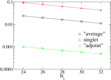
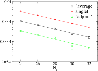
Figure 1: The three different correlation functions Eqs. (3,4), constructed from dressed Polyakov lines, for $r=a$ (left) and $r=4a$ (right); the lines represent single exponential fits.

$r/a$	“average”		$\chi^{2}/{\rm dof}$		singlet		$\chi^{2}/{\rm dof}$		“adjoint”		$\chi^{2}/{\rm dof}$		WL [6]
1	0.	09731(2)	0.	61	0.	09749(1)	0.	26	0.	0925(51)	0.	94	0.	0976(3)
2	0.	1518(7)	0.	51	0.	1526(2)	0.	42	0.	144(6)	0.	56	0.	1529(3)
3	0.	1923(18)	0.	43	0.	1934(11)	1.	07	0.	1865(72)	0.	32	0.	1935(4)
4	0.	2312(83)	1.	13	0.	2286(33)	1.	42	0.	239(25)	0.	98	0.	2280(4)

Table 1: Fitted static potentials $aE_{1}(r)$ from “average”, singlet and “adjoint” correlation functions, as well as the Wilson loop. The values agree within errors.

The result of this procedure for $r/a=1,4$ is shown in Fig. 1, where all three correlation functions are plotted against $N_{t}$. Table 1 shows the resulting slope parameters, the static potentials $E_{1}(r)$, for $r/a=1,2,3,4$. One finds that the potential is the same for all three, and that it corresponds precisely to the zero temperature singlet potential one obtains from a Wilson loop calculation at the same lattice spacing [6].

The matrix elements of the ground states, cf. Eq. (12), are shown in Fig. 2. While our signal gets quickly noisy with growing distance, one can clearly discern that in the “average” channel there is only the trivial constant $1/N^{2}$, in accord with our spectral decomposition. In the singlet channel on the other hand, there is a non-trivial matrix element deviating significantly from one with growing separation, and similarly for the “adjoint” channel.

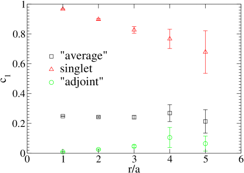
Figure 2: The matrix elements of the ground state in all correlators, Eq. (12).

In the light of this, how can the previous numerical results in the literature be understood? If we just extract the potentials according to the prescription of formulae Eqs. (3,4), we obtain the plot shown in Fig. 3. This indeed reproduces previous results which were suggestive of three different potentials. However, from our analysis it is quite clear that this structure is due to the matrix elements, which get exponentiated when formulae Eqs. (3,4) are used. In order to verify this claim, let us truncate the spectral decompositions of the potentials to the ground state (since we are near the infinite $N_{t}$, or $T=0$ limit),

$${\rm e}^{-V_{{\rm av}}(r)/T} = c^{{\rm av}}_{1}\,{\rm e}^{-E_{1}(r)/T},$$ (21)

$${\rm e}^{-V_{1}(r)/T} = c_{1}^{1}(r)\,{\rm e}^{-E_{1}(r)/T},$$ (22)

$${\rm e}^{-V_{{\rm A}}(r)/T} = c^{{\rm A}}_{1}(r)\,{\rm e}^{-E_{1}(r)/T},$$ (23)

with the same energy $E_{1}(r)$ for all channels, as predicted. Expression (17) for the decomposition of the “average” potential and relation (3) then imply

$$c^{{\rm av}}_{1}=\frac{1}{N^{2}},\qquad c^{{\rm A}}_{1}(r)=\frac{1-c_{1}^{1}(r)}{N^{2}-1}.$$ (24)

Thus, the would-be adjoint and average channel potentials are really given in terms of the singlet static potential $E_{1}(r)$ and its matrix element

$$c^{1}_{1}(r)=\frac{1}{N^{2}}|\langle 1_{\delta\gamma}|\hat{U}_{\gamma\delta}({\bf x},{\bf y})\hat{U}^{{\dagger}}_{\alpha\beta}({\bf x},{\bf y})|1_{\beta\alpha}\rangle|^{2}.$$ (25)

We have inserted the central values of our data for $E_{1}(r),c^{1}_{1}(r)$ in these formulae, Fig. 3, which indeed reproduce the curves extracted by means of the old definition.

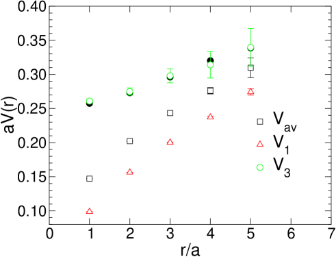
Figure 3: The potentials computed according to Eq. (4). The “adjoint channel” represents a combination of the singlet potential and its matrix element according to Eqs. (23) and (24), which is shown by the full circles.

6 Conclusions

By using projection operators on Hilbert space sectors as well as a numerical analysis of the zero temperature limit, we have shown that Polyakov loop correlators in each of the “average”, singlet and “adjoint” channels defined in the literature receive contributions exclusively from singlet states. Their exponential decay in the temporal direction is thus determined by the singlet potential and its excitations only. As expected, in the zero temperature limit the ground state singlet potential is identical with the one extracted from Wilson loops. Correspondingly, at finite temperature one may extract only a singlet free energy. At fixed lattice spacing, its correct definition as a Boltzmann weighted sum of exponentials without matrix elements follows from Eq. (17) to be

$${\rm e}^{-F_{1}(r)/T}=\sum_{n}{\rm e}^{-E_{n}/T}=\langle{\rm Tr\,}L^{\dagger}({\bf x}){\rm Tr\,}L({\bf y})\rangle.$$ (26)

Any other definition, as well as the other channels considered in the literature, exponentiate (operator dependent) matrix elements, thus faking an $r$ and/or $T$-dependence which is not shared by the physical states.

Finally, let us note that we do not dispute the existence of an adjoint sector, ${\rm F}({\bf x})\otimes\bar{{\rm F}}({\bf y})\otimes{\rm A}({\bf x}_{0})$, in the Hilbert space. However, it is not probed by any combination of Polyakov loops, but requires a different operator, which must not close through the time boundary in order to truly couple to adjoint states. For a non-perturbative investigation, the only way of saturating an open adjoint index is then by a corresponding adjoint source. However, in this case the resulting object is a gluelump formed by an adjoint source coupled to two fundamental ones in the adjoint representation, which is no longer the situation of interest (and considered by perturbation theory), with only two fundamental sources in the adjoint. It appears that more work is needed to resolve these questions.

Note added.

In a somewhat different use of language, it has been suggested to interpret hybrid potentials (i.e. angular momentum excited states with two fundamental sources [17]) as octet potentials, since they appear to approach the gluelump spectrum in the short distance limit [18]. According to their transformation behavior, all these belong to the singlet sector, since the total system of static quark, antiquark and glue is singlet under gauge transformations. While relevant for hybrid mesons, these potentials are therefore not useful for describing intermediate color-charged states as they appear in some nonrelativistic QCD computations [19]. These latter states have to carry an extra adjoint charge. We thank G. Bali for correspondence on this point.

Appendix A Projectors on charge sectors

The transfer matrix $\hat{T}_{0}$ acts on the full Hilbert space of all square integrable wave functions, including ones transforming nontrivially under gauge transformations. This Hilbert space splits into orthogonal sectors with charges in arbitrary representations at any lattice point. These are characterized by their transformation properties under the local gauge group and can be obtained by acting with appropriate projection operators. The projector on gauge-invariant states (with no charges) can be written as

$$\hat{P}=\int Dg\,\hat{R}[g],$$ (27)

where $\hat{R}[g]$ performs a gauge transformation with gauge function $g$, $\hat{R}[g]\psi[U]=\psi[U^{g}]$. Specifically, a string between fundamental charges at ${\bf x},{\bf y}$ transforms as

$$\hat{R}[g]\hat{U}_{\alpha\beta}({\bf x},{\bf y})\hat{R}^{\dagger}[g]=g_{\alpha\gamma}({\bf x})\hat{U}_{\gamma\delta}({\bf x},{\bf y})g^{\dagger}_{\delta\beta}({\bf y})\;.$$ (28)

The projector on states with a fundamental charge at ${\bf x}$ and an anti-fundamental one at ${\bf y}$ is thus given by

$$\hat{P}^{{\rm F}\otimes\bar{{\rm F}}}=N^{2}\int Dg\,{\rm Tr\,}g^{\dagger}({\bf x})\,{\rm Tr\,}g({\bf y})\,\hat{R}[g]\;.$$ (29)

The operator $\hat{P}_{\alpha\beta\mu\nu}^{{\rm F}\otimes\bar{{\rm F}}}$ defined in Eq. (14) maps the component $\psi_{\beta\mu}$ of the representation ${\rm F}\otimes\bar{{\rm F}}$ to the component $\psi_{\alpha\nu}$ and annihilates all other components and charge sectors. The components are here defined by the transformation property

$$\hat{R}[g]\,\psi_{\beta\mu}=\psi_{\gamma\nu}\,g_{\beta\gamma}({\bf x})g^{\dagger}_{\nu\mu}({\bf y})\;.$$ (30)

A direct computation shows

$$\hat{P}_{\alpha\beta\mu\nu}^{{\rm F}\otimes\bar{{\rm F}}}\,\psi_{\gamma\delta}=\frac{1}{N^{2}}\delta_{\beta\gamma}\delta_{\mu\delta}\,\psi_{\alpha\nu}$$ (31)

and that $\hat{P}_{\alpha\beta\mu\nu}^{{\rm F}\otimes\bar{{\rm F}}}$ annihilates all other charge sectors:

$$\hat{P}_{\alpha\beta\mu\nu}^{{\rm F}\otimes\bar{{\rm F}}}\,(1-\hat{P}^{{\rm F}\otimes\bar{{\rm F}}})=0\;.$$ (32)

The normalization of $\hat{P}_{\alpha\beta\mu\nu}^{{\rm F}\otimes\bar{{\rm F}}}$ has conveniently been chosen such that

$$\sum_{\beta\mu}\hat{P}_{\alpha\beta\mu\nu}^{{\rm F}\otimes\bar{{\rm F}}}\,\psi_{\beta\mu}=\psi_{\alpha\nu}\;.$$ (33)

The projection operators $N^{2}\hat{P}_{\alpha\alpha\mu\mu}^{{\rm F}\otimes\bar{{\rm F}}}$ (no sum) provide a decomposition of $\hat{P}^{{\rm F}\otimes\bar{{\rm F}}}$,

$$\hat{P}^{{\rm F}\otimes\bar{{\rm F}}}=N^{2}\sum_{\alpha\mu}\hat{P}_{\alpha\alpha\mu\mu}^{{\rm F}\otimes\bar{{\rm F}}}\;.$$ (34)

References

- [1] G. T. Bodwin, E. Braaten and G. P. Lepage, Phys. Rev. D 51 (1995) 1125 [Erratum-ibid. D 55 (1997) 5853] [arXiv:hep-ph/9407339].
- [2] E. V. Shuryak and I. Zahed, Phys. Rev. D 70 (2004) 054507 [arXiv:hep-ph/0403127].
- [3] L. S. Brown and W. I. Weisberger, Phys. Rev. D 20 (1979) 3239.
- [4] L. D. McLerran and B. Svetitsky, Phys. Rev. D 24 (1981) 450.
- [5] S. Nadkarni, Phys. Rev. D 34 (1986) 3904.
- [6] O. Philipsen, Phys. Lett. B 535 (2002) 138 [arXiv:hep-lat/0203018].
- [7] A. Nakamura and T. Saito, Prog. Theor. Phys. 111 (2004) 733 [arXiv:hep-lat/0404002]; O. Kaczmarek, F. Karsch, P. Petreczky and F. Zantow, Phys. Lett. B 543 (2002) 41 [arXiv:hep-lat/0207002]; S. Digal, S. Fortunato and P. Petreczky, Phys. Rev. D 68 (2003) 034008 [arXiv:hep-lat/0304017].
- [8] V. A. Belavin, V. G. Bornyakov and V. K. Mitrjushkin, Phys. Lett. B 579 (2004) 109 [arXiv:hep-lat/0310033].
- [9] P. de Forcrand and O. Philipsen, Phys. Lett. B 475 (2000) 280.
- [10] M. Creutz, Phys. Rev. D 15 (1977) 1128.
- [11] M. Lüscher, Commun. Math. Phys. 54 (1977) 283.
- [12] J. B. Kogut and L. Susskind, Phys. Rev. D 11 (1975) 395.
- [13] M. Luscher and P. Weisz, JHEP 0207 (2002) 049 [arXiv:hep-lat/0207003] and references therein.
- [14] O. Kaczmarek, F. Karsch, E. Laermann and M. Lutgemeier, Phys. Rev. D 62 (2000) 034021 [arXiv:hep-lat/9908010]; M. Laine and O. Philipsen, Phys. Lett. B 459 (1999) 259 [arXiv:hep-lat/9905004]; A. Hart, M. Laine and O. Philipsen, Nucl. Phys. B 586 (2000) 443 [arXiv:hep-ph/0004060]; S. Datta and S. Gupta, Nucl. Phys. B 534 (1998) 392 [arXiv:hep-lat/9806034].
- [15] S. Nadkarni, Phys. Rev. D 33, 3738 (1986).
- [16] O. Philipsen, M. Teper and H. Wittig, Nucl. Phys. B 469 (1996) 445 [arXiv:hep-lat/9602006].
- [17] K. J. Juge, J. Kuti and C. J. Morningstar, Nucl. Phys. Proc. Suppl. 63 (1998) 326 [arXiv:hep-lat/9709131].
- [18] G. S. Bali and A. Pineda, Phys. Rev. D 69 (2004) 094001 [arXiv:hep-ph/0310130]; N. Brambilla, A. Pineda, J. Soto and A. Vairo, Nucl. Phys. B 566 (2000) 275 [arXiv:hep-ph/9907240].
- [19] P. L. Cho and A. K. Leibovich, Phys. Rev. D 53 (1996) 150 [arXiv:hep-ph/9505329].