Solar Neutrinos Before and After Neutrino 2004

Abstract:

We compare, using a three neutrino analysis, the allowed neutrino oscillation parameters and solar neutrino fluxes determined by the experimental data available Before and After Neutrino 2004. New data available after Neutrino 2004 include refined KamLAND and gallium measurements. We use six different approaches to analyzing the KamLAND data. We present detailed results using all the available neutrino and anti-neutrino data for $\Delta m^{2}_{21}$, $\tan^{2}\theta_{12}$, $\sin^{2}\theta_{13}$, and $\sin^{2}\eta$ (sterile fraction). Using the same complete data sets, we also present Before and After determinations of all the solar neutrino fluxes (which are treated as free parameters), an upper limit to the luminosity fraction associated with CNO neutrinos, and the predicted rate for a ⁷Be solar neutrino experiment. The $1\sigma$ ($3\sigma$) allowed range of $\Delta m^{2}_{21}=8.2^{+0.3}_{-0.3}(^{+{1.0}}_{{-0.8}})\times 10^{-5}\,{\rm eV^{2}}$ is decreased by a factor of 1.7 (5), but the allowed ranges of all other neutrino oscillation parameters and neutrino fluxes are not significantly changed. Maximal $\theta_{12}$ mixing is disfavored at 5.8$\sigma$ and the bound on the mixing angle $\theta_{13}$ is slightly improved to $\sin^{2}\theta_{13}<0.048$ at 3$\sigma$. The predicted rate in a ⁷Be neutrino-electron scattering experiment is $0.665\pm 0.015\,(^{+0.045}_{-0.040})$ of the rate implied by the BP04 solar model in the absence of neutrino oscillations. The corresponding predictions for $p-p$ and $pep$ experiments are, respectively, $0.707^{+0.011}_{-0.013}(^{+0.041}_{-0.039})$ and $0.644^{+0.011}_{-0.013}(^{+0.045}_{-0.037})$. In order to clarify what measurements constrain which parameters best, we also analyze the solar neutrino data separately and the reactor anti-neutrino data separately, both Before and After Neutrino 2004. We derive upper limits to CPT violation in the weak sector by comparing reactor anti-neutrino oscillation parameters with neutrino oscillation parameters. We also show that the recent data disfavor at 91% CL a proposed non-standard interaction description of solar neutrino oscillations. We have verified that our results are insensitive (changes much less than $1\sigma$) to which of six approaches we use in analyzing the KamLAND data, which of the published ⁸B neutrino energy spectra we adopt, and the precise value of the gallium solar neutrino event rate.

1 Introduction

How have the recently released data from the the KamLAND reactor anti-neutrino experiment [1] and the revised average gallium solar neutrino rate [2, 3, 4, 5] improved our knowledge of neutrino properties and of solar neutrino fluxes?

We concentrate in this paper on a Before-After comparison that is made possible by the new data released at Neutrino 2004 (Paris, June 19–24, 2004). We determine how the new KamLAND and solar neutrino data affect our knowledge of the parameters that characterize solar neutrino oscillations [$\Delta m^{2}_{21}$, $\theta_{12}$, $\theta_{13}$, $\eta_{\rm sterile}$] and the parameters that characterize solar energy generation and neutrino fluxes [$L_{\rm CNO}$, $\phi(p-p)$, $\phi(^{7}{\rm Be})$, $\phi(^{8}{\rm B})$, $\phi(^{13}{\rm N})$, $\phi(^{15}{\rm O})$, and $\phi(^{17}{\rm F})$].

In order to clarify which measurements constrain what quantities and by how much, we analyze the reactor data [1, 6, 7] separately and the solar neutrino data [2, 3, 4, 5, 8, 9, 10, 11, 12, 13, 14] separately. We use six different approaches to analyzing the KamLAND data (see section 3.2) in order to assess the quantitative importance, or lack of importance, of different analysis procedures.

The conventional wisdom is that a quantitative improvement in our knowledge of neutrino parameters and solar neutrino fluxes is all that we should expect. According to this view, the existing solar neutrino experiments have reached a level of maturity and precision at which new data from these operating experiments are expected to lead to refinements, but not revolutions. This conventional wisdom could be wrong and sub-dominant contributions due, for example, to non-standard interactions [15, 16], to sterile neutrinos [17, 18], or even to CPT violation [19] could show up in the operating experiments. We investigate all these possibilities.

We analyze the experimental data assuming that vacuum and matter neutrino oscillations [20, 21] occur among three active neutrino species (with the possibility also of oscillation to a sterile neutrino [22]). The techniques that we use in this analysis have been described previously in a series of papers, especially refs. [23, 24, 25]. Many other groups have reported analyses of solar neutrino and reactor data, see ref. [26], but our analysis is unique so far-we believe-in treating all of the solar neutrino fluxes as free parameters, subject only to the luminosity constraint, refs. [27, 28] (i.e., essentially energy conservation).

Our principal results are shown in figure 1 and figure 2 and in table 2 and table 3.

We begin by discussing in section 2 the experimental data and the $\chi^{2}$ formulations we use for different applications. The data are summarized in table 1. We then present in section 3 the results of our reactor-only analyses: the allowed regions in neutrino oscillation space that are compatible with the reactor data available Before Neutrino 2004 and the reactor data (notably the new KamLAND data [1]) available After Neutrino 2004. We also describe in section 3 the six different approaches we use in analyzing the KamLAND data and summarize the technical aspects of our KamLAND analyses. Next we present in section 4 the results of our solar-only analyses: the allowed regions in neutrino parameter space and neutrino fluxes that are compatible with all solar neutrino data available both Before and After Neutrino 2004. Figure 1 summarizes the results of our Before-After reactor-only and solar-only comparisons.

We present in section 5 and in table 2 and table 3 the results of our global three neutrino analyses of solar neutrino experimental results and reactor anti-neutrino data. We give the best-estimates and the uncertainties for neutrino oscillation parameters and for solar neutrino fluxes. We also determine in this section the upper bound on the sterile neutrino flux and on the luminosity of the Sun that is associated with the CNO nuclear fusion reactions. We compare in section 7 the allowed oscillation regions of rector anti-neutrinos with the allowed oscillation regions of solar neutrinos in order to establish an upper limit on CPT violation in the weak sector. We summarize and discuss our main results in section 8. In the Appendix, we present some details of the analysis involving $\theta_{13}$.

2 Experimental data and $\chi^{2}$

Table 1: Experimental data. We summarize the solar, reactor, accelerator, and atmospheric data used in our global analyses. Only experimental errors are included in the column labelled Result/SM. Here the notation SM corresponds to predictions of the Bahcall-Pinsonneault standard solar model (BP04) of ref. [31] and the standard model of electroweak interactions [32] (with no neutrino oscillations). The new average gallium rate is $68.1\pm 3.75$ SNU (see ref. [2]). The SNO rates (pure $D_{2}O$ phase) in the column labelled Result/SM are obtained from the published SNO spectral data by assuming that the shape of the ${\rm{}^{8}B}$ neutrino spectrum is not affected by physics beyond the standard electroweak model. However, in our global analyses, we allow for spectral distortion. The SNO rates (salt phase) are not constrained to the ⁸B shape [12]. The K2K and atmospheric data are used only in the analysis of $\theta_{13}$, which is discussed in Appendix A.

Experiment	Observable ($\#$ Data)	Measured/SM	Reference
Chlorine	Average Rate (1)	[CC]=$0.30\pm 0.03$	[8]
SAGE+GALLEX/GNO†	Average Rate (1)	[CC]=$0.52\pm 0.03$	[3, 4, 5]
Super-Kamiokande	Zenith Spectrum (44)	[ES]=$0.406\pm 0.013$	[10]
SNO (pure $\rm D_{2}$O phase)	Day-night Spectrum (34)	[CC]=$0.31\pm 0.02$	[13, 14]
		[ES]=$0.47\pm 0.05$	[13, 14]
		[NC]=$1.01\pm 0.13$	[13, 14]
SNO (salt phase)	Average Rates (3)	[CC]=$0.28\pm 0.02$	[12]
		[ES]=$0.38\pm 0.05$	[12]
		[NC]=$0.90\pm 0.08$	[12]
KamLAND	Spectrum (10)	[CC]=$0.69\pm 0.06$	[6]
CHOOZ	Spectrum (14)	[CC] = $1.01\pm 0.04$	[7]
K2K	Spectrum (6)	[CC]$(\nu_{\mu})$ = $0.70^{+0.11}_{-0.10}$	[29]
Atmospheric	Zenith Angle Distributions (55)	[0.5-1.0]	[30]

^† SAGE rate: $66.9\pm 3.9\pm 3.6$ SNU [3]; GALLEX/GNO rate: $69.3\pm 4.1\pm 3.6$ SNU [4, 5].

We summarize in this section the experimental data we use and the $\chi^{2}$ distributions that we analyze.

Table 1 summarizes the solar [2, 3, 4, 5, 8, 13, 14], reactor [1, 6, 7], and atmospheric [30] data used in our global analyses that are presented in section 5. The number of data derived from each experiment are listed (in parentheses) in the second column of the table. In the third column, labelled Measured/SM, we list for each experiment the quantity Measured/SM, the measured total rate divided by the rate that is expected assuming the correctness of, as relevant, the standard solar model and the standard model of electroweak interactions (i.e., no neutrino oscillations or other non-standard physics).

We calculate the global $\chi^{2}$ by fitting to all the available data, solar plus reactor. For the analysis of the upper bound on $\theta_{13}$, we also include data from the K2K accelerator experiment and from atmospheric measurements, see eq. (28). Formally, the global $\chi^{2}$ can be written in the form [33, 34]

$$\chi^{2}_{\rm global} = \chi^{2}_{\rm solar}(\Delta m^{2}_{21},\theta_{12},\theta_{13},\{f_{\rm B},f_{\rm Be},f_{p-p},f_{\rm CNO}\})$$ (1)

$$+ \chi^{2}_{\rm KamLAND}(\Delta m^{2}_{21},\theta_{12},\theta_{13})\,.$$

Depending upon the case we consider, there can be as many as nine free parameters in $\chi^{2}_{\rm solar}$, including, $\Delta m^{2}_{21},\theta_{12}$, $\theta_{13}$ , $f_{\rm B},$ $f_{\rm Be}$, $f_{p-p}$, and $f_{\rm CNO}$ (3 CNO fluxes, see below). The neutrino oscillation parameters $\Delta m^{2}_{21},\theta_{12},\theta_{13}$ have their usual meaning. The reduced fluxes $f_{\rm B}$, $f_{\rm Be}$, $f_{p-p}$, and $f_{\rm CNO}$ are defined as the true solar neutrino fluxes divided by the corresponding values of the fluxes predicted by the BP04 standard solar model [31]. We extend in section 5.2 the formalism to include sterile neutrinos.

The function $\chi^{2}_{\rm KamLAND}$ depends only on $\Delta m^{2}_{21}$, $\theta_{12}$ and $\theta_{13}$.

We marginalize $\chi^{2}_{\rm global}$ making use of the function $\chi^{2}_{\rm CHOOZ+ATM+K2K}(\theta_{13})$ that was obtained following the analysis of ref. [35] of atmospheric [30], K2K accelerator [29], and CHOOZ reactor [7] data (see also, refs. [36, 37]). We have not assumed, as is often done, a flat probability distribution for all values of $\theta_{13}$ below the CHOOZ bound. The fact that we take account of the actual experimental constraints on $\theta_{13}$ decreases the estimated influence of $\theta_{13}$ compared to what would have been obtained for a flat probability distribution.

3 Reactor data

We compare in section 3.1 the allowed oscillation regions for $\Delta m^{2}_{21}$, $\tan^{2}\theta_{12}$, and $\sin^{2}\theta_{13}$ that are determined from the first KamLAND results [6], together with the CHOOZ data [7], with the oscillation regions determined by including the recently released new KamLAND data [1]. This Before-After comparison is illustrated in the two right-hand panels of figure 1. We also show in section 3.1 that the new KamLAND data more strongly disfavor a proposed [15] non-standard description of solar neutrino oscillations.

We describe in section 3.2 six different sets of assumptions that were used in analyzing the KamLAND data. We then discuss in section 3.3 some technical aspects of the analysis of the second release of KamLAND data.

All of the neutrino properties and the solar neutrino fluxes that are determined in section 5 are robust with respect to the six different analysis approaches described in section 3.2.

3.1 Allowed regions: KamLAND reactor data

In this subsection, we discuss briefly in section 3.1.1 the implications of the spectral distortion observed recently by the KamLAND collaboration, and then in section 3.1.2 present the best-fit values for neutrino parameters and their uncertainties, as well as the allowed contours obtained using the new KamLAND data. We show in section 3.1.3 that the new KamLAND data more strongly disfavor a previously proposed description of solar neutrino oscillations in terms of non-standard interactions.

3.1.1 Spectral distortion

The new KamLAND data [1] confirm the expected deficit of $\overline{\nu}_{e}$ due to oscillations with parameters in the LMA region. More importantly, the new data show the expected distortion of the energy spectrum. In their new paper [1] , the KamLAND collaboration report a goodness-of-fit test for a scaled no-oscillation energy spectrum with the normalization fitted to the data. They find a goodness-of-fit of only 0.1%. We confirm that the hypothesis of an undistorted scaled spectrum can fit the data with less than 0.2% probability.

As a consequence, the 3$\sigma$ region from the After KamLAND-only analysis shown in the lower right hand panel of figure 1 does not extend to mass values larger than $\Delta m^{2}_{21}=2\times 10^{-4}$ eV². For the now-excluded large $\Delta m^{2}_{21}$ values, the predicted spectral distortions are too small to fit the KamLAND data.

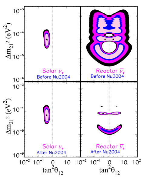
Figure 1: Allowed oscillation parameters: Solar vs KamLAND. The two left panels show the 90%, 95%, 99%, and 3$\sigma$ allowed regions for oscillation parameters that are obtained by a global fit of all the available solar data [8, 3, 4, 10, 13, 14, 5, 12]. The two right panels show the 90%, 95%, 99%, and 3$\sigma$ allowed regions for oscillation parameters that are obtained by a global fit of all the reactor data from KamLAND and CHOOZ [6, 7]. The two upper (lower) panels correspond to the analysis of all data available before (after) the Neutrino 2004 conference, June 14-19, 2004 (Paris). The new KamLAND data [1] are sufficiently precise that matter effects discernibly break the degeneracy between the two mirror vacuum solutions in the lower right panel.

3.1.2 KamLAND-only: best-fit values, uncertainties, and allowed regions

Figure 1 compares the allowed regions for anti-neutrinos as determined by the KamLAND reactor experiment before Neutrino 2004 (upper right panel) with the allowed regions after Neutrino 2004 (lower right panel). The two panels in the right column of figure 1 represent the Before-After summary of the effect of the new KamLAND data released at Neutrino 2004.

Before Neutrino 2004, the best-fit solutions for the reactor data were $\Delta m^{2}_{21}=7.1\times 10^{-5}\,{\rm eV^{2}}$ and $\tan^{2}\theta_{12}=0.52\,\&\,1.9\,$ (see ref. [23]). Within the statistical precision of the first KamLAND data, matter effects were too small to provide a meaningful discrimination between the two octants for $\theta_{12}$.

After Neutrino 2004, the best-fit values ($\chi^{2}=12.5$) is shown in the lower panel of figure 1 and is:

$$\Delta m^{2}_{21}=8.3^{+0.40}_{-0.30}(^{+{1.2}}_{{-1.0}})\times 10^{-5}\,{\rm eV^{2}},\,\,{\tan^{2}\theta_{12}}=0.36^{+0.10}_{-0.08}(^{+6.2}_{-0.2})\,({\rm reactor~{}data:After}).$$ (2)

As pointed out in Ref. [23], matter effects, although small, cannot be neglected in the analysis of precise KamLAND data [1]. In the analysis of the currently available data, matter effects break the degeneracy between the two octants of the mixing angle and induce an extra $\Delta\chi^{2}=0.2$ for what would otherwise be (in the absence of matter effects) the mirror minimum at $\tan^{2}\theta_{12}=2.7$.

We describe in section 3.2 six different approaches to analyzing the KamLAND data. The uncertainties shown in eq. (2) are $1\sigma$ ($3\sigma$) errors for KamLAND analysis option number 3 of section 3.2.

The best-fit values and uncertainties of $\Delta m^{2}_{21}$ and $\tan^{2}\theta_{12}$ are essentially independent of the six analysis options for KamLAND data. The best-fit value for $\Delta m^{2}_{21}$ is the same to the numerical accuracy of eq. (2) for all six analysis options and the range of the $1\sigma$ uncertainty varies by only about $\pm 0.15\sigma$. The best-fit value of $\tan^{2}\theta_{12}$ varies by about $\pm 0.2\sigma$ and the range of the $1\sigma$ uncertainty varies by $\pm 0.1\sigma$.

Our results are in good agreement with those obtained by the KamLAND collaboration. They report a best fit point at $\Delta m^{2}_{21}=8.3\times 10^{-5}\,{\rm eV^{2}}$ and $\tan^{2}\theta_{12}=0.41$, which is within the range of the best fit points obtained with our six analysis procedures and almost identical to our preferred best-fit point. Comparing the results of our binned analysis with the results of the event-by-event maximum likelihood analysis of KamLAND, we find only two “barely visible” differences: (i) the lower ”island” is allowed at a slightly lower CL in all of our binned analyses; (ii) the CL at which the ”best-fit island” extends into maximal mixing is below 95% CL in Ref. [1], while in our binned analysis we find maximum mixing is slightly above or below 95% CL depending on the particular analysis option we adopt.

The new KamLAND data [1], together with the CHOOZ [7], K2K [29], and atmospheric [30] results, lead to the following allowed range of $\sin^{2}\theta_{13}$,

$$\sin^{2}\theta_{13}=0.005^{+0.011}_{-0.005}(^{+0.045}_{-0.005})\,.$$ (3)

For the six different analysis options discussed in section 3.2, the best-fit value of $\sin^{2}\theta_{13}$ varies by less than $\pm 0.1\sigma$ and the range of the $1\sigma$ uncertainty varies by $\pm 0.1\sigma$. Note, however, that the best-fit value of $\sin^{2}\theta_{13}$ is not significantly different from zero.

3.1.3 Non-standard interaction

Non-standard flavor-changing neutrino-matter interactions could potentially play a profound role in solar neutrino oscillations, even if the non-standard interactions are much weaker than standard weak interactions. In ref. [15], Friedland, Lunardini, and Peña-Garay proposed a non-standard description of solar neutrino and reactor oscillations that expanded the allowed regions for neutrino oscillation parameters beyond what was allowed by standard interactions. The preferred oscillation parameters for this non-standard interaction are:

$$\Delta m^{2}_{21}=1.5\times 10^{-5}\,{\rm eV^{2}},\,\,\tan^{2}\theta_{12}=0.39\ ({\rm non-standard~{}interactions:ref.~{}\cite[cite]{[\@@bibref{}{nsi}{}{}]}}).$$ (4)

After the new KamLAND measurements, this solution is disfavored at the 91% CL for 2 dof. This is a significant improvement over the first KamLAND results, which disfavored at 78% CL the non-standard solution of eq. (4).

3.2 Six methods of analyzing KamLAND data

We have analyzed the new KamLAND data with six different approaches. We first enumerate the six sets of assumptions that were used and then comment on the differences between the various assumptions. We provide additional technical details in the following subsection, section 3.3.

1. Poisson statistics, our normalization, 13 energy bins

2. Poisson statistics, KamLAND normalization, 13 energy bins

3. Poisson statistics, our normalization, 9+1 energy bins

4. Poisson statistics, KamLAND normalization, 9+1 energy bins

5. Gaussian statistics,our normalization,9+1 energy bins

6. Gaussian statistics, KamLAND normalization, 9+1 energy bins

We prefer to combine the four highest energy bins of the KamLAND, which have only 6 events in total, in order to reduce the fluctuations and to make the analysis more stable. In order to verify that this additional binning does not affect the final results, we performed separate analyses with the full 13 published KamLAND energy bins (1 and 2 above) and with 9 + 1 energy bins (3, 4, 5, and 6). As we shall see in section 3.3, our best-fit normalization for the number of observed events agrees with the best-fit normalization of KamLAND but the two normalizations differ slightly (by less than $1\sigma)$. We have therefore performed analyses with our normalization (1, 3, and 5 above) and separately with the KamLAND normalization (2, 4, and 6). Finally, we have compared, with the same energy binning and normalization, the results obtained with Poisson statistics (item 3) with the results obtained with Gaussian statistics (item 5).

Of the six possibilities listed above, we prefer number 3. This option relies totally on our own calculations, so it is an independent check of the calculations of the KamLAND collaboration [1]. Moreover, option 3 minimizes the effects of fluctuations due to low statistics bins.

Fortunately, we shall show in section 5 that the globally-inferred results for neutrino parameters and solar neutrino fluxes are essentially independent of which one of the six options we choose. We have already seen in section 3.1 that all six of the analysis options yield consistent results to an accuracy of much better than $1\sigma$.

3.3 Some technical details: reactor anti-neutrino analysis

The present analysis is based on data taken from 9 March, 2002 through 11 January, 2004 [1]. We take account of corrections due to, among other things, the spallation cut and the detection efficiency of the tagged signal of electron antineutrinos (see ref. [1]). We assume a time independent correction due to maintenance and bad runs and normalize our results after fiducial cuts to the KamLAND total exposure of 766.3 ton$\cdot$year.

We included in our calculations the time dependences due to the turn on/off of the different reactors in Japan. We have tracked the power of Japanese reactors on $\rm http://www.fepc-atomic.jp/public_{i}nfo/unten/index.html$; the web page is owned by The Federation of Electric Power Companies of Japan. At present, this Web page tabulates the operational days of the 52 Japanese reactors up to June 2003. Furthermore, we have also been tracking the reactor power on a weekly basis since April 2003. This information allowed us to account for the time variations of the power-averaged antineutrino baseline, which can be as large as 20% (in good agreement with the results presented by KamLAND [1]). Other time dependences like variations of the reactor composition could not be tracked, but have been shown to be small [38]. We use the time averaged fuel compositions ²³⁵U: ²³⁸U: ²³⁹Pu: ²⁴¹Pu = 0.568: 0.078 : 0.297: 0.057. Non-Japanese reactors contribute to the KamLAND signal less than 3% and their flux contribution is assumed time independent.

With all this information, we find that, in the absence of oscillations, the expected number of antineutrino events above 2.6 MeV energy threshold is 381 which is in good agreement with the KamLAND estimate of $365.2\pm 23.7({\rm syst})$. All of the solar neutrino parameters we infer from a global solution of the solar plus reactor data are, to high accuracy (much better than $1\sigma$) independent of which normalization we adopt (see items 1 and 2, items 3 and 4, and items 5 and 6 of section 3.2 and the discussion of the results all six analysis approaches in section 5).

We analyze the KamLAND energy spectrum by making a $\chi^{2}$ fit to their binned energy spectrum. The KamLAND spectrum contains a total of 13 energy bins above 2.6 MeV, with only 6 events in the four highest energy bins. In order to reduce the fluctuations associated with the small number of events in these four bins, we combine for options 3, 4, 5, and 6 of section 3.2 the data of these high energy events into a single bin with $E>6$ MeV (containing 6 events). For this 10 bin analysis, we compute the results assuming that the binned data is Poisson distributed,

$$\chi^{2}_{\rm KamLAND}~{}=~{}{\rm min}_{\alpha}\sum_{i=1}^{10}\left[2(\alpha R^{i}_{\rm th}-R^{i}_{\rm exp})+2R^{i}_{\rm exp}\ln\left(\frac{R^{i}_{\rm exp}}{\alpha R^{i}_{\rm th}}\right)\right]+\frac{(\alpha-1)^{2}}{\sigma_{\rm sys}^{2}}\;,$$ (5)

or that the binned data is Gaussian distributed,

$$\chi^{2}_{\rm KamLAND}~{}=~{}{\rm min}_{\alpha}\sum_{i=1}^{10}\frac{(\alpha\,R_{\rm th}^{i}-R_{\rm exp}^{i})^{2}}{\sigma^{2}_{\rm stat,i}}+\frac{(\alpha-1)^{2}}{\sigma^{2}_{\rm syst}}$$ (6)

with $\sigma^{2}_{\rm stat,i}=R_{\rm exp}^{i}$. We also use a $\chi^{2}$ completely analogous to eq. (5) when analyzing all 13 energy bins (options 1 and 2 of section 3.2).

In eqs. (5) and (6), $\alpha$ is an absolute normalization constant and $\sigma_{\rm syst}=6.5\%$ is the total systematic uncertainty from several theoretical and experimental sources (see table I of ref. [1]). In our binned analysis we have neglected the shape distortion errors. Using the presently available information we have been able to compute the shape distortion errors due to the uncertainties in the energy scale and reactor $\overline{\nu}_{e}$ spectra and found them to be $<0.8\%$ and $<0.5\%$ respectively in any of the bins. We include in $R_{\rm th}^{i}$ the expected number of events in the presence of oscillations, including the backgrounds from accidental coincidences ($2.69\pm 0.02$ events) and spallation sources ($4.8\pm 0.9$ events). The accidental background contributes to the event rate in the first bin while the spallation background is distributed among all the energy bins and peaks at $E\sim 5.6$ MeV.

Our statistical analysis is different from the one of the KamLAND collaboration. First, we include the effect of $\theta_{13}$ as described in Sec. A. Second, KamLAND collaboration performs an unbinned maximum likelihood fit. Such an event-by-event likelihood analysis provides a more powerful tool to extract information from the data (see for instance Ref.[39]). At the moment, only the KamLAND collaboration can perform an eventy-by-event maximum likelihood fit since to do so requires knowing the antineutrino energy (and time) for each event, which is not publicly available.

In our previous studies [23, 25, 33, 34], we used a calculational grid of 80 points per decade of $\Delta m_{21}^{2}$ and 80 points per decade of $\tan^{2}\theta_{12}$. The previous grid is not sufficiently dense to take full account of the accuracy in the currently available neutrino data. Hence we are now using throughout the present paper a grid of 180 points for each decade of $\Delta m_{21}^{2}$, 180 points for each decade of $\tan^{2}\theta_{12}$, and a step size of 0.00125 for $\sin^{2}\theta_{13}$.

As mentioned before, matter effects cannot be neglected in the present analysis of KamLAND data. They are most important in the lowest island and slightly favor the light versus the dark side of the mixing angle. To estimate the size of matter effects in the present analysis we define, $F({\rm matter~{}vs~{}vacuum})$, as the fractional difference in the event rate for the KamLAND detector calculated with and without including matter effects in the Earth. We find that, within the $1\sigma(3\sigma)$ allowed region of the analysis of the KamLAND energy spectrum, the maximum value of $|F({\rm matter~{}vs~{}vacuum})|$ corresponds to $0.4$% ($2.3$%). The maximum change in $\chi^{2}$ due to including matter effects in the KamLAND-only analysis is 0.5 (1.4) at $1\sigma(3\sigma)$.

4 Solar neutrino analysis

In this section, we compare the allowed oscillation regions determined from all previous solar neutrino experiments (chlorine, Kamiokande, SAGE, GALLEX/GNO, Super-Kamiokande, SNO) [3, 4, 5, 8, 9, 10, 12, 13, 14] with the oscillation regions determined by including the slightly revised average gallium rate released at Neutrino 2004 [2] with the previously available data.

We present in section 4.1 the main scientific results of this solar-only analysis . In section 4.2, we describe some technical details of our analysis of the solar neutrino data.

4.1 Allowed regions: solar neutrinos

How much have the new solar neutrino data changed the allowed regions? The answer is ’imperceptibly’, as the reader can easily see by comparing the upper left panel of figure 1 with the lower right panel of figure 1. We challenge even the most sharp eyed of our colleagues to discern the difference.

Figure 1 shows the allowed regions for all solar neutrino experiments before Neutrino 2004 (upper left panel) with the allowed regions after Neutrino 2004 (lower left panel). The two panels in the left column of figure 1 represent the Before-After summary of the effect of the new SNO data released at Neutrino 2004.

The allowed regions for solar neutrino oscillations presented in figure 1 are somewhat larger than the regions obtained by other authors [26]. The reason is that we have allowed all of the neutrino fluxes to be free parameters subject only to the luminosity constraint [27], which is equivalent to energy conservation if light element fusion is the source of the solar luminosity. Most other groups [26] incorporate in their analysis the solar neutrino fluxes and their uncertainties that are predicted by the standard solar model [31, 40].

One can give good arguments for either including, or not including, the predicted solar model fluxes in the phenomenological analysis. The sound velocities measured from helioseismology are in excellent agreement with the standard solar model predictions [40, 41] and the SNO measurement of the total ⁸B neutrino flux [12, 13] is also in agreement with the solar model predictions. These confirmations of the solar model justify the inclusion of the solar model predictions either as priors or as part of the $\chi^{2}$ analysis.

We prefer instead to allow all of the solar neutrino fluxes to be free parameters in order to separate cleanly the astronomy from the neutrino physics. However, we have calculated the allowed ranges of neutrino oscillation parameters and neutrino fluxes both ways, including the solar model predictions and letting all the neutrino fluxes be free parameters. Both methods yield similar–but not identical–results for $\Delta m^{2}_{21}$ and $\tan^{2}\theta_{12}$, although the method with free fluxes and the luminosity constraint yields a more accurate determination of the $p-p$ solar neutrino flux [25].

4.2 Some technical details: solar neutrino analysis

Details of our solar neutrino analyses have been described in previous papers [23, 24, 25]. The solar neutrino data we use are described in table 1. Solar data includes the Gallium (1 data point) and Chlorine (1 data point) radiochemical rates, the Super-Kamiokande zenith spectrum (44 bins), and SNO data previously reported for phase 1 and phase 2. The SNO data set available so far consists of the total day-night spectrum measured in the pure D₂O phase (34 data points), plus the total charged current (CC, 1 data point), electron scattering (ES, 1 data point), and neutral current (NC, 1 data point) rates measured in the salt phase [12, 13, 14]. We use for the radiochemical experiments the neutrino absorption cross sections given in refs. [42, 43].

We discuss in section 4.2.1 our treatment of solar neutrino fluxes. We discuss in section 4.2.2 how the choice of different available determinations of the shape of the ⁸B neutrino energy spectrum affects the neutrino parameters and solar neutrino fluxes that are inferred using the existing solar neutrino and reactor anti-neutrino data.

4.2.1 Treatment of solar neutrino fluxes

Total neutrino fluxes are not required in our analysis and we only use the model fluxes to make dimensionless the neutrino flux output of our analysis. We express all neutrino fluxes determined by our phenomenological analysis of experimental data as ratios of the measured to the predicted (by the standard solar model BP04, [31]) neutrino fluxes. As a result of an obsessive sense for precision, we have used the most up-to-date electron and neutron densities and distributions of neutrino fluxes that are available on http:/www.sns.ias.edu/ jnb. We have checked, however, that none of our conclusions are affected significantly ($<$0.5%) by the particular choice of profiles we adopt. We have used solar models available at http:/www.sns.ias.edu/$\sim$jnb from 2004, 2000, 1998, and 1995. Within the accuracy of the parameter determinations and the published grid sizes of the models, our inferences about neutrino parameters are unaffected by the choice of profile. All of the profiles are essentially unchanged to the accuracy of interest for solar neutrino work by the improvements in the models over time (although the grid size has increased monotonically since 1962). We may regard the temperature and density profiles as experimentally confirmed because of the remarkable agreement between standard solar model predictions and helioseismological measurements [40, 41].

All neutrino oscillation parameters and neutrino fluxes are treated as free parameters. We obtain the allowed ranges of a particular parameter, solar or neutrino, by marginalizing the $\chi^{2}$ over all other parameters. In the $\chi^{2}$ analysis, the SNO and Super-Kamiokande sectors are correlated by the theoretical ⁸B spectrum.

4.2.2 Sensitivity to ⁸B neutrino spectrum

In our previous global studies of solar neutrino and reactor anti-neutrinos, we have used the Ortiz et al. [44] central values of the ⁸B neutrino energy spectrum and the Bahcall et al. errors [42] on the energy spectrum. And, indeed, we used this prescription in all of the initial calculations in this paper.

Recently, however, Winter et al. [45] have redetermined the ⁸B neutrino spectrum from new measurements of the $\alpha$ energy spectrum following the $\beta^{+}$ decay of ⁸B. We have redone our three neutrino analyses replacing the Ortiz el al. central values of the ⁸B neutrino spectrum by the Winter et al. central values. We find that the Gallium and Chlorine rates are shifted downward by less than 0.1 $\sigma$. For ⁸B neutrinos, the charged current and neutral current rates on ${\rm D_{2}O}$, as well as the $\nu-e$ scattering rate, are shifted downward by less than $0.1\sigma$, $0.3\sigma$, and $0.1\sigma$, respectively. The higher energy bins of the charged current and the electron scattering spectrum can be shifted downward by less than or equal to 5%. With the current state of the solar neutrino measurements, all of these changes are small compared to the uncertainties that result from a $1\sigma$ shift in the experimental (electron) energy scale (up to 20% at $1\sigma$) and energy resolution errors (up to 16% at $1\sigma$).

We have verified that the values of neutrino parameters and the values of neutrino fluxes derived in this paper from the different analyses are, to the accuracy we quote the numbers, independent of whether we use the Ortiz et al. ⁸B neutrino energy spectrum or the Winter et al. energy spectrum. We have also verified that our results are unchanged to the quoted numerical accuracy if we use the Winter et al. error estimate on the shape of the energy spectrum or the more conservative Bahcall et al. error estimate.

5 New global solution: solar plus reactor data

In this section, we present the results of a global analysis of all the available solar and reactor data. We use the data summarized in table 1 and the total $\chi^{2}_{\rm global}$ defined by eq. (1). We marginalize $\chi^{2}_{\rm global}$ with respect to $\theta_{13}$ by making use of the function $\chi^{2}_{\rm CHOOZ+ATM+K2K}(\theta_{13})$ that is obtained from an analysis of atmospheric [30], K2K accelerator  [29], and CHOOZ reactor [7] data (see Appendix for details).

We begin in section 5.1 by presenting the solar neutrino oscillation parameters that are allowed Before and After Neutrino 2004 by the totality of existing neutrino data. We then summarize in section 5.3 the allowed ranges of solar neutrino fluxes.

5.1 Neutrino oscillation parameters: best-fit values, uncertainties, and independence of analysis method

Table 2: Global allowed regions. The table presents the best-fit oscillation parameters and the 1$\sigma$ (3$\sigma$) ranges determined from solar and reactor data available Before Neutrino 2004 (top row) and After Neutrino 2004 (bottom row). We have included the results of the marginalized $\chi^{2}$ distributions for $\theta_{13}$ derived from the analysis of Atmospheric, K2K and CHOOZ data  [36]. The quantity $\sin^{2}\eta$ characterizes the sterile fraction (see ref. [23, 25] and the discussion in section 5.2). The table presents the value obtained when all of the solar neutrino fluxes are treated as free parameters and the luminosity constraint is imposed; a slightly stronger limit is found if the solar model predictions of the neutrino fluxes are taken into account. The value of $\chi^{2}_{\rm min}=79.9({\rm before})$ and 86.0(after) Neutrino 2004.

Analysis	$\Delta m_{21}^{2}(10^{-5}eV^{2})$	$\tan^{2}\theta_{12}$	$\sin^{2}\theta_{13}$	$\sin^{2}\eta$
Before	$7.3^{+0.4}_{-0.6}$ (${}^{+7.7}_{-2.0}$)	$0.41^{+0.05}_{-0.05}$ (${}^{+0.22}_{-0.13}$)	$<0.019$ ($<0.054$)	$<0.10$ ($<0.38$)
After	$8.2^{+0.3}_{-0.3}$ (${}^{+1.0}_{-0.8}$)	$0.39^{+0.05}_{-0.04}$ (${}^{+0.19}_{-0.11}$)	$<0.015$ ($<0.048$)	$<0.09$ ($<0.35$)

Table 2 gives the best-fit oscillation parameters and their uncertainties determined from a three-neutrino global fit to all the available solar and reactor data. We compare results obtained with the data available Before Neutrino 2004 (upper row) with the results obtained using also new data that became available only during or after Neutrino 2004 (lower row).

For all of the neutrino oscillation parameters, the best-fit values obtained After Neutrino 2004 lie well within the quoted $1\sigma$ uncertainties.

The uncertainty for $\Delta m^{2}_{21}$ represents the only dramatic improvement between the Before and the After analyses. The $1\sigma$ ($3\sigma$) uncertainty in $\Delta m^{2}_{21}$ is reduced by a factor of 1.7 (5.1). This reduction in the uncertainty of $\Delta m^{2}_{21}$ is almost entirely due to the observation of a statistically significant spectral energy distortion in the new KamLAND data [1]. For all the quantities shown in table 2 except for $\Delta m^{2}_{21}$, the After uncertainties have been reduced by $\leq 25$% with respect to the Before uncertainties.

The neutrino parameters inferred from the global analysis are insensitive to which of the six analysis options discussed in section 3.2 we use for the KamLAND data. The inferred values of $\Delta m^{2}_{21}$ and their uncertainties are identical for all six options to the numerical accuracy shown in table 2. The best-fit value for $\tan^{2}\theta_{12}$ ($\sin^{2}\theta_{13}$) varies by $0.3\sigma$ ($<0.1\sigma$) for the six options and the $1\sigma$ and $3\sigma$ uncertainties vary by only 10% ($<10$%).

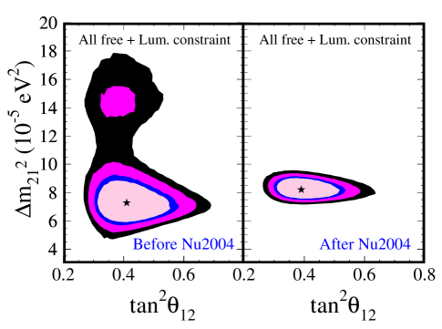
Figure 2: ‘Before’ and ‘After’ oscillation parameters: Solar plus reactor measurements. The figure shows the 90%, 95%, 99%, and 3$\sigma$ allowed regions for oscillation parameters that are obtained by a global fit of the available solar [8, 3, 4, 10, 13, 14, 5, 12] and reactor data [1, 6, 7]. Left (Right) panel corresponds to analysis of data available before (after) Neutrino 2004 conference. The ‘after’ panels contain data from either ref. [1] (new KamLAND data) or ref. [2] (new gallium data).

Figure 2 compares the allowed regions of solar neutrino oscillation parameters that were permitted before Neutrino 2004 with the allowed regions that are permitted after Neutrino 2004. The upper ($\sim 1.4\times 10^{-4}\,{\rm eV^{2}}$) allowed region and the connecting region between the upper and lower ($\sim 7\times 10^{-5}\,{\rm eV^{2}}$) allowed regions, all of which is permitted by the data existing before Neutrino 2004, is disfavored at more than $3\sigma$ after the data presented at Neutrino 2004 are included. The elimination of the higher $\Delta m^{2}_{21}$ regions is due to the greater precision of the new KamLAND data [1].

Maximal mixing is strongly excluded both before and after Neutrino 2004,

$$\tan^{2}\theta_{12}<1.0~{}{\rm at}~{}5.5\sigma(5.8\sigma)~{}~{}~{}~{}{\rm Before~{}(After)}.$$ (7)

5.2 Sterile neutrinos

We consider in this subsection the constraints on the admixture of sterile neutrinos. We concentrate on scenarios in which all $\Delta m^{2}$’s but one are large enough to be averaged out in the solar and reactor neutrino experimental setups [22] . The 4-$\nu$ models invoked to explain the LSND signal [46] together with the solar and atmospheric neutrino data are an example of the kind of model we consider here.

There are strong constraints of $\nu_{e}$ admixtures with large $\Delta m^{2}$’s from the lack of observation of oscillations of reactor $\overline{\nu}_{e}$ at short distances [7, 47, 48]. These constraints imply that in the scenarios considered here solar and reactor oscillations can be understood as a single wavelength oscillation of $\nu_{e}$ into a state that is a linear combination of active ($\nu_{a}$) and sterile ($\nu_{s}$) neutrino states, $\nu_{e}\to\cos\eta\,\nu_{a}\,+\,\sin\eta\,\nu_{s}$ where $\eta$ is the parameter that describes the active-sterile admixture. The sterile contribution to the solar neutrino fluxes can also be parameterized in terms of $\sin^{2}\eta$ or, alternatively, in terms of a derived parameter $f_{\rm B,\,sterile}$, the sterile fraction of the ⁸B neutrino flux (see discussion in ref [23]).

The $1(3)\sigma$ allowed range for the active-sterile admixture is

$$\sin^{2}\eta\leq 0.09(0.35)~{}{\rm at}~{}1(3)\sigma$$ (8)

for our global analysis of the existing solar plus reactor data. The fundamental parameter describing the sterile fraction is $\sin^{2}\eta$ (see ref [23]). However, it is convenient to think in terms of a sterile fraction of the flux, $f_{\rm B,\,sterile}$ , which is potentially observable in the Super-Kamiokande and SNO experiments. This range corresponds to

$$f_{\rm B,\,sterile}~{}=~{}0.0^{+0.06}_{-0.00}(^{+0.25}_{-0.00})~{}~{}({\rm solar+reactor})\,.$$ (9)

The limits on sterile neutrinos are not changed significantly by the additional data released at Neutrino 2004 (see the last column of Table 2).

5.3 Solar neutrino fluxes

Table 3 presents the best-fit solar neutrino fluxes and their uncertainties that are obtained from a global fit to all the solar and reactor data. The fluxes are normalized to the predicted fluxes in the standard solar model [31].

The most remarkable fact about table 3 is that the inferred ranges of the solar neutrino fluxes are very robust. The fluxes and their uncertainties are practically unchanged by the data released at Neutrino 2004. The p-p and ⁸B solar neutrino fluxes are determined ($1\sigma$) to 2% and 5%, respectively, and the ⁷Be and the CNO fluxes (see below) are very poorly determined.

Table 3: Solar neutrino fluxes. The table presents the best-fit solar neutrino fluxes normalized to the BP04 solar model fluxes [31]. The 1$\sigma$ (3$\sigma$) uncertainty ranges are determined from all the solar and reactor data available Before (upper row) and After (lower row) the Neutrino 2004 conference. The last entry entry in the table is the fraction of the total solar luminosity that is associated with CNO nuclear fusion reactions. The fit to existing solar neutrino experiments prefers a CNO luminosity that is less than 0.1%, see ref. [24].

Analysis	pp	7Be	8B	${\rm L}_{\rm CNO}$ %
Before Nu2004	$1.02^{+0.02}_{-0.02}$ (${}^{+0.06}_{-0.06}$)	$0.91^{+0.25}_{-0.62}$ (${}^{+0.79}_{-0.91}$)	$0.88^{+0.04}_{-0.04}$ (${}^{+0.11}_{-0.12}$)	$0.0^{+2.8}_{-0.0}$ (${}^{+7.6}_{-0.0}$)
After Nu2004	$1.01^{+0.02}_{-0.02}$ (${}^{+0.06}_{-0.06}$)	$1.03^{+0.24}_{-1.03}$ (${}^{+0.77}_{-1.03}$)	$0.87^{+0.04}_{-0.04}$ (${}^{+0.09}_{-0.11}$)	$0.0^{+2.7}_{-0.0}$ (${}^{+7.3}_{-0.0}$)

All of the estimates of the solar neutrino fluxes and their uncertainties are insensitive to which of the six KamLAND analysis options (see section 3.2) we employ. The best-fit $p-p$ neutrino flux and the $1\sigma$ and $3\sigma$ $p-p$ flux uncertainties are the same for all six options to the numerical accuracy of table 3. The best-fit ⁸B neutrino flux varies by only $0.25\sigma$, the $1\sigma$ uncertainty is the same in all cases, and the $3\sigma$ range varies by 5% for all six options. The range of solutions found for the ⁷Be solar neutrino flux using the six different analysis options is negligible compared to the uncertainties that arise from the experimental data and that are shown in table 3.

The global analysis yields the following values for the CNO fluxes using data available before Neutrino 2004:

$${}^{13}{\rm N}=0.0^{+4.3}_{-0.0};~{}~{}^{15}{\rm O}=0.0^{+2.4}_{-0.0};~{}~{}^{17}{\rm F}=0^{+2.2}_{-0.0}~{}~{}~{}~{}{\rm Before}.$$ (10)

Using all the data available after Neutrino 2004, the CNO fluxes are:

$${}^{13}{\rm N}=0.0^{+4.1}_{-0.0};~{}~{}^{15}{\rm O}=0.0^{+2.3}_{-0.0};~{}~{}^{17}{\rm F}=0^{+2.1}_{-0.0}~{}~{}~{}~{}{\rm After}.$$ (11)

The global fit to all the data yields a best-fit CNO fractional contribution to the solar luminosity that is less than $0.1$%, much less than the range, 0.8% to 1.6%, implied [31] by standard solar model calculations. However, the constraint shown in table  3 is consistent with the BP04 solar model prediction at $1\sigma$.

5.4 How sensitive are the global results to the precise gallium event rate?

Table 4: Analysis of solar and reactor data assuming different values of the event rate in gallium solar neutrino experiments. The table presents results for three different assumed gallium solar neutrino event rates; all the other solar and reactor data available prior to Neutrino 2004 were used unchanged in the analyses. The three cases considered are a low gallium rate (average of GNO and SAGE for the period 1998-2003), the average gallium rate (GALLEX/GNO and SAGE 1991-2003), and a high gallium rate (GALLEX and SAGE 1991-1997). The solar neutrino fluxes are treated as free parameters, constrained by energy conservation (the luminosity constraint), and are normalized to the BP04 predicted fluxes.

Gallium Rate (SNU)	$63.3\pm 3.6$	$68.1\pm 3.75$	$77.8\pm 5.0$
$\Delta m^{2}_{21}(10^{-5}eV^{2})$	$8.2^{+0.3}_{-0.3}$ (${}^{+1.0}_{-0.8}$)	$8.2^{+0.3}_{-0.3}$ (${}^{+1.0}_{-0.8}$)	$8.2^{+0.3}_{-0.3}$ (${}^{+1.0}_{-0.8}$)
$\tan^{2}\theta_{12}$	$0.39^{+0.05}_{-0.04}$ (${}^{+0.19}_{-0.11}$)	$0.39^{+0.05}_{-0.04}$ (${}^{+0.19}_{-0.11}$)	$0.38^{+0.05}_{-0.05}$ (${}^{+0.21}_{-0.11}$)
$p-p$	$1.03^{+0.02}_{-0.02}$ (${}^{+0.05}_{-0.07}$)	$1.01^{+0.02}_{-0.02}$ (${}^{+0.06}_{-0.06}$)	$0.99^{+0.02}_{-0.02}$ (${}^{+0.07}_{-0.06}$)
8B	$0.87^{+0.04}_{-0.04}$(${}^{+0.09}_{-0.11}$)	$0.87^{+0.04}_{-0.04}$(${}^{+0.09}_{-0.11}$)	$0.88^{+0.04}_{-0.04}$(${}^{+0.09}_{-0.12}$)
7Be	$0.25^{+0.85}_{-0.25}$(${}^{+1.37}_{-0.25}$)	$1.03^{+0.24}_{-1.03}$ (${}^{+0.77}_{-1.03}$)	$1.29^{+0.26}_{-0.57}$ (${}^{+0.74}_{-1.29}$)

The average rate of the two gallium experiments, GALLEX/GNO and SAGE, was slightly higher in the earlier period of data taking, 1991-1997, than it was in the later period, 1998-2003 [49, 50]. In the earlier period, the average rate of the two experiments was ($77.8\pm 5.0$) SNU, while in the latter period, the average rate was ($63.3\pm 3.6$) SNU [49]. The grand average for the period in question, 1991-2003, is ($68.1\pm 3.75$) SNU.

V. Gavrin [49] has raised the possibility that the difference between the observed rates in the earlier period and in the latter period could be due to a time-dependence of the lower-energy $p-p$ and ⁷Be fluxes. In this phenomenological interpretation, the hypothesized variation could not be observed in other solar neutrino experiments because of a lack of sensitivity to the $p-p$ or ⁷Be solar neutrinos or because of the long time scale and small amplitude of the assumed time dependence. Only further long-term measurements with low energy solar neutrino detectors can settle experimentally this question. We address here instead a related issue.

We investigate in this subsection the extent to which the precise value of the gallium rate influences the inferred neutrino properties and solar neutrino fluxes that are obtained by a global solution to all the available solar and reactor data.

Table 4 presents the results of three different global analyses corresponding to the three different assumed gallium event rates: ($77.8\pm 5.0$) SNU (1991-1997), ($68.1\pm 3.75$) SNU (1991-2003), and ($63.3\pm 3.6$) SNU (1998-2003). All the other solar neutrino and reactor anti-neutrino data available prior to Neutrino 2004 were used unchanged in the analyses, which were performed as described in section 4.2.

The results obtained from the global analyses are remarkably robust with respect to the assumed gallium event rate. Within the range considered from 63 SNU to 78 SNU, the inferred values for $\Delta m^{2}_{21}$ and $\tan^{2}\theta_{12}$ are essentially the same for all three choices of the gallium rate. The three best-constrained solar neutrino fluxes, $p-p$, ⁸B, and ⁷Be, also change very little (changes less than $1\sigma$)as the gallium rate is varied within the allowed range.

6 Predicted rates for ⁷Be, $p-p$, and $pep$ experiments

In this section, we summarize the predicted rates for future $\nu-e$ scattering experiments with ⁷Be, $p-p$, and $pep$ solar neutrinos.

Whether or not the ⁷Be solar neutrino flux is treated as a free parameter affects strongly the uncertainty, and the best estimate, of the predicted rate in a ⁷Be $\nu-e$ scattering experiment. If we perform the global analysis of solar plus reactor experiments assuming that the BP004 calculations for the solar neutrino fluxes and their uncertainties are valid then the predicted rate in a ⁷Be $\nu-e$ scattering experiment [51] is, with $1\sigma$ ($3\sigma$) uncertainties:

$$\left[{\rm{}^{7}Be}\right]_{\rm\nu-e}~{}=~{}0.665\pm 0.015\,(^{+0.045}_{-0.040})\,\,[{\rm BP04~{}prediction}].$$ (12)

Here $\left[{\rm{}^{7}Be}\right]_{\rm\nu-e}$ is the $\nu-e$ scattering rate in units of the rate that would be expected if the BP04 solar model were exactly correct and neutrinos did not oscillate. Thus, if we use the solar model calculation of the ⁷Be neutrino flux and its uncertainty, then the predicted event rate for the ⁷Be rate experiment has a precision of $\pm 3$%. If instead we treat all of the neutrino fluxes as free parameters, then the uncertainties are much larger:

$$\left[{\rm{}^{7}Be}\right]_{\rm\nu-e}~{}=~{}0.63^{+0.13}_{-0.24}(^{+0.44}_{-0.57})\,\,{\rm[all~{}fluxes~{}free+luminosity~{}constraint]}\,.$$ (13)

The result for $\nu-e$ scattering that is given in eq. (12) and eq. (13) includes neutrinos from all the solar neutrino fluxes that produce recoil electrons with energies in the range 0.25-0.8 MeV. Most of the recoil electrons in the selected energy range are produced by ⁷Be neutrinos, although there are small contributions from CNO, $pep$, and $p-p$ neutrinos (whose fluxes we estimate by taking the values from the BP04 solar model [31]). The best-estimates given in eq. (12) and eq. (13) would be changed by much less than $1\sigma$, to 0.664 and 0.68, respectively, if we included only events caused by ⁷Be neutrinos.

The predictions given in eq. (12) and eq. (13) are robust. The results obtained here are well within the $1\sigma$ quoted uncertainties of the pre-Neutrino 2004 predictions (see ref. [25]).

The corresponding predicted rates in a $p-p$ $\nu-e$ scattering experiment are, with $1\sigma$ ($3\sigma$) uncertainties:

$$\left[{\rm p-p}\right]_{\rm\nu-e}~{}=~{}0.707^{+0.011}_{-0.013}(^{+0.041}_{-0.039})\,[{\rm BP04~{}prediction}]\,,$$ (14)

and

$$\left[{p-p}\right]_{\rm\nu-e}~{}=~{}0.716^{+0.014}_{-0.016}(^{+0.050}_{-0.044})\,{\rm[all~{}fluxes~{}free+luminosity~{}constraint]}\,.$$ (15)

The predicted rates in a $pep$ $\nu-e$ scattering experiment are:

$$\left[{\rm pep}\right]_{\rm\nu-e}~{}=~{}0.644^{+0.011}_{-0.013}(^{+0.045}_{-0.037})\,[{\rm BP04~{}prediction}]\,,$$ (16)

and

$$\left[{pep}\right]_{\rm\nu-e}~{}=~{}0.652^{+0.015}_{-0.016}(^{+0.053}_{-0.041})\,{\rm[all~{}fluxes~{}free+luminosity~{}constraint]}\,.$$ (17)

The predicted rates of the $p-p$ and $pep$ solar neutrino scattering experiments are robust [25]. The $p-p$ and $pep$ rates are affected by less than $1\sigma$ by the choice of whether or not we use flux predictions from the BP04 solar model or allow the fluxes to vary as free parameters.

Since the $p-p$, $pep$, and ⁷Be solar neutrinos sample the survival probability at different energies (as reflected by the different values given in the predicted rates shown above), it is important to measure $\nu-e$ scattering rates for all three fluxes.

7 CPT bound

In this section, we compare the regions of allowed oscillation parameters for neutrinos and anti-neutrinos in order to constrain the violation of CPT in the neutrino sector [52, 53, 54, 55, 19, 56]. Our discussion follows the pre-KamLAND analysis of ref. [19], in which expected results from KamLAND were simulated.

Figure 1 shows, in the left-hand panel, the 90%, 95%, 99%, and 3$\sigma$ allowed regions for oscillation parameters that are obtained by a global solution to all the available solar data and, in the right-hand panel, to all the available reactor data. The juxtaposition of purely solar and purely reactor data in the same figure allows a visual comparison of the constraints on neutrino and on anti-neutrino oscillation parameters. The allowed regions obtained by a global solution to all the available solar and reactor data are shown in figure 2.

We characterize, following ref. [19], the sensitivity of reactor and solar neutrino experiments to CPT violation by the quantity

$$\langle\Delta CPT\rangle~{}=~{}2\frac{|\rm R_{\nu\nu}-R_{\bar{\nu}\bar{\nu}}|}{\left[\rm R_{\nu\nu}+R_{\bar{\nu}\bar{\nu}}\right]}$$ (18)

Here both ${\rm R_{\nu\nu}}$ and ${\rm R_{\bar{\nu}\bar{\nu}}}$ are computed for the present KamLAND experimental set up, but using, respectively, values for ($\Delta m^{2}_{\nu}$, $\theta_{\nu}$) and for ($\Delta m^{2}_{\bar{\nu}}$, $\theta_{\bar{\nu}}$) within the allowed regions of the solar-only analysis (section 4.1 and the lower left-hand panel of figure 1) and of the KamLAND-only analysis (section 3.1 and the lower right-hand panel of figure 1) at a given CL. Then, $\langle\Delta CPT\rangle$ is the number of events observed in KamLAND minus the number of events that are expected from the solar-only analysis if neutrinos and anti-neutrinos had exactly the same oscillation parameters, divided by the average.

The maximum value of $\langle\Delta CPT\rangle$ is

$$\langle\Delta CPT\rangle~{}\leq~{}0.52~{}(1.01)\ \ \ \ {\rm at}\ \ 1\sigma\ \ (3\sigma).$$ (19)

Matter effects, which simulate CPT violation, contribute less than 0.01 (0.05) to $\langle\Delta CPT\rangle$ for neutrino parameters in the 1$\sigma$ (3$\sigma$) KamLAND-only allowed regions (lower right-hand panel of figure 1) and 0.08 (0.09) for neutrino parameters in the Solar-only allowed regions (lower left-hand panel of figure 1).

This experimental upper limit on $\langle\Delta CPT\rangle$ can be used to test arbitrary future conjectures of CPT violation. Following ref. [19], we consider an effective interaction which has been discussed by Coleman and Glashow [52, 53], and by Colladay and Kostelecky [54], that violates both Lorentz invariance and CPT invariance. The interaction is of the form

$${\mathcal{L}}(\Delta CPT))~{}=~{}\bar{\nu}_{\rm L}^{\alpha}{b^{\alpha\beta}_{\mu}}{\gamma_{\mu}}{\nu_{\rm L}^{\beta}},$$ (20)

where $\alpha,\beta$ are flavor indices, L indicates that the neutrinos are left-handed, and $b$ is a Hermitian matrix. We discuss the special case with rotational invariance in which $b_{0}$ and the mass-squared matrix are diagonalized by the same mixing angle. We also assume that there are only two interacting neutrinos (or anti-neutrinos) and follow previous authors in defining $\eta$ as the difference of the phases in the unitary matrices that diagonalize $\Delta m^{2}$ and the CPT odd quantity $\delta b$, which is the difference between the two eigenvalues of $b_{0}$.

When the relative phase is $\eta=0$, the survival probabilities of neutrino and anti-neutrinos take on an especially simple form. In the case of reactor antineutrinos, the oscillations occur in vacuum to an excellent approximation (matter effects are negligible in the range of parameters allowed by KamLAND data, see details in ref. [23]):

$$P_{\rm ee}~{}=~{}\cos^{4}\theta_{13}~{}\left[1-\sin^{2}2\theta_{12}\sin^{2}\left(\frac{\Delta m^{2}_{21}L}{4E_{\nu}}-\frac{\delta bL}{2}\right)\right].$$ (21)

In the case of solar neutrinos, sensitivity to $\delta b$ in the oscillation phase is lost because of the fast oscillations due to the $\Delta m^{2}_{21}$ term. In both cases, solar and reactor neutrinos, the mixing in vacuum is unchanged. The standard survival probability and mixing in matter are valid with a modified ratio of matter to vacuum effects given by

$$\beta~{}=~{}\frac{2\sqrt{2}G_{F}\cos^{2}\theta_{13}n_{e}E_{\nu}}{\Delta m^{2}_{21}+2\,\delta b\,E_{\nu}}\,.$$ (22)

We have reanalyzed solar and reactor neutrino data with the modified probabilities that contain an extra free parameter $\delta b$. We obtain the $\chi^{2}$ distribution on $\delta b$ by marginalizing over all other variables. The resulting upper bound on the violation of CPT invariance is:

$$\delta b<0.6\,(1.5)\times 10^{-20}\,{\rm GeV},~{}~{}\eta=0\ \ \ \ {\rm at}\ \ 1\sigma\,(3\sigma).$$ (23)

8 Summary and discussion

We summarize and discuss in this section our main conclusions.

The most important feature of the recent KamLAND results [1] is the detection of the spectral energy distortion that was expected for oscillations with parameters within the Large Mixing Angle region. The distortion implies that the $3\sigma$ region from the KamLAND-only analysis no longer extends to masses larger than $\Delta m^{2}_{21}=2\times 10^{-4}$ eV².

Comparing the upper and lower right hand (KamLAND-only) panels of figure 1, one can see clearly the effect of the observed spectral distortion in eliminating previously allowed regions with a large $\Delta m^{2}_{21}$. In the now-excluded large mass regions, the predicted spectral distortions are too small to fit the KamLAND data.

As a consequence of the observation of spectral distortion, the largest change in the globally allowed regions of neutrino parameters is the elimination of the larger $\Delta m^{2}_{21}$ regions in the global solution. This constriction of the globally allowed regions can be seen visually by comparing the left and right hand panels of figure 2. The large $\Delta m^{2}_{21}$ regions were previously allowed in the global solution at 99% CL.

The globally allowed range of $\Delta m^{2}_{21}$ is reduced by a factor of 1.7 (5) at $1\sigma(3\sigma)$ compared to the previously allowed range (see figure 2 and table 2). The best-fit value of $\Delta m^{2}_{21}$ is increased by about 15% by the new data released at Neutrino 2004, which represents a 1.4$\sigma$ shift from the previous global minimum in the before Neutrino 2004 analysis.

The allowed ranges, as well as the best-fit values, of $\tan^{2}\theta_{12}$ and $\sin^{2}\theta_{13}$ are, as is shown in table 2, not affected significantly by the new data release. For example, the best-fit value of $\tan^{2}\theta_{12}$ is changed by only $0.4\sigma$ and the $1\sigma$ range of uncertainty is decreased by 10%. For $\sin^{2}\theta_{13}$, the $3\sigma$ bound is decreased by 10%.

The amount by which maximal mixing ($\tan\theta_{12}=1$)is disfavored is $5.4\sigma$ from just solar neutrino measurements (before and after Neutrino 2004) and $5.8\sigma$ from a global solution of all the solar and reactor data available after Neutrino 2004.

The upper limit to the parameter $\sin^{2}\eta$ that characterizes sterile neutrinos is very little affected by the recent data release, as is also shown table 2. Allowing all of the neutrino fluxes to be free parameters, the present upper bound on $\sin^{2}\eta$ is equivalent to a maximum sterile fraction of 6% for the ⁸B solar neutrino flux (see section 5.2).

We conclude that the parameters which describe solar neutrino oscillations are robustly determined, if not yet as precise as we would like. This is the first major result of the present reanalysis.

Our second major result is that the allowed ranges of the $p-p$ and ⁸B solar neutrino fluxes are robustly determined by the existing solar neutrino and reactor data.

Table 3 shows that both the best-fit values and the $1\sigma$ and $3\sigma$ allowed ranges of all three of the major solar neutrino fluxes, the $p-p$, ⁷Be, and ⁸B neutrinos, are essentially unaffected by the data released at Neutrino 2004. The $\pm 2$ % precision with which the $p-p$ neutrino flux is determined is due to the luminosity constraint as well as the neutrino measurements.

The ⁷Be and CNO neutrino fluxes are very poorly determined (both Before and After Neutrino 2004)(see table 3 and eq. (11)). The upper limit to the fraction of the solar luminosity that is associated with CNO fusion reactions remains about a factor of six above the value predicted by the BP04 solar model (see also table 3).

The rate of a ⁷Be neutrino-electron scattering experiment is rather well predicted if the BP04 solar model calculations of the solar neutrino fluxes are assumed and is rather poorly predicted if all the solar neutrino fluxes are allowed to be free parameters in fitting the existing solar and reactor data. If the solar model predictions are adopted, then the predicted rate is $0.665\pm 0.015\,(^{+0.045}_{-0.040})$ of the rate implied by the BP04 solar model in the absence of neutrino oscillations. The rate predicted if the neutrino fluxes are treated as free parameters is $0.63^{+0.13}_{-0.24}(^{+0.44}_{-0.57})$ of the solar model prediction without oscillations.

The predicted rates for $p-p$ and $pep$ solar neutrino experiments are robust and essentially independent of whether one uses fluxes from the BP04 solar model or allows the fluxes to vary freely subject to the luminosity constraint. If we use the BP04 fluxes, the predicted rate of a $p-p$ experiment is $\left[{\rm p-p}\right]_{\rm\nu-e}~{}=~{}0.707^{+0.011}_{-0.013}(^{+0.041}_{-0.039})$ and the predicted rate for a $pep$ experiment is $\left[{\rm pep}\right]_{\rm\nu-e}~{}=~{}0.644^{+0.011}_{-0.013}(^{+0.045}_{-0.037})$.

Since the ⁷Be, $p-p$, and $pep$ fluxes sample the survival probability curve at different energies (see the results and discussion in section 6), it is important to measure the $\nu-e$ scattering of all three of these fluxes. According to equation (8) and figure 1 of Ref. [25], all three of these fluxes should be in the region of neutrino oscillation space in which vacuum neutrino oscillations dominate over matter oscillations.

CPT violation in the neutrino sector is limited by the comparison of the allowed neutrino oscillation regions (left hand panels of figure 1) with the allowed anti-neutrino oscillation regions (right hand panels of figure 1). This comparison leads to an accurate experimental limit. This limit is presented in both a model independent and a model dependent way in section 7.

We have verified that our results are insensitive (changes much less than $1\sigma$) to which of six approaches we use in analyzing the KamLAND data (section 3.2), which of the published ⁸B neutrino energy spectra we adopt (section 4.2.2), and the precise value of the gallium solar neutrino event rate (section 5.4).

Appendix A Analysis details regarding $\theta_{13}$

Table 2 presents our limit on $\theta_{13}$. In this section, we describe some of the details of the method used to obtain this limit. We shall see that the $\theta_{13}$ bound from the atmospheric and CHOOZ data implies that three neutrino effects are small for solar and reactor experiments. However these three neutrino effects are not totally negligible and they contribute to the final bound on $\theta_{13}$.

The minimum joint description of atmospheric, K2K, solar, and reactor data requires that all the three known neutrinos take part in the oscillation process. The mixing parameters are encoded in the $3\times 3$ lepton mixing matrix which can be conveniently parameterized in the standard form:

$$U=\left(\begin{array}[]{ccc}1&0&0\\ 0&{c_{23}}&{s_{23}}\\ 0&-{s_{23}}&{c_{23}}\end{array}\right)\times\left(\begin{array}[]{ccc}{c_{13}}&0&{s_{13}}e^{i{\delta}}\\ 0&1&0\\ -{s_{13}}e^{-i{\delta}}&0&{c_{13}}\end{array}\right)\times\left(\begin{array}[]{ccc}c_{21}&{s_{12}}&0\\ -{s_{12}}&{c_{12}}&0\\ 0&0&1\end{array}\right)$$ (24)

where $c_{ij}\equiv\cos\theta_{ij}$ and $s_{ij}\equiv\sin\theta_{ij}$. Note that the two Majorana phases are not included in the expression above since they do not affect neutrino oscillations. The angles $\theta_{ij}$ can be taken without loss of generality to lie in the first quadrant, $\theta_{ij}\in[0,\pi/2]$.

We know from the analysis of solar and atmospheric oscillations that the mass differences satisfy:

$$\Delta m^{2}_{\odot}=\Delta m^{2}_{21}\ll|\Delta m_{31}^{2}|=\Delta m^{2}_{\rm atm}.$$ (25)

Under this condition, the joint three-neutrino analysis simplifies. For the solar and KamLAND experiments, the oscillations with the atmospheric oscillation length are completely averaged out and the survival probability takes the form:

$$P^{3\nu}_{ee}=\sin^{4}\theta_{13}+\cos^{4}\theta_{13}P^{2\nu}_{ee}\,,$$ (26)

where in the Sun $P^{2\nu}_{ee}$ is obtained with the modified density $N_{e}\rightarrow\cos^{2}\theta_{13}N_{e}$. The analysis of solar data constrains three of the seven parameters: $\Delta m^{2}_{21},\theta_{12}$ and $\theta_{13}$.

For atmospheric and K2K neutrinos, the solar wavelength is too long to be relevant and the corresponding oscillating phase is negligible. As a consequence, the atmospheric data analysis restricts $\Delta m^{2}_{31}\simeq\Delta m^{2}_{32}$, $\theta_{23}$, and $\theta_{13}$. The mixing angle $\theta_{13}$ is the only parameter common to both solar and atmospheric neutrino oscillations; it potentially allows for some mutual influence. The effect of $\theta_{13}$ is to add a $\nu_{\mu}\rightarrow\nu_{e}$ contribution to the atmospheric oscillations. Finally, for the CHOOZ experiment, the solar wavelength is unobservable if $\Delta m^{2}_{21}\leq 8\times 10^{-4}~{}{\rm eV}^{2}$. The relevant survival probability oscillates with a wavelength determined by $\Delta m^{2}_{31}$ and an amplitude determined by $\theta_{13}$.

The above considerations imply that the global analysis factorizes as

$$\chi^{2}_{\rm global}=\chi^{2}_{\rm solar+Kamland}(\Delta m^{2}_{21},\theta_{12},\theta_{13})+\chi^{2}_{\rm atm+K2K+CHOOZ}(\Delta m^{2}_{31},\theta_{23},\theta_{13})\,.$$ (27)

Thus the 3-$\nu$ oscillation effects in the analysis of solar and KamLAND data are obtained from the study of:

$$\chi^{2}_{global}|_{\rm marg}(\Delta m^{2}_{21},\theta_{12},\theta_{31})=\chi^{2}_{\rm solar+Kamland}(\Delta m^{2}_{21},\theta_{12},\theta_{13})+\chi^{2}_{\rm atm+K2K+CHOOZ}|_{\rm marg}(\theta_{13})\,.$$ (28)

We denote by $\chi^{2}_{\rm atm+K2K+CHOOZ}|_{\rm marg}$ the $\chi^{2}$ analysis of atmospheric, K2K and CHOOZ data after marginalization over $\Delta m^{2}_{31}$ and $\theta_{23}$.

The present strong bound on $\theta_{13}$ is mostly determined by $\chi^{2}_{\rm atm+K2K+CHOOZ}|_{marg}(\theta_{13})$ and arises from the non-observation of $\overline{\nu}_{e}$ oscillations at CHOOZ with an atmospheric wavelength. Here we have used the results from our updated three-neutrino oscillation analysis [36] of atmospheric [57], K2K [29], and CHOOZ [7] data which we briefly summarize.

The basic techniques employed can be found in ref. [35], but we have updated the atmospheric neutrino analysis to include the results from the final Super-Kamiokande phase I analysis [57]. In particular we make use of the new three-dimensional fluxes from Honda [58] as well as the improved interaction cross sections which agree better with the measurements performed with near detector in K2K. We have also improved our statistical analysis of the atmospheric data (see ref. [37] for details).

As a result of the inclusion of all of these effects, the allowed region for $\Delta m^{2}_{31}$ is shifted to lower values and the 3$\sigma$ bound on $\theta_{13}$ from $\chi^{2}_{\rm atm+K2K+CHOOZ}|_{marg}(\theta_{13})$ weakened slightly (from $\sin^{2}\theta_{13}\leq 0.056$ to 0.059). Also the best-fit value of $\sin^{2}\theta_{13}$ is not exactly at $\sin^{2}\theta_{13}=0$ but rather at $\sin^{2}\theta_{13}=0.006$ (although $\sin^{2}\theta_{13}$ differs from 0.0 only by $0.5\sigma$). This fact that $\sin^{2}\theta_{13}$ is not exactly zero is due to the atmospheric neutrino data, in particular to the slight excess of sub-GeV e-like events which are better described with a non-vanishing value of $\theta_{13}$.

The inclusion of the KamLAND and solar data further strengthens the $\theta_{13}$ bound as is reflected in Table 2. Before the new KamLAND and solar results, the $1\sigma$ ($3\sigma$) bound on $\theta_{13}$ from the global 3–$\nu$ analysis was $\sin^{2}\theta_{13}<0.019(0.054)$. This bound is now improved by about 10% to $\sin^{2}\theta_{13}<0.016(0.048)$.

References

- [1] KamLAND collaboration, Measurement of neutrino oscillations with KamLAND: Evidence of spectral distortion, hep-ex/040621.
- [2] C. Cattadori, Results from radiochemical solar neutrino experiments, talk at XXIst International Conference on Neutrino Physics and Astrophysics (NU2004), Paris, June 14–19, 2004.
- [3] V. Gavrin, Results from the Russian American gallium experiment (SAGE), talk at VIIIth International Conference on Topics in Astroparticle and Underground Physcis (TAUP03), Seattle, Sept. 5–9, 2003; SAGE collaboration, J.N. Abdurashitov et al., Measurement of the solar neutrino capture rate by the Russian-American gallium solar neutrino experiment during one half of the 22-year cycle of solar activity, J. Exp. Theor. Phys. 95 (2002) 181 [astro-ph/0204245].
- [4] GALLEX collaboration, W. Hampel et al., GALLEX solar neutrino observations: results for GALLEX IV, Phys. Lett. B 447 (1999) 127.
- [5] E. Bellotti, The Gallium Neutrino Observatory (GNO), talk at VIIIth International Conference on Topics in Astroparticle and Underground Physcis (TAUP03), Seattle, Sept. 5–9, 2003 ; GNO collaboration, M. Altmann et al., GNO solar neutrino observations: results for GNO I, Phys. Lett. B 490 (2000) 16.
- [6] KamLAND collaboration, K. Eguchi et al., First results from KamLAND: evidence for reactor anti-neutrino disappearance, Phys. Rev. Lett. 90 (2003) 021802 [hep-ex/0212021].
- [7] M. Apollonio et al., Limits on neutrino oscillations from the CHOOZ experiment, Phys. Lett. B 466 (1999) 415.
- [8] B.T. Cleveland et al., Measurement of the solar electron neutrino flux with the Homestake chlorine detector, Astrophys. J. 496 (1998) 505.
- [9] Y. Fukuda et al., Solar neutrino data covering solar cycle 22, Phys. Rev. Lett. 77 (1996) 1683.
- [10] Super-Kamiokande Collaboration, S. Fukuda et al., Solar and hep neutrino measurements from 1258 days of Super-Kamiokande data, Phys. Rev. Lett. 86 (2001) 5651.
- [11] SNO Collaboration, Q.R. Ahmad et al., Measurement of the Rate of Interactions produced by Solar Neutrinos at the Sudbury Neutrino Observatory, Phys. Rev. Lett. 87 (2001) 071301.
- [12] SNO Collaboration, S.N. Ahmed et al., Measurement of the total active solar neutrino flux at the Sudbury Neutrino Observatory with enhanced neutral current sensitivity, Phys. Rev. Lett. 92 (2004), 181301 [nucl-ex/0309004].
- [13] SNO collaboration, Q.R. Ahmad et al., Direct evidence for neutrino flavor transformation from neutral-current interactions in the Sudbury Neutrino Observatory, Phys. Rev. Lett. 89 (2002) 011301 [nucl-ex/0204008].
- [14] SNO collaboration, Q.R. Ahmad et al., Measurement of day and night neutrino energy spectra at SNO and constraints on neutrino mixing parameters, Phys. Rev. Lett. 89 (2002) 011302 [nucl-ex/0204009].
- [15] A. Friedland, C. Lunardini and C. Peña-Garay, hep-ph/0402266.
- [16] M. M. Guzzo, P. C. de Holanda and O. L. G. Peres, Effects of non-standard neutrino interactions on MSW-LMA solution, Phys. Lett. B 591, 1 (2004); O. G. Miranda, M. A. Tortola, J. W. F. Valle, Are solar neutrino oscillations robust?, arXiv:hep-ph/0406280.
- [17] P.C. de Holanda and A.Y. Smirnov, Searches for sterile component with solar neutrinos and KamLAND, hep-ph/0211264.
- [18] V. Berezinsky, M. Narayan and F. Vissani, Mirror model for sterile neutrinos, Nucl. Phys. B 658 (2003) 254.
- [19] J.N. Bahcall, V. Barger and D. Marfatia, How accurately can one test CPT conservation with reactor and solar neutrino experiments?, Phys. Lett. B 534 (2002) 120.
- [20] V.N. Gribov and B.M. Pontecorvo Phys. Lett. B 28 (1969) 493
- [21] L. Wolfenstein, Neutrino oscillations in matter, Phys. Rev. D 17 (1978) 2369; S.P. Mikheyev and A.Y. Smirnov, Resonance enhancement of oscillations in matter and solar neutrino spectroscopy, Sov. Jour. Nucl. Phys. 42 (1985) 913.
- [22] D. Dooling, C. Giunti, K. Kang and C.W. Kim, Matter effects in four-neutrino mixing, Phys. Rev. D 61 (2000) 073011; C. Giunti, M.C. Gonzalez-Garcia and C. Peña-Garay, Four-neutrino oscillation solutions of the solar neutrino problem, Phys. Rev. D 62 (2000) 013005.
- [23] J.N. Bahcall, M.C. Gonzalez-Garcia and C. Peña-Garay, Solar neutrinos before and after KamLAND, J. High Energy Phys. 02 (2003) 009 [hep-ph/0212147].
- [24] J.N. Bahcall, M.C. Gonzalez-Garcia and C. Peña-Garay, Does the sun shine by pp or CNO fusion reactions?, Phys. Rev. Lett. 90 (2003) 131301.
- [25] J.N. Bahcall and C. Peña-Garay, Global analyses as a road map to solar neutrino fluxes and oscillation parameters, J. High Energy Phys. 11 (2003) 004.
- [26] G.L. Fogli, E. Lisi, A. Marrone and A. Palazzo, Evidence for Mikheyev-Smirnov-Wolfenstein effects in solar neutrino flavor transitions, Phys. Lett. B 583 (2004) 149 [arXiv:hep-ph/0309100]; M. Maltoni, T. Schwetz, M.A. Tortola and J.W. Valle, Status of three-neutrino oscillations after the SNO-salt data, Phys. Rev. D 68 (2003) 113010 [arXiv:hep-ph/0309130]; P.C. de Holanda and A.Y. Smirnov, Solar neutrinos: the SNO salt phase results and physics of conversion, Astropart. Phys. 21 (2004) 287 [arXiv:hep-ph/0309299]; P. Aliani, V. Antonelli, M. Picariello and E. Torrente-Lujan, The neutrino mass matrix after Kamland and SNO salt enhanced results, arXiv:hep-ph/0309156; P. Aliani, V. Antonelli, R. Ferrari, M. Picariello and E. Torrente-Lujan, Analysis of neutrino oscillation data with the recent KamLAND results, arXiv:hep-ph/0406182; A.B. Balantekin and H. Yuksel, Constraints on neutrino parameters from neutral-current solar neutrino measurements, Phys. Rev. D 68 (2003) 113002 [arXiv:hep-ph/0309079]; A. Bandyopadhyay, S. Choubey, S. Goswami, S.T. Petcov and D.P. Roy, Constraints on neutrino oscillation parameters from the SNO salt phase data, Phys. Lett. B 583 (2004) 134 [arXiv:hep-ph/0309174]; P. Creminelli, G. Signorelli and A. Strumia, Frequentist analyses of solar neutrino data, J. High Energy Phys. 05 (2001) 052 [hep-ph/0102234]; A.B. Balantekin, V. Barger, D. Marfatia, S. Pakvasa and H. Yuksel, Physics from future SNO and KamLAND data, arXiv:hep-ph/0405019.
- [27] J.N. Bahcall, The luminosity constraint on solar neutrino fluxes, Phys. Rev. C 65 (2002) 025801.
- [28] M. Spiro and D. Vignaud, Solar model independent neutrino oscillation signals in the forthcoming solar neutrino experiments?, Phys. Lett. B 242 (1990) 279.
- [29] K2K Collaboration, M.H. Ahn et al., Indications of neutrino oscillation in a 250-km long-baseline experiment, Phys. Rev. Lett. 90 (2003) 041801.
- [30] Kamiokande Collaboration, Y. Fukuda et al., Atmospheric muon-neutrino/electron-neutrino ratio in the multiGeV energy range, Phys. Lett. B 335 (1994) 237; R. Becker-Szendy et al., Neutrino measurements with the IMB detector, Nucl. Phys. (Proc. Suppl.) B 38 (1995) 331; Soudan-2 Collaboration, W.W. Allison et al., The atmospheric neutrino flavor ratio from a 3.9 fiducial kiloton-year exposure of Soudan 2, Phys. Lett. B 449 (1999) 137; Super-Kamiokande Collaboration, Y. Fukuda et al., Evidence for oscillation of atmospheric neutrinos, Phys. Rev. Lett. 81 (1998) 1562; M. Shiozawa, Super-Kamiokande, talk at the XXth International Conference on Neutrino Physics and Astrophysics (NU2002), Munich, May 25–30, 2002; MACRO Collaboration, M. Ambrosio et al., Status report of the MACRO experiment for the year 2001, hep-ex/0206027.
- [31] J.N. Bahcall and M.H. Pinsonneault, What do we (not) know theoretically about solar neutrino fluxes?, Phys. Rev. Lett. 92 (2004) 121301 [astro-ph/0402114]
- [32] S.L. Glashow, Partial symmetries of weak interactions, Nucl. Phys. 22 (1961) 579; S. Weinberg, A model of leptons, Phys. Rev. Lett. 19 (1967) 1264; A. Salam, in Elementary Particle Theory, ed. N. Svartholm (Almquist and Wiksells, Stockolm, 1969), p. 367.
- [33] J.N. Bahcall, M.C. Gonzalez-Garcia and C. Peña-Garay, Before and after: how has the SNO neutral current measurement changed things?, J. High Energy Phys. 07 (2002) 054.
- [34] J.N. Bahcall, M.C. Gonzalez-Garcia and C. Peña-Garay, Robust signatures of solar neutrino oscillation solutions, J. High Energy Phys. 04 (2002) 007.
- [35] M.C. Gonzalez-Garcia and C. Peña-Garay, Three-neutrino mixing after the first results from K2K and KamLAND, Phys. Rev. D 68 (2003) 093003 [hep-ph/0306001].
- [36] M.C. Gonzalez-Garcia and M. Maltoni Status of Global Analysis of Neutrino Oscillation Data, arXiv:hep-ph/0404056
- [37] M.C. Gonzalez-Garcia and M. Maltoni, Atmospheric neutrino oscillations and new physics, arXiv:hep-ph/0404085.
- [38] H. Murayama and A. Pierce, Energy spectra of reactor neutrinos at KamLAND, Phys. Rev. D 65 (2002) 013012 [arXiv:hep-ph/0012075].
- [39] T. Schwetz, Variations on KamLAND: Likelihood analysis and frequentist confidence regions, Phys. Lett. B 577, 120 (2003) [arXiv:hep-ph/0308003].
- [40] J.N. Bahcall, M.H. Pinsonneault and S. Basu, Solar models: current epoch and time dependences, neutrinos, and helioseismological properties, Astrophys. J. 555 (2001) 990.
- [41] J.N. Bahcall, M.H. Pinsonneault, S. Basu and J. Christensen-Dalsgaard, Are standard solar models reliable?, Phys. Rev. Lett. 78 (1997) 171 [astro-ph/9610250].
- [42] J.N. Bahcall, E. Lisi, D.E. Alburger, L. De Braeckeleer, S.J. Freedman and J. Napolitano, Standard neutrino spectrum from B decay, Phys. Rev. C 54 (1996) 411.
- [43] J.N. Bahcall, Gallium solar neutrino experiments: absorption cross sections, neutrino spectra, and predicted event rates, Phys. Rev. C 56 (1997) 3391.
- [44] C. E. Ortiz, A. Garcia, R. A. Waltz, M. Bhattacharya and A. K. Komives, Shape of the alpha and neutrino spectra, Phys. Rev. Lett. 85 (2000) 2909.
- [45] W. T. Winter, S. J. Freedman, K. E. Rehm and J. P. Schiffer, The B-8 neutrino spectrum, arXiv:nucl-ex/0406019.
- [46] A. Aguilar et al. [LSND Collaboration], Evidence for neutrino oscillations from the observation of anti-nu/e appearance in a anti-nu/mu beam, Phys. Rev. D 64 (2001), 112007 [arXiv:hep-ex/0104049].
- [47] Y. Declais et al., Search for neutrino oscillations at 15-meters, 40-meters, and 95-meters from a nuclear power reactor at Bugey, Nucl. Phys. B 434 (1995) 503.
- [48] F. Boehm et al., Results from the Palo Verde neutrino oscillation experiment, Phys. Rev. D 62 (2000) 072002.
- [49] V. Gavrin, April 22, 2004, private communication.
- [50] A. Strumia, C. Cattadori, N. Ferrari and F. Vissani, Which solar neutrino data favour the LMA solution?, Phys. Lett. B 541 (2002) 327 [arXiv:hep-ph/0205261].
- [51] BOREXINO collaboration, G. Alimonti et al., Science and technology of BOREXINO: a real time detector for low energy solar neutrinos, Astropart. Phys. 16 (2002) 205.
- [52] S.R. Coleman and S.L. Glashow, Cosmic ray and neutrino tests of special relativity, Phys. Lett. B 405 (1997) 249.
- [53] S.R. Coleman and S.L. Glashow, High-energy tests of Lorentz invariance, Phys. Rev. D 59 (1999) 116008.
- [54] D. Colladay and V.A. Kostelecky, CPT violation and the standard model, Phys. Rev. D 55 (1997) 6760.
- [55] V.D. Barger, S. Pakvasa, T.J. Weiler and K. Whisnant, CPT odd resonances in neutrino oscillations, Phys. Rev. Lett. 85 (2000) 50555.
- [56] H. Murayama, CPT tests: Kaon vs neutrinos, arXiv:hep-ph/0307127.
- [57] A. Habig [Super-Kamiokande Collaboration], Atmospheric neutrino oscillations in SK-I, prepared for the 28th International Cosmic Ray Conferences (ICRC 2003), Tsukuba, Japan, 31 Jul - 7 Aug 2003.
- [58] M. Honda, T. Kajita, K. Kasahara and S. Midorikawa, A new calculation of the atmospheric neutrino flux in a 3-dimensional scheme, arXiv:astro-ph/0404457.