Thermalization of gluons in ultrarelativistic heavy ion collisions by including three-body interactions in a parton cascade

Abstract

We develop a new 3+1 dimensional Monte Carlo cascade solving the kinetic on-shell Boltzmann equations for partons including the inelastic $gg\leftrightarrow ggg$ pQCD processes. The back reaction channel is treated – for the first time – fully consistently within this scheme. An extended stochastic method is used to solve the collision integral. The frame dependence and convergency are studied for a fixed tube with thermal initial conditions. The detailed numerical analysis shows that the stochastic method is fully covariant and that convergency is achieved more efficiently than within a standard geometrical formulation of the collision term, especially for high gluon interaction rates. The cascade is then applied to simulate parton evolution and to investigate thermalization of gluons for a central Au+Au collision at RHIC energy. For this study the initial conditions are assumed to be generated by independent minijets with $p_{T}>p_{0}=2$ GeV. With that choice it is demonstrated that overall kinetic equilibration is driven mainly by the inelastic processes and is achieved on a scale of $1$ fm/c. The further evolution of the expanding gluonic matter in the central region then shows almost an ideal hydrodynamical behavior. In addition, full chemical equilibration of the gluons follows on a longer timescale of about $3$ fm/c.

I Introduction

The main subject of the heavy ion experiments at the Relativistic Heavy Ion Collider (RHIC) at BNL and at the Large Hadron Collider (LHC) at CERN is to create a new state of matter, the Quark Gluon Plasma (QGP), which is expected to be a transient thermal system of interacting quarks and gluons. Due to the confinement free quarks and gluons cannot be detected. The search for QGP has to be carried out by analyzing certain proposed hadronic and electromagnetic signatures [1, 2, 3, 4, 5, 6, 7, 8]. However, the possible signatures of the QGP may also come in part from the late time dynamics of a hadron gas formed after the phase transition [9, 10, 11, 12, 13, 14, 15]. Therefore one needs detailed informations about the creation of the QGP, its lifetime and the hadronization in order to draw reliable conclusions.

Recent measurements [16] at RHIC of the elliptic flow parameter $v_{2}$ for semi-central collisions suggest that - in comparison to fits based on simple ideal hydrodynamical models [17] - the evolving system builds up a sufficiently early pressure and potentially also achieves (local) equilibrium. On the other hand, the system in the reaction is at least initially far from any (quasi-)equilibrium configuration. To address the crucial question of thermalization of gluons and quarks, a number of theoretical analyses have been worked out either using the relaxation time approximation [18, 19, 20, 21] or performing full $3+1$ dimensional Monte Carlo cascade simulations based on the solution of the Boltzmann equations for quarks and gluons [22, 23, 24, 25, 26]. The first parton cascade, VNI, inspired by pQCD including binary elastic scatterings ($2\leftrightarrow 2$) and gluon radiation and fusion ($1\leftrightarrow 2$) was developed by Geiger and Müller [22]. In the simulation for a central Au+Au collision at RHIC energy [27] they concluded that a thermalized QGP will be formed at $\tau\approx 1.8$ fm/c. However, the onset of potential hydrodynamical behavior during the parton evolution was not demonstrated in their analyses. In addition, the treatment of the propagation of off-shell partons in their approach is not clear from a physical point of view. Recently, Molnar and Gyulassy studied the buildup of the elliptic flow at RHIC [28] applying an on-shell parton cascade, MPC [24] (an improved version of ZPC [23]), in which up to now only elastic gluon interactions are included. In their analysis the early pressure can be achieved only if an unrealistic, much higher cross section is being employed. Furthermore, it is known that the elastic (and forward directed) $gg\leftrightarrow gg$ collisions cannot drive the system to kinetic equilibrium, as pointed out in Ref. [29]. This would suggest that the collective flow phenomena observed at RHIC cannot be described via pQCD. On the other hand, the possible importance of the inelastic interactions on overall thermalization was raised in the so-called “bottom up thermalization” picture [30]. It is intuitively clear that gluon multiplication should not only lead to chemical equilibration [31], but also should lead to a faster kinetic equilibration [32, 33]. This represents one (but not all) important motivation for developing a consistent algorithm to handle inelastic processes like $gg\leftrightarrow ggg$.

In solving the transport equations, in most of the cascade models cross sections are interpreted geometrically to model the collision processes. It turns out that in dense matter when the interaction length $\sqrt{\sigma/\pi}$ is not much smaller than the mean free path of particles, causality violation [34, 35] will arise in these cascade models and will lead to numerical artifacts [36, 37]. One way to reduce these artifacts is to apply the common test particle method (or “particle subdivisions”) [38, 39], in which the interaction length of the test particles is reduced by $\sqrt{N_{test}}$, while the mean free path is unchanged. $N_{test}$ denotes the number of the test particles per real particle. However, the limitation of these transport models is obvious: Inelastic collision processes with more than two incoming particles cannot be straightforwardly implemented since it is in general difficult to determine, for instance, a $3\to 2$ process geometrically. Therefore, until now, the role of the inelastic processes in the formation of the QGP has not been studied fully quantitatively.

An alternative collision algorithm suggested in [40, 41, 42] dealt with the transition rate instead of the geometrical interpretation of cross section and determined proceeding collision processes in a stochastic manner by sampling possible transitions in a certain volume and time interval. This collision algorithm opens up the possibility to include the inelastic collision processes into transport simulations solving the Boltzmann equations

$$\left(\frac{\partial}{\partial t}+\frac{{\mathbf{p}}_{1}}{E_{1}}\frac{\partial}{\partial{\mathbf{r}}}\right)\,f_{1}({\mathbf{r}},{\mathbf{p}}_{1},t)={\cal C}_{22}+{\cal C}_{23}+\cdots\,,$$ (1)

where ${\cal C}_{22}$ and ${\cal C}_{23}$ denote the collision term of $2\leftrightarrow 2$ and $2\leftrightarrow 3$ processes. In this paper we will present a newly developed on-shell parton cascade using this sort of stochastic collision algorithm. Also the oftenly employed scheme based on the geometrical interpretation of cross section is discussed and compared with the stochastic algorithm. In particular, we concentrate on the study of the (unphysical) frame dependence. The new transport scheme will then be applied to simulate the parton evolution for a central ultrarelativistic heavy ion collision at highest RHIC energy. The emphasis is put on the investigation of gluon thermalization and their collective dynamics. For this investigation the initial conditions are assumed to be generated by independent minijets [43, 44]. Other initial conditions, like the much discussed “color glass condensate” [45], can also be implemented, but we leave this for a future work. For the present study we consider quarks and gluons as classical Boltzmann particles throughout the paper. The Pauli blocking and gluon enhancement can, in principle, be implemented and will also be discussed elsewhere.

The paper is organized as follows. In Sec. II we consider two-body collision processes and contrast the geometrical with the stochastic collision algorithm. The dynamical evolution of a system within a fixed box is carried out to study global kinetic equilibration. In addition, such calculations are mandatory to debug the operation of the code and to look for the limitation of the algorithms. The implementation of the inelastic collision processes is described in Sec. III. There, we carry out box calculations to study global kinetic and chemical equilibration. In Sec. IV we study thermalization of a parton system in a box with initial conditions sampled according to the production of minijets as expected in a central heavy ion collision at RHIC. The Lorentz or frame (nondependence) and the convergency of results extracted from cascade simulations are investigated in Sec. V. In Sec. VI we then finally present first results of cascade simulations for a central Au+Au collision at RHIC energy. (The readers, who are solely interested in the operation and results of the full $3+1$ dimensional cascade, may directly pass to Sec. VI.) We summarize in Sec. VII and give an outlook for future works. In Appendices A and B more details of the geometrical collision algorithm are given. We list the pQCD partonic scattering cross sections in Appendix C for two-body processes and in Appendix D for $gg\leftrightarrow ggg$ processes. In Appendix E the numerical recipes for Monte Carlo samplings are presented.

II Two-body collision processes

We consider a system consisting of classical, ultrarelativistic particles which are interacting via two-body collisions. The main emphasis is put on the numerical realization of such collision sequences in a relativistic transport simulation, which is theoretically based on the solution of the Boltzmann equations (1) with the following collision term given by

$${\cal C}_{22} = \frac{1}{2E_{1}}\int\frac{d^{3}p_{2}}{(2\pi)^{3}2E_{2}}\,\frac{1}{\nu}\int\frac{d^{3}p^{\prime}_{1}}{(2\pi)^{3}2E^{\prime}_{1}}\frac{d^{3}p^{\prime}_{2}}{(2\pi)^{3}2E^{\prime}_{2}}f^{\prime}_{1}f^{\prime}_{2}|{\cal M}_{1^{\prime}2^{\prime}\to 12}|^{2}(2\pi)^{4}\delta^{(4)}(p^{\prime}_{1}+p^{\prime}_{2}-p_{1}-p_{2})$$

$$-\frac{1}{2E_{1}}\int\frac{d^{3}p_{2}}{(2\pi)^{3}2E_{2}}\,\frac{1}{\nu}\int\frac{d^{3}p^{\prime}_{1}}{(2\pi)^{3}2E^{\prime}_{1}}\frac{d^{3}p^{\prime}_{2}}{(2\pi)^{3}2E^{\prime}_{2}}f_{1}f_{2}|{\cal M}_{12\to 1^{\prime}2^{\prime}}|^{2}(2\pi)^{4}\delta^{(4)}(p_{1}+p_{2}-p^{\prime}_{1}-p^{\prime}_{2})\,.$$

$\nu$ will be set to $2$ when considering the double counting if $1^{\prime}$ and $2^{\prime}$ are identical particles. Otherwise $\nu$ is set to $1$.

Since no mean field is considered throughout the present study, the evolution of particles is intuitively straightforward: Particles move along straight line between two collision events. After a particular collision the momenta of colliding particles are changed statistically according to the differential cross section. The determination of the collision sequence is, however, not unique and depends on the particular numerical implementation. We present in this section two numerical methods dealing with the realization of binary collisions. Comparisons between these two methods will be made in detail when investigating kinetic equilibration in a fixed box. We also study any potential (but unphysical) frame dependence of transport simulations within both schemes and how to minimize possible deficiencies. These results will be presented later in Sec. V.

II.1 The geometrical method

In the first method a collision happens when two incoming particles approach as close to each other that their closest distance is smaller than $\sqrt{\sigma_{22}/\pi}$, where $\sigma_{22}$ denotes the total cross section for the colliding particles. In other words, the collision probability is either $1$ or $0$, depending on how close the collision partners come together. Since the total cross section is interpreted geometrically, we label this procedure the “geometrical method”. In this picture of the closest approach,which is already employed in parton cascade models like ZPC [23], MPC [24] and PCPC [25], collisions do happen one by one as time proceeds. The next collision event can be determined by comparing the individual times marking the occurrence of the various and possible collisions.

Unlike the total cross section the closest distance is, however, not invariant under Lorentz transformation. This leads to the situation that a particle pair collides in one frame, but might not in another frame, which is unphysical. One faces here a violation of covariance, which is a historic problem in microscopic simulation within relativistic transport models. In the present scheme we define the closest distance in the center of mass frame of the individual particle pair [37] and thus make it to be a Lorentz invariant quantity by hand. In spite of this definition the covariance of the Boltzmann equation is still not fulfilled, because the time ordering of collisions might be changed under Lorentz transformation [34, 35]. Still, for a sufficiently dilute system the geometrical method works rather robust. We will continue discussing this problem of covariance violation later in this section and also in Sec. V. Besides the problem just mentioned, the ordering time of one particular collision itself which orders the occurrence of all collisions in a particular frame, called lab frame, is not well defined. Since we determine the closest distance of two incoming particles in their center of mass frame, it is reasonable to define the collision points for the two particles also in this frame at the closest distance and at the same time. Consequently both particles, if they do collide, change their momenta at the same time in their center of mass frame, but generally at different times in the lab frame. (We now denote these individual two times by “collision times”.) One can now define the ordering time at some stage between these two collision times. There is, however, no unambiguous prescription. In general, different choices for the ordering time will lead to different collision sequences. This, as numerically verified, does not strongly affect the behaviors of physical (ensemble averaged) quantities shown below. In our simulation we choose the smaller one of the two collision times as the ordering time. In ZPC [23] and MPC [24] the ordering time was taken as the average of the two collision times.

In order to demonstrate the correct operation of the numerical realization of the geometrical method, we will choose a situation when the outcome is known analytically. For this purpose we carry out “box calculations”, in which a particle ensemble with a nonequilibrium initial condition is enclosed in a fixed box and will evolve dynamically until an appropriate final time. The collisions of particles against the walls of the box are simply done via mechanical reflections. For sufficiently long times, the system should get kinetically equilibrated at the end. For a classical, ultrarelativistic ideal gas the energy distribution has the Boltzmann form

$$\frac{dN}{NE^{2}dE}=\frac{1}{2T^{3}}e^{-E/T},$$ (3)

which guides as an analytical reference for the numerical results. The temperature $T$ can be obtained from the simple relation between energy and particle density

$$\epsilon=3nT\,,$$ (4)

where $\epsilon$ and $n$ are solely given by the initial conditions. Initially, particles are now distributed homogeneously within the box and their momentum distribution is chosen highly anisotropic via

$$\frac{dN}{Ndp_{T}dp_{z}}=\delta(p_{T}-6\mbox{ GeV})\,\delta(p_{z}).$$ (5)

In Fig. 1 the final energy distribution from such box calculations for a system of $N=2000$ massless particles is depicted. The size of the box is set to be $5$ fm $\times$ $5$ fm $\times$ $5$ fm. We consider isotropic collisions and take a constant total cross section of $\sigma_{22}=10$ mb. The final time is set to be $5$ fm/c. (As one will shortly realize, this chosen time is sufficient long for the system to become equilibrated.) To improve statistics we have collected particles from $50$ independent realizations. The dotted line depicted in Fig. 1 denotes the analytical distribution (3) with temperature $T=2$ GeV. We see a nice agreement between the numerical result and the analytical distribution except a slight, but characteristic deviation at low energies. We will come back to explain this discrepancy immediately.

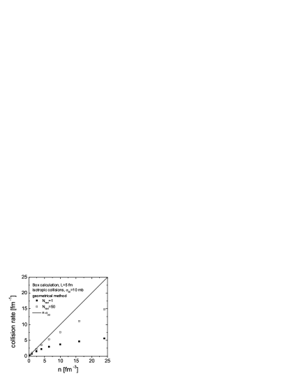
Figure 2: Collision rates for given particle densities. The size of the box is $5$ fm $\times$ $5$ fm $\times$ $5$ fm. We apply here the geometrical collision algorithm. The collisions are isotropic and the total cross section is fixed to a constant $\sigma_{22}=10$ mb. The particle system is taken initially as thermal with a temperature of $T=1$ GeV. The solid line shows the expected relationship between collision rate and particle density: $R=n\sigma_{22}$. The solid squares show the calculated collision rates without test particles ($N_{test}=1$) and the open squares show the results with $50$ test particles per real particle ($N_{test}=50$).

Such a successful passing of the previous test is necessary for every collision algorithm, but it is still not a sufficient argument to guarantee whether the presented algorithm is operating correctly. One has to ask any numerical algorithm for its limitation of correctly describing the underlying problem. To be specific when considering the collision integral (II), it is not obvious whether the geometrical interpretation of the total cross section is a reasonable choice to account for the Boltzmann process. In fact such a description has some shortcomings concerning causality violations which have been pointed out for example in Ref. [35]. Especially for the algorithm presented above we have to face the fact that the collision times of colliding particles are different in the lab frame. This will lead to a noticeable reduction of the collision rate compared to one given by the collision integral: Assume that the difference of the collision times is $\Delta t_{c}$. Consequently the particle with larger collision time should not collide again during this interval $\Delta t_{c}$, otherwise causality would be violated. As pointed out in Appendix A, for a system in equilibrium the ensemble averaged time delay $<\Delta t_{c}>$ depends only on the total cross section and increases with the increasing total cross section. This will lead to an artificial increase of the mean free path and thus to a decrease of the collision rate. In other words, the collision rate decreases when noncausal collisions are forbidden. This problem has also been pointed out in Ref. [36, 37]. We can demonstrate this effect employing box calculations, in which we consider an initially kinetic equilibrated gas distributed homogenously within the box. The size of the box is taken to be the same as in Fig. 1. We employ isotropic collisions with a constant cross section of $\sigma_{22}=10$ mb. In Fig. 2 collision rates are depicted as solid squares for several particle densities. The collision rate is obtained here as the time average of the collision number. While the box size is fixed, we vary the particle number to get different densities. The solid line shows the expected relationship between the collision rate and particle density in equilibrium $R=n\sigma_{22}$. We see a clear decrease of the collision rate when the expected mean free path $1/n\sigma_{22}$ is not much larger than the interaction length $\sqrt{\sigma_{22}/\pi}$. Such a numerical artifact would strongly slow down the kinetic thermalization of an initially highly nonequilibrium state, as, for instance, in case of ultrarelativistic heavy ion collisions. As also clearly seen from Fig. 2, the collision rate tends to saturate at high density. The reason for this is that the collision rate has an upper limit which is exactly the inverse of the average collision time difference $<\Delta t_{c}>/2$ depending only on the total cross section as mentioned before. One can compute $<\Delta t_{c}>/2$ analytically. The detailed calculation is given in Appendix A. It turns out that $<\Delta t_{c}>/2=0.12$ fm/c for $\sigma_{22}=10$ mb. This indicates that the saturation value of the collision rate would be $8.3$ $\mbox{fm}^{-1}$ at high density.

We now return to the slight discrepancy at low energy as noticed in Fig. 1 and consider this as a consequence of the same effect of the relativistic time spread of collisions pointed out above, since in this particular situation the particle density is so high that the mean free path is one order of magnitude smaller than the interaction length. To confirm this suspicion, we carry out similar calculations as in Fig. 1, but with a tiny cross section of $\sigma_{22}=0.1$ mb. The energy distribution, depicted as thick histogram, is shown in Fig. 3 compared with the distribution (thin histogram) obtained by using $\sigma_{22}=10$ mb. One does not see the artificial distortion in the spectrum at low energies any more when the cross section and hence the relativistic time spread is small. As a conclusion, the relativistic time spread effect not only decreases the collision rate, but also slightly distorts the system out of equilibrium.

To suppress this numerical artifact and hence to conserve Lorentz covariance we employ the widely used test particle, or “subdivision”, technique [38, 39] based on the scaling

$$n\to n\,N_{test}\quad\mbox{and}\quad\sigma\to\sigma/N_{test},$$ (6)

where $N_{test}$ is the number of test particles belonging to one real particle. While the mean free path is unchanged by the scaling, the interaction length is reduced by a factor of $\sqrt{N_{test}}$. This consequently reduces the relativistic time spread which vanishes in the limit $N_{test}\to\infty$. The open squares in Fig. 2 denote the results by using $N_{test}=50$. The tendency of convergency towards the ideal limit is visible.

In Fig. 4 we show the time evolution of the momentum anisotropy defined as the fraction of the average transverse momentum squared over the average longitudinal momentum squared. The initial conditions and parameters are set to be the same as in Fig. 1. The dotted line depicts the result without applying the test particle method ($N_{test}=1$) and the dashed line shows the result with $N_{test}=50$. The results confirm our reasoning that the relativistic effect of spreading of the two collision times for a colliding particle pair increases the relaxation time for achieving kinetic equilibrium.

II.2 The stochastic method

In the last section we have determined the collision probability of two incoming particles by means of the geometrical interpretation of the total cross section. Instead, one can also derive the collision probability directly from the collision term of the Boltzmann equation [40, 41, 42]. When assuming two particles in a spatial volume element $\Delta^{3}x$ with momenta in the range (${\bf p}_{1},{\bf p}_{1}+\Delta^{3}p_{1}$) and (${\bf p}_{2},{\bf p}_{2}+\Delta^{3}p_{2}$), the collision rate per unit phase space for such particle pair can be read off from Eq. (II)

$$\frac{\Delta N_{coll}^{2\to 2}}{\Delta t\frac{1}{(2\pi)^{3}}\Delta^{3}x\Delta^{3}p_{1}} = \frac{1}{2E_{1}}\frac{\Delta^{3}p_{2}}{(2\pi)^{3}2E_{2}}f_{1}f_{2}$$ (7)

$$\times\frac{1}{\nu}\int\frac{d^{3}p^{{}^{\prime}}_{1}}{(2\pi)^{3}2E^{{}^{\prime}}_{1}}\frac{d^{3}p^{{}^{\prime}}_{2}}{(2\pi)^{3}2E^{{}^{\prime}}_{2}}|{\cal M}_{12\to 1^{\prime}2^{\prime}}|^{2}(2\pi)^{4}\delta^{(4)}(p_{1}+p_{2}-p^{{}^{\prime}}_{1}-p^{{}^{\prime}}_{2}).$$

Expressing distribution functions as

$$f_{i}=\frac{\Delta N_{i}}{\frac{1}{(2\pi)^{3}}\Delta^{3}x\Delta^{3}p_{i}},\quad i=1,2,$$ (8)

and employing the usual definition of cross section [46] for massless particles

$$\sigma_{22}=\frac{1}{2s}\frac{1}{\nu}\int\frac{d^{3}p^{{}^{\prime}}_{1}}{(2\pi)^{3}2E^{{}^{\prime}}_{1}}\frac{d^{3}p^{{}^{\prime}}_{2}}{(2\pi)^{3}2E^{{}^{\prime}}_{2}}|{\cal M}_{12\to 1^{\prime}2^{\prime}}|^{2}(2\pi)^{4}\delta^{(4)}(p_{1}+p_{2}-p^{{}^{\prime}}_{1}-p^{{}^{\prime}}_{2})\,,$$ (9)

one obtains the absolute collision probability in a unit box $\Delta^{3}x$ and unit time $\Delta t$

$$P_{22}=\frac{\Delta N_{coll}^{2\to 2}}{\Delta N_{1}\Delta N_{2}}=v_{rel}\sigma_{22}\frac{\Delta t}{\Delta^{3}x}\,.$$ (10)

$v_{rel}=s/2E_{1}E_{2}$ denotes the relative velocity, where $s$ is the invariant mass of the particle pair. Unlike in the geometrical method where the collision probability is either $0$ or $1$, $P_{22}$ now can be any number between $0$ and $1$. (Notice that, in practice, one should choose suitable $\Delta^{3}x$ and $\Delta t$ to make $P_{22}$ to be consistently less than $1$.) Whether the collision will happen or not is sampled stochastically as follows: We compare $P_{22}$ with a random number between $0$ and $1$. If the random number is less than $P_{22}$, the collision will occur. Otherwise there is no collision between the two particles within the present time step. We call this collision algorithm the “stochastic method”. Since in the limit $\Delta t\to 0$ and $\Delta^{3}x\to 0$ the numerical solutions using the stochastic method converge to the exact solutions of the Boltzmann equation [47], we divide in practice the space into sufficient small spatial cells. For a true situation $\Delta t$ and $\Delta^{3}x$ have to be taken smaller than the typical scales of spatial and temporal inhomogeneities of the particle densities. Only particles from the same cell can collide with each other. If a particle pair collides, the collision time will be sampled uniformly within the interval ($t,t+\Delta t$). The collision times for both colliding particles are here the same. The particle system propagates now from one time step to the next. This is different compared to the transport simulation scheme utilizing the geometrical method.

In general we also might employ, in addition, the test particle technique in order to reduce statistical fluctuations of the collision events in cells. Accordingly the collision probability is changed to

$$P^{{}^{\prime}}_{22}=v_{rel}\frac{\sigma_{22}}{N_{test}}\frac{\Delta t}{\Delta^{3}x}$$ (11)

by the scaling $\sigma\to\sigma/N_{test}$.

In the following we discuss the Lorentz invariance of the stochastic algorithm in the limit $\Delta^{3}x\to 0$, $\Delta t\to 0$ and $N_{test}\to\infty$. Since $\Delta t\Delta^{3}x$, $\Delta^{3}p/\Delta E$, the distribution function $f$ and the total cross section are Lorentz scalars, it is easy to realize from Eq. (7) that the collision number $\Delta N_{coll}^{2\to 2}$ is a scalar under Lorentz transformations. Furthermore this is also true for $\Delta N_{i}$, the particle number counted within a phase space interval at time $t$. Hence, the collision rate $\Delta N_{coll}^{2\to 2}/\Delta N_{i}\Delta\tau$ as well as the collision probability $P_{22}$ are scalars under Lorentz transformations. Therefore, in the limit $\Delta^{3}x\to 0$, $\Delta t\to 0$ and $N_{test}\to\infty$ the stochastic method yields per se a Lorentz covariant algorithm. However, in practice, a non-zero subvolume $\Delta^{3}x$ and a non-zero timestep $\Delta t$ disturb full Lorentz invariance explicitely. Any potential, but unphysical frame dependence will be discussed later in Sec. V.

To test and demonstrate the stochastic method we again pursue box calculations. The initial conditions are the same as in Fig. 1. The size of the box is set as before to be $5$ fm $\times$ $5$ fm $\times$ $5$ fm. Since we consider a spatially homogeneous initial situation of particles and this configuration will not change very much during particle propagation, we choose a straightforward static cell configuration and divide the box into equal cells. The cell length is set to be $1$ fm in the calculations. We consider isotropic collisions and use a constant total cross section of $\sigma_{22}=10$ mb. Figure 5 shows the final energy distribution obtained by an average over $50$ independent runs (with $N_{test}=1$). One clearly recognizes that the stochastic collision algorithm also passes this basic test. The agreement between the numerical and analytical distribution is perfect and we do not see any distortion in the spectrum in contrast to the situation experienced in Fig. 1.

Since the stochastic method is based directly on the formal collision rate, thus the numerical realized collision rate should be met in transport simulations if the sampled statistics in each cell is sufficiently high. We extract the collision rates from box calculations employing the stochastic method and show the results in Fig. 6 as solid squares. The box size and cell configuration are set to be the same as in Fig. 5. The system is taken at thermal equilibrium for the initial condition. One nicely recognizes that the squares lay on the expected line. (We do mention here that the box size is fixed and we vary the particle number to simulate different particle densities. For instance, a density of $1$ $\mbox{fm}^{-3}$ corresponds to a total particle number of $125$, which means on average one particle per cell. For still lower densities not investigated, one would have to work in addition with a suitable amount of test particles.)

For a system which is initially out of equilibrium the lack of statistics in cells will affect the dynamical evolution of the system, since now all cells are correlated during the relaxation time. To study the effect we repeat the same simulations performed for Fig. 5 starting with that particular nonequilibrium initial condition (5) and calculate the time evolution of momentum anisotropy. We use here the test particle method to control statistical fluctuations. Figure 7 shows the time evolution of the anisotropy for different test particle numbers $N_{test}$. We see that the lack of statistics in cells leads to a slight slowdown in the momentum relaxation. This effect is reduced by using larger values for $N_{test}$, which in turn results in lower statistical fluctuations.

Let us summarize with some comparisons between the two simulation methods of treating collisions as presented in this section. In the simulation employing the stochastic method, the collision rate is correctly realized if the statistics in the individual cell is sufficiently high. In contrast, the collision rate will be numerically suppressed in the simulation using the geometrical method, when the mean free path is not much larger than the interaction length among test particles. In simulations with both algorithms the test particle technique has to be applied in addition in order to solve the Boltzmann equation with sufficient accuracy. For dense and strongly interacting system, convergence of the numerical results with increasing test particle number turns out to be more efficient in simulations employing the stochastic method than in simulations employing the geometrical method, as shown in Fig. 4. In transport simulations applying the stochastic method we have to face the difficulty of dynamically configurating the space into small cells, which is not necessary in the geometrical method. Furthermore, the time step has to be chosen much smaller than the cell volume to avoid a strong change of the density distribution in cells. This, of course, reduces the computing efficiency. In general one should choose such a collision algorithm, so that numerical expense is small. However, the stochasic method offers an advanced technique when dealing with inelastic collision processes, which is the subject of the next section, whereas it might be rather impossible to get a unique and consistent geometrical picture for multiparticle transition processes like $2\leftrightarrow 3$ for instance. A further comparison between the two algorithms will be discussed in Sec. V concerning any potential, but unphysical Lorentz frame dependence of the algorithms.

III Particle multiplication and annihilation processes

In this section we will now immediately extend the stochastic method to the more complicated particle multiplication and annihilation processes involving more than two particles. These processes are essential to drive the system towards chemical equilibrium and also do contribute to kinetic equilibration. The simplest processes are $2\leftrightarrow 3$. In physical terms such processes will be specified then later in the paper as gluon Bremsstrahlung and its back reaction. We note that the stochastic method has already been employed for $2\leftrightarrow 3$ processes in deuteron production $pnN\leftrightarrow dN$ [40] and antibaryon production via, e.g., $\rho+\rho+\omega\leftrightarrow\bar{B}+B$ [42] with much simpler and factorized matrix elements. The true complication in the following is to incorporate the true Bremsstrahlung matrix element. Now we will discuss their numerical implementations. The implementation of higher order processes is straightforward within the extended stochastic algorithm.

The collision term corresponding the $2\leftrightarrow 3$ processes of identical particles is given by the expression

$${\cal C}_{23} = \frac{1}{2E_{1}}\frac{1}{2!}\int\frac{d^{3}p_{2}}{(2\pi)^{3}2E_{2}}\frac{d^{3}p_{3}}{(2\pi)^{3}2E_{3}}\,\frac{1}{2!}\int\frac{d^{3}p^{\prime}_{1}}{(2\pi)^{3}2E^{\prime}_{1}}\frac{d^{3}p^{\prime}_{2}}{(2\pi)^{3}2E^{\prime}_{2}}\times$$ (12)

$$\times f^{\prime}_{1}\,f^{\prime}_{2}\,|{\cal M}_{1^{\prime}2^{\prime}\to 123}|^{2}\,(2\pi)^{4}\,\delta^{(4)}(p^{\prime}_{1}+p^{\prime}_{2}-p_{1}-p_{2}-p_{3})$$

$$+\frac{1}{2E_{1}}\int\frac{d^{3}p_{2}}{(2\pi)^{3}2E_{2}}\,\frac{1}{3!}\int\frac{d^{3}p^{\prime}_{1}}{(2\pi)^{3}2E^{\prime}_{1}}\frac{d^{3}p^{\prime}_{2}}{(2\pi)^{3}2E^{\prime}_{2}}\frac{d^{3}p^{\prime}_{3}}{(2\pi)^{3}2E^{\prime}_{3}}\times$$

$$\times f^{\prime}_{1}\,f^{\prime}_{2}\,f^{\prime}_{3}\,|{\cal M}_{1^{\prime}2^{\prime}3^{\prime}\to 12}|^{2}\,(2\pi)^{4}\,\delta^{(4)}(p^{\prime}_{1}+p^{\prime}_{2}+p^{\prime}_{3}-p_{1}-p_{2})$$

$$-\frac{1}{2E_{1}}\frac{1}{2!}\int\frac{d^{3}p_{2}}{(2\pi)^{3}2E_{2}}\frac{d^{3}p_{3}}{(2\pi)^{3}2E_{3}}\,\frac{1}{2!}\int\frac{d^{3}p^{\prime}_{1}}{(2\pi)^{3}2E^{\prime}_{1}}\frac{d^{3}p^{\prime}_{2}}{(2\pi)^{3}2E^{\prime}_{2}}\times$$

$$\times f_{1}\,f_{2}\,f_{3}\,|{\cal M}_{123\to 1^{\prime}2^{\prime}}|^{2}\,(2\pi)^{4}\,\delta^{(4)}(p_{1}+p_{2}+p_{3}-p^{\prime}_{1}-p^{\prime}_{2})$$

$$-\frac{1}{2E_{1}}\int\frac{d^{3}p_{2}}{(2\pi)^{3}2E_{2}}\,\frac{1}{3!}\int\frac{d^{3}p^{\prime}_{1}}{(2\pi)^{3}2E^{\prime}_{1}}\frac{d^{3}p^{\prime}_{2}}{(2\pi)^{3}2E^{\prime}_{2}}\frac{d^{3}p^{\prime}_{3}}{(2\pi)^{3}2E^{\prime}_{3}}\times$$

$$\times f_{1}\,f_{2}\,|{\cal M}_{12\to 1^{\prime}2^{\prime}3^{\prime}}|^{2}\,(2\pi)^{4}\,\delta^{(4)}(p_{1}+p_{2}-p^{\prime}_{1}-p^{\prime}_{2}-p^{\prime}_{3})\,.$$

The collision probability $P_{23}$ for a particle multiplication process can be derived analogously to Eq. (10) as

$$P_{23}=v_{rel}\frac{\sigma_{23}}{N_{test}}\frac{\Delta t}{\Delta^{3}x},$$ (13)

where the total cross section $\sigma_{23}$ is defined as

$$\sigma_{23}=\frac{1}{2s}\frac{1}{3!}\int\frac{d^{3}p^{{}^{\prime}}_{1}}{(2\pi)^{3}2E^{{}^{\prime}}_{1}}\frac{d^{3}p^{{}^{\prime}}_{2}}{(2\pi)^{3}2E^{{}^{\prime}}_{2}}\frac{d^{3}p^{{}^{\prime}}_{3}}{(2\pi)^{3}2E^{{}^{\prime}}_{3}}|{\cal M}_{12\to 1^{\prime}2^{\prime}3^{\prime}}|^{2}(2\pi)^{4}\delta^{(4)}(p_{1}+p_{2}-p^{{}^{\prime}}_{1}-p^{{}^{\prime}}_{2}-p^{{}^{\prime}}_{3}).$$ (14)

One can also extend the geometrical method to the multiplication processes. But it is in general impossible to obtain a unified scheme for the annihilation processes in a consistent geometrical picture. In contrast, the extension to $3\to 2$ processes via the stochastic method is straightforward. We write the collision rate stemming from Eq. (12) per unit phase space in a form like Eq. (7)

$$\frac{\Delta N_{coll}^{3\to 2}/N_{test}}{\Delta t\frac{1}{(2\pi)^{3}}\Delta^{3}x\Delta^{3}p_{1}} =\frac{1}{2E_{1}}\frac{\Delta^{3}p_{2}}{(2\pi)^{3}2E_{2}}\frac{\Delta^{3}p_{3}}{(2\pi)^{3}2E_{3}}\frac{f_{1}}{N_{test}}\frac{f_{2}}{N_{test}}\frac{f_{3}}{N_{test}}$$

$$\times\frac{1}{2!}\int\frac{d^{3}p^{{}^{\prime}}_{1}}{(2\pi)^{3}2E^{{}^{\prime}}_{1}}\frac{d^{3}p^{{}^{\prime}}_{2}}{(2\pi)^{3}2E^{{}^{\prime}}_{2}}|{\cal M}_{123\to 1^{\prime}2^{\prime}}|^{2}(2\pi)^{4}\delta^{(4)}(p_{1}+p_{2}+p_{3}-p^{{}^{\prime}}_{1}-p^{{}^{\prime}}_{2})\,,$$

where $f_{i},i=1,2,3,$ denote now the phase space density of the test particles. Inserting Eq. (8) into Eq. (III) gives the collision probability of a $3\to 2$ process

$$P_{32}=\frac{\Delta N_{coll}^{3\to 2}}{\Delta N_{1}\Delta N_{2}\Delta N_{3}}=\frac{1}{8E_{1}E_{2}E_{3}}\frac{I_{32}}{N_{test}^{2}}\frac{\Delta t}{(\Delta^{3}x)^{2}}$$ (16)

for given momenta of the incoming particles in a particular space cell. $I_{32}$ is defined as the integral $\frac{1}{2!}\int d^{3}p^{\prime}_{1}d^{3}p^{\prime}_{2}\cdots$ in Eq. (III) over the final states.

Danielewicz and Bertsch [40] obtained a similar expression for $P_{32}$

$$P_{32}=v_{12}\frac{\sigma_{12}}{N_{test}}\frac{{\cal V}_{3}}{N_{test}}\frac{\Delta t}{(\Delta^{3}x)^{2}},$$ (17)

when investigating the production of deuterons in a nonrelativistic transport model of low energy heavy ion reactions, where they approximately factorized the matrix element into a term describing a two-body collision and a term mimicking particle fusion. $\sigma_{12}$ is the total cross section for the two-body collision and ${\cal V}_{3}$ can be interpreted as a volume: Once three particles are within this volume, a $3\to 2$ transition may be considered to occur. The volume scales with ${\cal V}_{3}\to{\cal V}_{3}/N_{test}$ when employing test particles. Therefore it is intuitively clear why the quantity $I_{32}$ in Eq. (16) scales with $1/N^{2}_{test}$. In contrast to Eq. (17), expression (16) is a more general one formulated in a unified manner, and is correct for any given matrix elements without any approximations.

As an example, when considering isotropic $2\leftrightarrow 3$ collisions for identical particles, integrals over momentum space for $\sigma_{23}$ and $I_{32}$ can be easily calculated analytically and one obtains

$$I_{32}=192\pi^{2}\sigma_{23}\,.$$ (18)

Applying the probabilities (13) and (16) we are now able to study kinetic and chemical equilibration in a box. We assume a system consisting of identical particles and consider only isotropic $2\leftrightarrow 3$ collisions. $\sigma_{23}$ is set to be $10$ mb. As in the box calculations refering to Fig. 1, initially the system is chosen to be strongly out of equilibrium according to Eq. (5). The particles are distributed homogeneously in the box. The box has a volume of $5$ fm $\times$ $5$ fm $\times$ $5$ fm and is divided into equal cells. The cell length is $1$ fm. Initially the system contains $N_{0}=2000$ massless particles. Newly produced particles will be positioned randomly within the individual cells where the transitions occur. Before we come to the results, let us determine the final particle density and temperature to be expected when the system becomes thermally equilibrated. For an ultrarelativistic (one component) Maxwell-Boltzmann gas the following relations

$$\epsilon=3n_{eq}T\quad\mbox{and}\quad n_{eq}=\frac{T^{3}}{\pi^{2}}$$ (19)

hold in equilibrium. One can solve $T$ and $n_{eq}$ for an energy density given by the initial condition. In our case, according to Eq. (5), we obtain $T=1.248$ GeV and $n_{eq}=25.64$ $\mbox{fm}^{-3}$ which is larger than the initial particle density $n(t_{0})=16$ $\mbox{fm}^{-3}$. Figure 8 depicts the time evolution of the particle density obtained from the box calculation. The results are obtained by averaging ten independent runs. We see that the particle density increases smoothly towards its final value which agrees fully with the analytical expectation. The dotted curve presents an estimate made by using the following relaxation approximation

$$n(t)=n_{eq}+(n(t_{0})-n_{eq})\ e^{-\frac{t-t_{0}}{\theta}},$$ (20)

where $\theta$ stands for the relaxation time. In general, for any complex equilibration, this quantity will be time dependent. For the estimate the relaxation time is taken by a simple fixed value at equilibrium $\theta=1/n_{eq}\sigma_{23}$ which slightly overestimates the relaxation, as also seen in Fig. 8. In Fig. 9 the final energy distribution is depicted by the histogram. The dotted line denotes the analytical distribution with the expected temperature $T=1.248$ GeV. The numerical result agrees again perfectly with the analytical distribution. The fact that the final particle density and the final temperature obtained from the inverse slope of the energy spectrum are identical to the two analytical values demonstrates that detailed balance between the multiplication and annihilation processes is fully realized in our simulations. In Fig. 10 we compare the time evolutions of the normalized particle density (the fugacity) and the momentum anisotropy. It turns out that for the given initial conditions the kinetic equilibration is slightly slower compared to the chemical equilibration. We notice that the quantity $2<p_{z}^{2}>/<p_{T}^{2}>=2\int{d^{3}p\,p_{z}^{2}\,f}/\int{d^{3}p\,p_{T}^{2}\,f}$ is more sensitive to fluctuations than $n=\int{d^{3}p/(2\pi)^{3}\,f}$, which is the reason why in Fig. 10 the curve of the fugacity is smoother than that of the momentum anisotropy.

IV Quark Gluon Plasma in box

A quark gluon plasma (QGP) is suggested as a kineticly and chemically equilibrated system of deconfined quarks and gluons. Such state of matter is presumed to have been formed after the big bang and also expected to exist temporarily during the course of an ultrarelativistic heavy ion collision in the laboratory. The main goal of the heavy ion collision experiments at RHIC and of the future experiments at LHC is to find evidence of such a new state of matter, the existence of quark gluon plasma. From the theoretical point of view it is also very interesting to address the possibility of the formation of QGP under different theoretical assumptions of the initial conditions, and to investigate the further evolution of the quark gluon system in space and time. A cascade type transport simulation solving relativistic Boltzmann equations for quarks and gluons with Monte Carlo technique is just well suited for such a study. Whereas the current parton cascade models, MPC [24], PCPC [25] and VNI/BMS [26], have not included the $2\leftrightarrow 3$ processes, we can apply the extended stochastic collision algorithm presented in the last section to build up a parton cascade describing the space-time evolution of interacting quarks and gluons including $gg\leftrightarrow ggg$ within the framework of perturbative QCD. As a first application, we restrict ourselves in this section to investigate the formation of a quark gluon plasma in a fixed box. The convenience is that a thermalized parton system should be formed in any case after some time. Although this situation cannot be given in reality, one can still address the way of equilibration for different particle species. Furthermore, box calculations offer an essential test for the numerical realization of detailed balance of $gg\leftrightarrow ggg$ and $gg\leftrightarrow q\bar{q}$ processes. A realistic space-time approach for the simulation of parton evolution during the early stage after an ultrarelativistic heavy ion collision will be presented in Sec. VI.

The parton interactions include all two-body processes: ($1$) $gg\leftrightarrow gg$, ($2$) $gg\leftrightarrow q{\bar{q}}$ ($3$) $gq\leftrightarrow gq$, ($4$) $qq\leftrightarrow qq$, ($5$) $qq^{\prime}\leftrightarrow qq^{\prime}$, ($6$) $q{\bar{q}}\leftrightarrow q{\bar{q}}$, ($7$) $q{\bar{q}}\leftrightarrow q^{\prime}{\bar{q}^{\prime}}$, and three-body processes ($8$) $gg\leftrightarrow ggg$. The matrix elements squared in leading order of the perturbative QCD are taken from Refs. [48, 49]. We regularize the infrared divergences by using the Debye screening mass [21] $m_{D}^{2}$ for gluons

$$m_{D}^{2}=16\pi\alpha_{s}\int\frac{d^{3}p}{(2\pi)^{3}}\frac{1}{p}(N_{c}f_{g}+n_{f}f_{q})$$ (21)

and the quark medium mass $m_{q}^{2}$ for quarks

$$m_{q}^{2}=4\pi\alpha_{s}\frac{N_{c}^{2}-1}{2N_{c}}\int\frac{d^{3}p}{(2\pi)^{3}}\frac{1}{p}(f_{g}+f_{q}),$$ (22)

where $N_{c}=3$ for SU(3) of QCD and $n_{f}$ is the number of quark flavor. All formulas for the differential cross sections are listed in Appendices C and D. Here we write down only the differential cross sections (or the matrix element squared) of the dominant processes for achieving kinetic and chemical equilibration [20, 31]:

$$\frac{d\sigma^{gg\to gg}}{dq_{\perp}^{2}}=\frac{9\pi\alpha_{s}^{2}}{(q_{\perp}^{2}+m_{D}^{2})^{2}}\,,$$ (23)

$$\frac{d\sigma^{gg\to q\bar{q}}}{dq_{\perp}^{2}}=\frac{\pi\alpha_{s}^{2}}{3s(q_{\perp}^{2}+m_{q}^{2})}\,,$$ (24)

$$|{\cal M}_{gg\to ggg}|^{2}=\left(\frac{9g^{4}}{2}\frac{s^{2}}{({\bf q}_{\perp}^{2}+m_{D}^{2})^{2}}\right)\left(\frac{12g^{2}{\bf q}_{\perp}^{2}}{{\bf k}_{\perp}^{2}[({\bf k}_{\perp}-{\bf q}_{\perp})^{2}+m_{D}^{2}]}\right)\,,$$ (25)

where $g^{2}=4\pi\alpha_{s}$. The matrix element (25) describing the $gg\leftrightarrow ggg$ transitions is factorized into a part for elastic scattering and a part for gluon radiation (or gluon fusion). ${\bf q}_{\perp}$ and ${\bf k}_{\perp}$ denote, respectively, the perpendicular component of the momentum transfer and that of the momentum of the radiated gluon in the c.m. frame. In a dense medium the radiation of soft gluons is assumed to be suppressed due to the Landau-Pomeranchuk effect: The emission of a soft gluon should be completed before it scatters again. This leads to a lower cutoff of $k_{\perp}$ via a step function $\Theta(k_{\perp}\Lambda_{g}-\cosh y)$, where $y$ is the rapidity of the radiated gluon in the c.m. frame and $\Lambda_{g}$ denotes the gluon mean free path which is the inverse of the gluon collision rate $\Lambda_{g}=1/R_{g}$. $R_{g}$ is the sum of the rate of the following transitions: $gg\to gg$, $gg\to q{\bar{q}}$, $gq\to gq$, $gg\to ggg$, and $ggg\to gg$.

The collision rate is an important quantity governing the time scale of kinetic and chemical equilibration. In Fig. 11 we depict the thermally averged cross section $<v_{rel}\sigma>$ and the gluon collision rates as function of temperature for $gg\to gg$, $gg\to q{\bar{q}}$, $gq\to gq$, and $gg\to ggg$ transitions. $<v_{rel}\sigma>$ are calculated numerically, for which we take the screening masses obtained at equilibrium ($f_{g}=f_{q}=e^{-E/T}$)

$$m_{D}^{2}=(3+n_{f})\frac{8}{\pi}\alpha_{s}T^{2}\quad\mbox{and}\quad m_{q}^{2}=\frac{16}{3\pi}\alpha_{s}T^{2}\,.$$ (26)

In the calculations we consider two quark flavors ($n_{f}=2$) and employ a constant coupling $\alpha_{s}=0.3$. The corresponding collision rates are obtained by $R=n_{g}<v_{rel}\sigma>$, where $n_{g}=\nu_{g}T^{3}/\pi^{2}$ is the gluon density in thermal equilibrium. $\nu_{g}=2\times 8$ denotes the degeneracy of gluons. Because of our simple minded inclusion of the Landau-Pomeranchuk effect, the cross section $\sigma_{gg\to ggg}$ depends on the sum of the rates $R_{g}=R_{gg\to gg}+R_{gg\to q{\bar{q}}}+R_{gg\to ggg}+R_{ggg\to gg}$, in which, however, $R_{gg\to ggg}$ and $R_{ggg\to gg}(=R_{gg\to ggg}\mbox{ in equilibrium})$ depend again on $\sigma_{gg\to ggg}$. This problem is solved by a selfconsistent, iterative computation. Inspecting Fig. 11 we see that the collision rates are proportional to the temperature, which indicates that the $<v_{rel}\sigma>$ are inversely proportional to $T^{2}$. This behavior stems from the fact that the cross section $\sigma_{gg\to gg}$ and $\sigma_{gq\to gq}$ depend mainly on $1/m^{2}_{D}$ and the cross section $\sigma_{gg\to ggg}$ and $\sigma_{gg\to q{\bar{q}}}$ mainly on $1/s$. Furthermore we realize that the collision rate of the three-body processes is in the same order as the rate of two-body gluon collisions.

We now come to some numerical details when simulating the parton equilibration in a fixed box. As shown in Appendix D, the computations of $\sigma_{23}$ and $I_{32}$ over momentum space are reduced to a four- (95) and a two-dimensional (99) integration respectively. Even then, the computations are still time-consuming when $\sigma_{23}$ and $I_{32}$ have to be calculated for every gluon doublet and triplet in cells, since the number of integrations is proportional to $n^{2}$ and $n^{3}$ respectively ($n$ being the total gluon number in an individual cell). In order to reduce the computing time, one first thinks of tabulating $\sigma_{23}$ as well as $I_{32}$. In simulations we then make interpolations using these tabulated data sets. This gives a convenient way for obtaining $\sigma_{23}$ because the underlying integral depends on only two parameters, $m_{D}^{2}/s$ and $\Lambda_{g}\sqrt{s}$, as mentioned in Appendix D. The same data sets have been used for calculating $\sigma_{23}$ in thermal equilibrium as shown in Fig. 11. In contrast to the case for $\sigma_{23}$, $I_{32}$ depends on five parameters (see Appendix D). A tabulation of $I_{32}$ is thus crude due to the limitation of the storage, which leads to large errors by interpolations. Therefore we decide to calculate $I_{32}$ in simulations using the Monte Carlo algorithm VEGAS [50] with low computing expense (two iterations and $100$ function calls). Furthermore, instead of evaluating probabilities of all possible collisions, we follow the scheme of Refs. [40, 41] and choose randomly ${\cal N}$ out of the possible doublets or triplets, since in our case the transition probabilities of any channel are in fact very small within one time step. In order to achieve the correct collision rate, we have to accordingly amplify the corresponding collision probabilities to be

$$P_{22}\to P_{22}\frac{n(n-1)/2}{{\cal N}_{22}}\,,\quad P_{23}\to P_{23}\frac{n(n-1)/2}{{\cal N}_{23}}\,,\quad P_{32}\to P_{32}\frac{n(n-1)(n-2)/6}{{\cal N}_{32}}\,.$$ (27)

The choices of ${\cal N}_{22}$, ${\cal N}_{23}$ and ${\cal N}_{32}$ are arbitrary. In the following simulations we set ${\cal N}_{22}={\cal N}_{23}={\cal N}_{32}=n$.

The initial condition for the box calculations is taken by sampling multiple minijet production in heavy ion collisions at RHIC energy $\sqrt{s}=200$ GeV. Minijets denote on-shell partons with transverse momentum being greater than $p_{0}$, where $p_{0}$ is a parameter separating the hard, perturbative, from the soft, nonperturbative, nucleon interactions. In calculations we set $p_{0}$ to be $2$ GeV. It had been proposed a long time ago in Ref. [44] that at RHIC energy the produced minijets take half of the transverse energy. The momentum spectrum of the minijets has a power-law behavior and thus the initial condition of the minijets is strongly out of equilibrium. In the following studies we are interested in the way of how thermalization of different parton species proceeds and also interested in the timescales of kinetic and chemical equilibration.

We assume that a nucleus-nucleus collision can be simply modeled as a sequence of binary nucleon-nucleon collisions. Then the initial momentum distribution of the produced partons is obtained according to the differential jet cross section in nucleon-nucleon collisions [51]

$$\frac{d\sigma_{jet}}{dp_{T}^{2}dy_{1}dy_{2}}=K\sum_{a,b}x_{1}f_{a}(x_{1},p_{T}^{2})x_{2}f_{b}(x_{2},p_{T}^{2})\frac{d\sigma_{ab}}{d\hat{t}}\,,$$ (28)

where $p_{T}$ is the transverse momentum and $y_{1}$ and $y_{2}$ are the momentum rapidities of the produced partons. $x_{1}$ and $x_{2}$ are the Feynman variables denoting the longitudinal momentum fractions carried by the partons respectively. $d\sigma_{ab}$ stands for the leading order perturbative parton-parton cross sections. The phenomenological factor $K$, set to be $2$, accounts for higher-order corrections. We employ the Glück-Reya-Vogt parametrization [52] for the parton structure functions $f_{a}(x,p_{T}^{2})$. For the box calculations we consider gluons stremming from a central rapidity region $y\in[-0.5:0.5]$ as the only initial parton species, since at the central rapidity region the partons with small $x$ dominate and these are almost gluons. The initial number of gluons is assumed to be $500$.

The primary minijets produced in a real high energy heavy ion collision are distributed within a thin disc due to the Lorentz contraction. Instead of such a space-time configuration, we assume a homogeneous spatial distribution of partons in the box for simplicity. This allows us to still use a static cell configuration. Moreover, all particles are assumed to be formed at t=0 fm/c. We will discuss the space-time distribution of the primary minijets later in Sec. VI when considering the parton evolution in a real heavy ion collision. The size of the box is set to be $3$ fm $\times$ $3$ fm $\times$ $3$ fm and the box is divided into equal cells. The length of a cell is set to be $1$ fm. These settings are tuned as that there will be enough gluons (about $15$) in each cell during the whole evolution. (For quarks strong statistic fluctuation occurs at the beginning of the evolution due to the initial lack of quarks.)

We employ a constant coupling of $\alpha_{s}=0.3$ in the rest of this section for evaluating the screening masses and the cross sections. The screening masses $m_{D}^{2}$ and $m_{q}^{2}$ are calculated dynamically according to Eqs. (21) and (22). The integrations are computed as

$$\int\frac{d^{3}p}{(2\pi)^{3}\,p}\,f\to\frac{1}{V}\sum_{i}\frac{1}{p_{i}}\,,$$ (29)

where the sum runs over all particles in a volume $V$, which should be, in general, small in order to maintain the local homogeneity. Since the initial position of partons is distributed homogeneously, we extend the sum over all particles in the fixed box.

The gluon collision rate, which will be employed for evaluating $\sigma_{23}$ and $I_{32}$, can be obtained from the calculated collision probabilities, since the sum of the probabilities of all possible collisions gives the average total collision number within the current time step. We then have

$$R_{gg\to f}=\frac{\sum_{i}P_{i}^{gg\to f}}{\frac{1}{2}N_{g}\Delta t}\,,\qquad f=gg,q{\bar{q}},ggg,$$ (31)

$$R_{ggg\to gg}=\frac{\sum_{i}P_{i}^{ggg\to gg}}{\frac{1}{2}N_{g}\Delta t}$$

and $$R_{gq\to gq}=\frac{\sum_{i}P_{i}^{gq\to gq}}{N_{g}\Delta t}\,,$$ (32)

where the sums run over possible particle doublets or triplets in the individual cells and also over all cells. $N_{g}$ denotes the total gluon number in the box. On the other hand, the $P_{i}^{gg\to ggg}$ and $P_{i}^{ggg\to gg}$ depend again on $\sigma_{23}$ and $I_{32}$ respectively. Therefore, a correct calculation for $\sigma_{23}$ and $I_{32}$ as well as $P_{i}^{gg\to ggg}$ and $P_{i}^{ggg\to gg}$ should be a selfconsistent, iterative computation. However, since such computations are too time consuming, we employ the gluon collision rate, obtained at the last time step, to calculate $\sigma_{23}$ and $I_{32}$ within the current time step.

When the parton system becomes fully equilibrated at the later evolution, the final values of gluon and quark number should be given by

$$N^{eq}_{g}=\nu_{g}\frac{T^{3}}{\pi^{2}}V\,,$$ (33)

$$N^{eq}_{q}=2\nu_{q}\frac{T^{3}}{\pi^{2}}V\,,$$ (34)

where $\nu_{g}=2\times 8$ and $\nu_{q}=2\times 3\times n_{f}$ are the degeneracy factors of a gluon and quark respectively. The factor $2$ in Eq. (34) indicates the sum of quark and antiquark. Employing the relation

$$E=3(N^{eq}_{g}+N^{eq}_{q})T\,,$$ (35)

which holds in thermal equilibrium, we obtain the final temperature

$$T=\left(\frac{E}{V}\frac{\pi^{2}}{3(\nu_{g}+2\nu_{q})}\right)^{\frac{1}{4}}\,.$$ (36)

The total energy $E$ can be determined by the specified initial momentum distribution of minijets, Eq. (28). Considering only up and down quarks ($n_{f}=2$) we get a final temperature of about $430$ MeV and thus $m_{D}^{2}\approx 0.7\mbox{GeV}^{2}$ and $m_{q}^{2}\approx 0.1\mbox{GeV}^{2}$ for $\alpha_{s}=0.3$.

Figure 12 shows time evolutions of the gluon and quark number. Sixty independent realizations are collected to obtain sufficient statistics. We see that the time evolution of the gluon number has two stages. At first the gluon number increases rapidly to a maximum and then relaxes towards its equilibrium value on a slower scale. The quark number starts from zero because of the initial absence of quark species and increases smoothly towards its equilibrium value. The gluon and quark number do reach their final values simultaneously. These behaviors of $N_{g}(t)$ and $N_{q}(t)$ reveal the well-known scenario of two-stage chemical equilibration: The gluon system equilibrates at first as if no quarks were there and then cools down gradually by producing quark-antiquark pairs until the quarks reach the equilibrium. Such two-stage equilibration could also happen in a real high energy heavy ion collision [53].

Next we compare the equilibrium values of gluon and quark number of Fig. 12 with the analytical values which one would expect directly from the initial conditions. The final temperature in one individual run can be obtained by inserting the total amount of energy into expression (36). Averaged over $60$ runs we have $<T>=427.84$ MeV. Inserting the averaged temperature into Eqs. (33) and (34) gives $<N^{eq}_{g}>=428$ and $<N^{eq}_{q}>=643$. The values extracted from Fig. 12 are $N_{g}=430$ and $N_{q}=640$. We see that the agreements are pretty good, which demonstrates that our new cascade algorithm is indeed very successful in keeping the detailed balance even for the considered complexity of employing pQCD motivated cross sections. We also calculate the equilibrium number of gluons when no quarks are considered ($n_{f}=0$). In the present situation this is $\bar{N}^{eq}_{g}=852$, which is somewhat greater than the maximum of gluon number read off from Fig. 12, since in the latter case gluons are already lost due to the production of quark-antiquark pairs starting at the beginning of the evolution.

In Fig. 13 we depict the energy distributions of the partons (gluons and quarks) at different times. The initial ($t=0$ fm/c) distribution possesses a cutoff at $E=p_{0}=2$ GeV and is highly nonthermal. Immediately after the onset of interactions, soft gluons with smaller energy do emerge by the process $gg\to ggg$ and thermalize very quickly. We see that at $0.3$ fm/c the energy distribution for partons with smaller energy than $2$ GeV is largely populated. The hard particles with larger energy are still out of equilibrium. There is still a hump at $2$ GeV. This hump will vanish gradually and at $2$ fm/c the total distribution becomes exponential. One can refer to this stage as the onset of kinetic equilibration. The energy distribution at a final time of $t=50$ fm/c is also depicted in Fig. 13. We have compared this spectrum to the analytical form Eq. (3) with the averaged temperature $<T>=427.84$ MeV obtained from the initial input. (The analytical distribution is not shown in Fig. 13.) The agreement is very good.

To study the kinetic equilibration in more detail, we calculate the time evolutions of the momentum anisotropy

$$\frac{2<p_{z}^{2}>_{g}}{<p_{T}^{2}>_{g}}(t)\,,\qquad\frac{2<p_{z}^{2}>_{q}}{<p_{T}^{2}>_{q}}(t)$$ (37)

for gluons and quarks, which are shown in Fig. 14. We see that the momentum of the gluons and quarks becomes isotropic at almost same time of about $1-2$ fm/c which is just the timescale when the energy spectrum gets exponential, as shown in Fig. 13. However, if one looks at the time evolutions of the effective temperatures in Fig. 15, which are defined as $T_{g}(t):=E_{g}(t)/3\,N_{g}(t)$ and $T_{q}(t):=E_{q}(t)/3\,N_{q}(t)$, one notices that between $0$ fm/c and $10$ fm/c the temperature of quarks is lower than the one of gluons. The reason is that the quarks stem mainly by the $gg\to q\bar{q}$ quark pair production and the cross section $\sigma_{gg\to q{\bar{q}}}$ is inversely proportional to $s$. Therefore, when the quark production is still more dominant compared to the annihilation process, more quark-antiquark pairs with smaller energies are produced than those with larger energies, compared to the equilibrated Boltzmann distribution. Correspondingly, there would be a slight suppression in the energy spectrum of quarks at high energy and in the energy spectrum of gluons at low energy during the ongoing chemical equilibration. It takes time for the gluon-quark mixture to obtain an identical temperature via the gluon-quark interactions. This identical, final temperature is extracted from Fig. 15, $T_{g}=T_{q}=429$ MeV, and agrees perfectly with the expectation of $<T>=427.84$ MeV.

The parton fugacity is defined as follows

$$\lambda_{g}(t):=\frac{N_{g}(t)}{\tilde{N}^{eq}_{g}(t)}\quad\mbox{and}\quad\lambda_{q}(t):=\frac{N_{q}(t)}{\tilde{N}^{eq}_{q}(t)}\,,$$ (38)

where

$$\tilde{N}^{eq}_{g}(t):=\nu_{g}\frac{T_{g}^{3}(t)}{\pi^{2}}V\quad\mbox{and}\quad\tilde{N}^{eq}_{q}(t):=2\nu_{q}\frac{T_{q}^{3}(t)}{\pi^{2}}V\,.$$ (39)

In Fig. 16 the time evolutions of the fugacity are depicted for gluons (solid curve) and quarks (dotted curve). We see that while the gluons approach the chemical equilibrium at about $3$ fm/c, the quarks do equilibrate later at $20$ fm/c. The two-stage chemical equilibration is clearly demonstrated in Fig. 16.

We also depict the time evolutions of the screening masses in Fig. 17 and of the gluon collision rates in Fig. 18. The comparisons of the extracted equilibrium values from the figures with the analytical values give perfect agreements. In the small window of Fig. 18 the collision rate of $gg\to ggg$(upper) and $ggg\to gg$(lower) are shown by solid lines. We see that the two processes occur with the same rates at about $2\sim 3$ fm/c, which is just the time scale when the gluons become chemically equilibrated. The identical time scale is also obtained from Fig. 16. We did not depict the time evolution of the rate of $ggg\to gg$ process from $3$ fm/c to $50$ fm/c, since it is almost identical with that of $gg\to ggg$ process.

From the present study of creating QGP in a box some speculations are made when we consider parton evolution in a real ultrarelativistic heavy ion collision. (1) Two-stage equilibration is a good scenario describing parton thermalization in high energy heavy ion collisions. (2) The cross section $\sigma_{gg\to ggg}$ is in the same order as $\sigma_{gg\to gg}$ and thus the $gg\leftrightarrow ggg$ processes should play an important role in chemical and as well as kinetic equilibration. Analyses based on a full $3+1$ dimensional transport simulation of the parton evolution after a high energy heavy ion collision will be presented in Sec. VI.

V Testing the frame independence

The relativistic kinetic equation

$$p^{\mu}\partial_{\mu}f=I_{coll}$$ (40)

is a Lorentz covariant expression. Therefore the covariance of its solution should not be affected by the choice of the frame, in which the many-body dynamics is actually described. Frame independence must also be fulfilled for any physical observables which can be expressed as Lorentz scalars. However, the equation (40) cannot be solved exactly in practice by applying a transport algorithm. Strictly speaking, the frame independence is not fulfilled in any cascade-typ simulations. Our aim in this section is to study potential frame dependence in our description employing collision algorithms presented in Secs. II and III. We will also demonstrate the increasing insensitivity of the particularly chosen frame and the convergency of the numerical results when adding more and more test particles into the dynamics.

As explained in Sec. II, the geometrical method is based on the geometrical interpretation of the total cross section and the time ordering of the collision events is generally frame dependent when the mean free path of particles is in the same order as the mean interaction length. In contrast, in simulations employing the stochastic method, which deals with the transition rate, a time ordering of the collision sequence is not needed because collision events will be sampled stochastically within a time step. Still, one has to be aware that a nonzero subvolume of cells and a nonzero timestep disturb the Lorentz invariance. Zhang and Pang had studied already the frame dependence of parton cascade results in Ref. [54] applying a parton cascade code with a similar geometrical collision scheme as presented by us. They argued that results from parton cascade simulations are not sensitive to the choice of the frame when the collision criterion is formulated in the center of mass frame of two incoming partons. We will demonstrate the issues in detail in the following considerations and calculations.

V.1 One dimensional expansion in a tube

For the purpose of studying the frame dependence we do not need consider a special situation. However, as emphasized in the Introduction, the here presented cascade model will be applied to simulate the parton evolution in ultrarelativistic heavy ion collisions. Therefore it makes sense to consider a one dimensional expanding system as testing ground, since at the initial stage of an ultrarelativistic heavy ion collision the partonic system will undergo mainly a longitudinal expansion. For convenience, particles of the test system are classical Boltzmann particles instead of quarks and gluons. Furthermore, in the present section we will employ isotropic collisions and a constant cross section. In order to mimic a perfect longitudinal expansion we embed all particles into a cylindrical tube with infinite length. The reflections of particles against the tube wall are operated in a same way as performed in the box calculations.

Initially, particles are considered to be thermal in their local spatial element. We use a Bjorken-type boost invariant initial conditions [55]

$$f({\mathbf{x}},{\mathbf{p}},\tau)=e^{-\frac{p_{\perp}\cosh(y-\eta)}{T(\tau)}}\,,$$ (41)

where $\tau$ is the proper time $\tau=\sqrt{t^{2}-z^{2}}$ and $y$ and $\eta$ denote, respectively, momentum and space-time rapidity

$$y=\frac{1}{2}\ln\frac{E+p_{z}}{E-p_{z}}\quad,\quad\eta=\frac{1}{2}\ln\frac{t+z}{t-z}\,.$$ (42)

Due to the assumption of the boost invariance, quantities such as particle density $n$, energy density $\epsilon$ and temperature $T$ depend only on the proper time $\tau$. For an ideal, longitudinal and boost-invariant hydrodynamical expansion we obtain

$$n(\tau) = n(\tau_{0})\,\frac{\tau_{0}}{\tau}\,,$$ (43)

$$\epsilon(\tau) = \epsilon(\tau_{0})\,\left(\frac{\tau_{0}}{\tau}\right)^{4/3}\,,$$ (44)

$$T(\tau) = T(\tau_{0})\,\left(\frac{\tau_{0}}{\tau}\right)^{1/3}\,.$$ (45)

Besides the study of the frame dependence we also attempt to address the possibility of buildup of an approximately ideal hydrodynamical expansion in cascade simulations when the collision rate is considered to be very high. The time dependences (43), (44), and (45) then serve as ideal references when comparing them with results extracted from the numerical simulations.

To be able to apply the stochastic method, the tube needs to be subdivided into sufficient small cells. A static cell structure as configurated in the box calculations is not suitable any more for an expanding system. However, since the expansion is only one dimensional, we can still employ a static configuration in the transverse plane. Instead of a lattice structure, (which will also work,) we make use of the symmetry in the given situation and consider a spider web like structure in the transverse plane. Particularly we divide the polar angle $\phi$ and the radial length squared $r^{2}$ equally within the interval $[0,2\pi]$ and $[0,R^{2}]$, respectively, where $R$ denotes the radius of the cylindrical tube. This division gives a same transverse area $\Delta F=\Delta\phi\Delta r^{2}/2$ for all cells. Longitudinally we have to construct a comoving cell configuration which adapts to the expanding system, since, as a reminder, the spatial inhomogeneity of particles in the local cells should be small within one time step. Using the thermal distribution function (41) it can be simply realized by means of the Cooper-Frye formula [56] that the particle number per unit space-time rapidity $dN/d\eta$ calculated at time $t$ in a frame (and also at $\tau$ as well) is constant, i.e., time independent, when the system expands hydrodynamically. This gives us the guideline to divide the tube longitudinally into equal small $\eta$ bins. We mark the individual cells $[\eta_{i},\eta_{i+1}]$ with the central value $\eta=(\eta_{i}+\eta_{i+1})/2$ and the size $\Delta\eta_{c}=\eta_{i+1}-\eta_{i}$. Then the longitudinal length of a particular cell reads

$$\Delta z(t)=t\,\left[\tanh(\eta+\Delta\eta_{c}/2)-\tanh(\eta-\Delta\eta_{c}/2)\right]$$ (46)

and increases linearly in time. At time $t$, when going outwards from the expansion center towards the front edges, the cells becomes more and more narrow. Since the particle diffusion within a time step should not destroy the homogeneity in the local cells very much, the time step has to be chosen smaller than the shortest longitudinal size among all cells. In simulations we set the time step to be half of the shortest $\Delta z$ of the cell located at the front edge

$$\Delta t\,(t)=0.5\,\Delta z_{min}(t)=0.5\,t\,\left[\tanh(\eta_{m}+\Delta\eta_{c}/2)-\tanh(\eta_{m}-\Delta\eta_{c}/2)\right]\,,$$ (47)

where $\eta_{m}$ denotes the outermost $\eta$ bin.

With Eq. (47) we obtain the collision probability for a two-body process in the central cell ($\eta=0$)

$$P_{22}=v_{rel}\sigma_{22}\frac{\Delta t}{\Delta^{3}x}=v_{rel}\sigma_{22}\frac{0.5\,\left[\tanh(\eta_{m}+\Delta\eta_{c}/2)-\tanh(\eta_{m}-\Delta\eta_{c}/2)\right]}{\Delta x_{\perp}\,2\,\tanh(\Delta\eta_{c}/2)}\,.$$ (48)

For the parameters $\sigma_{22}=10$ mb, $\Delta x_{\perp}=2.5\mbox{ fm}^{2}$, $\eta_{m}=3.0$ and $\Delta\eta_{c}=0.2$, the collision probability $P_{22}$ in the central region is expected to be a small value, $P_{22}<0.004$. In order to make an estimate of the collision probability in the noncentral cells we go to their local comoving frames for convenience, since the collision probability is invariant under Lorentz transformations. The time in the local frame of a $\eta$ bin is $\tau=t/\gamma$, where $\gamma=\cosh\eta$ denotes the Lorentz factor. Suppose that the system undergoes one-dimensional hydrodynamical expansion, the collision rate $R=n<v_{rel}\sigma_{22}>$ in the local frame of a moving noncentral cell is higher than that in the central cell by factor $\gamma$, since the particle density is just $\gamma$-times higher according to Eq. (43). [Note that the estimate becomes complicated when the total cross section depends on $s$ instead of a constant, since the distribution of $s$ is a function of the temperature and the temperatures in the central and noncentral cell are different at time $t$ according to Eq. (45).] On the other hand the transformed time step $\Delta\tau$ is $\gamma$-times smaller than $\Delta t$. Therefore the averaged collision number, which is a Lorentz scalar, is the same in all cells within a time step $\Delta t$. Furthermore, for the given cell configuration there are on average the same number of particles in each cell. This leads to the conclusion that for an approximate one dimensional hydrodynamical expansion and choosing a constant cross section, the mean collision probability of two incoming particles (for an ensemble average) is the same wherever the collision will occur. Due to the fact that the collision probability is small we employ the method as explained in Sec. IV to reduce the computing time: We choose randomly $n$ collision pairs ($n$ being the particle number in a cell) instead of $n(n-1)/2$ possible doublets. The collision probability of each chosen pair is then amplified by a factor of $(n-1)/2$.

For the numerical simulations we consider a tube with a radius of $R=5$ fm. All particles will be produced initially at $\tau_{0}=0.1$ fm/c and are distributed homogeneously within a space-time rapidity region $\eta\in[-3:3]$. The initial temperature at $\tau_{0}$ is set to be $T_{0}=2.6$ GeV and thus the initial particle density is

$$\frac{dN}{d\eta}(\tau_{0})=\pi R^{2}\,\frac{T_{0}^{3}}{\pi^{2}}\,\tau_{0}=1748\,.$$ (49)

We have chosen these parameters to achieve initially a dense system. For the cell configuration we set

$$\Delta\phi=2\pi/8,\quad\Delta r^{2}=R^{2}/4\mbox{ fm}^{2}\quad\mbox{and}\quad\Delta\eta_{c}=0.2\,.$$ (50)

The transverse area of cells is thus about $2.5\mbox{ fm}^{2}$ and the particle number in one cell is around $11$.

The total cross section of the two-body collisions is set to be $\sigma_{22}=10$ mb if only $2\leftrightarrow 2$ processes are included. We also carry out calculations including both $2\leftrightarrow 2$ and $2\leftrightarrow 3$ processes. To be able to make comparisons between simulations without and with inelastic processes, we set the cross sections in the latter case to be $\sigma_{22}=5$ mb and $\sigma_{23}=5/2$ mb, which will lead to the same number of absolute transitions per unit time in both cases. The angular distributions of the transitions are considered to be isotropic.

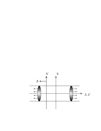
Figure 19: One dimensional expansion in a tube. The lab frame is labeled by $X$, $Y$, and $Z$, the boosted frame by $X^{\prime}$, $Y^{\prime}$, and $Z^{\prime}$ which is moving with a velocity of $\beta$ relative to the lab frame.

To study the frame dependence we will simulate the expansion in a so-called lab frame, whose origin agrees with the center of the expanding system and in a boosted reference frame, which is moving relatively to the lab frame with velocity $\beta=-\tanh\eta_{0}$. The situation is illustrated in Fig. 19. In the simulations we set $\eta_{0}=2$. Since particles are initialized longitudinally within a limited spatial region in rapidity, the pictures of the expansion in the two frames will be quite different. The expansion in the lab frame is symmetric, while in the boosted frame the right part of the system expands faster than the left part at late times. Therefore the expansion itself is frame dependent at late times due to the limitation of the particle initialization. We will concentrate on a so-called central region which is a cylinder around $\eta=0$ in the lab frame and correspondingly around $\eta_{0}$ in the boosted frame with a size of $\Delta\eta=1$. The time evolutions of observables such as $n(\tau)$, $\epsilon(\tau)$, $T(\tau)$, and others will be extracted in this central region in the two frames and will be compared. We will present the results in Sec. V.3.

Particles are initialized in the lab frame. At first we sample $\eta$ by its uniform distribution within $\eta\in[-3:3]$ at the starting time $\tau_{0}$. We then obtain the time and longitudinal position of the particle

$$t_{0}=\tau_{0}\cosh\eta,\quad z_{0}=\tau_{0}\sinh\eta\,.$$ (51)

The transverse positions $x_{0}$ and $y_{0}$ are sampled uniformly within the tube. Finally we determine the initial momentum according to the thermal distribution (41) at $\tau_{0}$ for given $\eta$. The initial positions and momenta of particles in the boosted frame are obtained by Lorentz transformations from the lab frame.

V.2 Improved cell configuration

Before we concentrate on the further analysis, we have to make sure that the cell configuration constructed in the last section is really suitable for an expanding system simulated by employing the stochastic method. To demonstrate this we perform a one dimensional expansion in the lab frame with the parameters set in the last section and extract $dN/d\eta$ distribution at time $t$. One expects that the distribution will be constant over a large region, since this was the basis motivation for the cell construction. Figure 20 shows the $dN/d\eta$ distribution within an interval of $\eta\in[-0.3:0.3]$ at time $0.11$, $0.13$, $0.16$ and $0.2$ fm/c. The dotted line depicts the initial value $dN/d\eta(\tau_{0})=1748$. Astonishingly, at first sight one notices a clear structure in the distribution within the $\eta$ bins. (Remember that the size of the $\eta$ bins is set to be $\Delta\eta_{c}=0.2$.) One can also realize that this structure approaches a characteristic final shape at late times. The meaning of the structure is that particles in a cell are spatially centered. This has no physical reason, but comes from a numerical artifact due to the finite size of the cell structure, which can be understood as follows: We concentrate on the central $\eta$ bin, $\eta\in[-0.1:0.1]$, and assume that the expanding system is in local thermal equilibrium. Any change of the $dN/d\eta$ distribution in the central $\eta$ bin is caused from collisions among the particles and from the ongoing particle diffusion. Even in the central $\eta$ bin the collective motion is still outwards in spite of the small flow velocity. There are more particles moving outwards than particles moving towards the center. Suppose two extreme cases of collision occurring in the central $\eta$ bin: In case 1 two particles are moving towards the center and are approaching each other. In case 2 two particles are moving outwards and back-to-back. Due to the considered isotropic scattering the momentum distribution of the particles after the collision is same in both cases. Since, on average, the case 2 happens more frequently than the case 1, one can draw the conclusion that collisions in an $\eta$ bin tend to bring more particles back into the center than to push them towards the outside when the collective flow in an $\eta$ bin is indeed directed outwards. This is the reason for the artificial structure of the $dN/d\eta$ distribution in the small $\eta$ bins. On the other hand, since the distribution of $dN/d\eta$ is no more constant, the particle diffusion from the center outwards is now stronger than the diffusion towards the center. The diffusion is thus counterbalancing the particle centralization and the $dN/d\eta$ distribution will approach a final shape when the balance between the diffusion and the centralization is fully established.

In Fig. 21 we compare the $dN/d\eta$ distributions at time $t=0.2$ fm/c from the simulations with $\Delta\eta_{c}=0.2$ and with a smaller size of $\Delta\eta_{c}=0.1$. In the simulation with $\Delta\eta_{c}=0.1$ we employ $2$ test particles per real particle in order to obtain the same statistics as in the case with $\Delta\eta_{c}=0.2$ and $N_{test}=1$. We see a weaking in the structure of $dN/d\eta$, though the structure does still exist. In the limit $\Delta\eta_{c}\to 0$, however, the characteristic substructure in the $dN/d\eta$ distribution will vanish, since the velocity of the intrinsic collective flow in the $\eta$ bins goes to zero. Therefore decreasing the size of the $\eta$ bins and using more test particles would be a natural way to reduce this numerical artifact. However, the more test particles, the longer will the computing time be. A more elaborate way which does not need further test particles is to move the cell configuration randomly from time to time. For instance, we move the central $\eta$ bin $\eta\in[-0.1:0.1]$ to $[-0.1+\xi:0.1+\xi]$, where $\xi$ is a random number distributed within $[0:\Delta\eta_{c}=0.2]$. Although particles in each $\eta$ bin will be still centered within each time step after collisions, but because of the random shift of the cell configuration the associated center of the bin for a particular particle is also moving, so that there is no absolute center for the particle. Therefore, on average, the effect of the centralization will be washed out. In Fig. 21 we depict the $dN/d\eta$ distribution from simulations employing the improved moving cell configuration with $\Delta\eta_{c}=0.2$. We see that the distribution is nearly constant and does not show any unwanted substructure. In Fig. 21 we also notice a tiny enhancement of the $dN/d\eta$ distribution when compared with the initial distribution $dN/d\eta=1748$. We will come back to this further artifact in the next subsection.

V.3 Results

V.3.1 $2\leftrightarrow 2$ processes without test particles

At first we present the results from simulations without test particles. Figures 22 and 23 show the time evolution of the particle density, energy density and temperature in the central space-time rapidity region in the two frames. The results are extracted from the simulations employing the geometrical and stochastic method respectively and are obtained by averaging $20$ independent realizations. The effective temperature is defined as $T=\epsilon/3n$ and corresponds to the statistical temperature when the system is at local kinetic equilibrium. Otherwise $T$ can be regarded as the mean energy per particle. In the simulation with the stochastic method we set the size of the $\eta$ bins to be $\Delta\eta_{c}=0.2$. The time scale in Figs. 22 and 23 denotes the time in the local frame of the central region. The solid and dotted curves depict the results achieved in the lab and boosted frame respectively. The thin solid lines show the ideal hydrodynamical limit calculated via a corresponding integral of the thermal phase space distribution (41). Please note that we have taken the size of the central region into account. Therefore the hydrodynamical results (43), (44), and (45) are modified by

$$n(t) = a_{n}\,n(\tau=t)\,,\quad a_{n}:=\frac{\Delta\eta}{2\,\tanh(\Delta\eta/2)}$$ (52)

$$\epsilon(t) = a_{\epsilon}\,\epsilon(\tau=t)\,,\quad a_{\epsilon}:=\frac{1}{6\,\tanh(\Delta\eta/2)}\,\int_{-\Delta\eta/2}^{\Delta\eta/2}d\eta^{\prime}\,\left(3+(\tanh\eta^{\prime})^{2}\right)(\cosh\eta^{\prime})^{4/3}$$ (53)

$$T(t) = a_{T}\,T(\tau=t)\,,\quad a_{T}:=\frac{a_{\epsilon}}{a_{n}}\,.$$ (54)

In the limit $\Delta\eta\to 0$ the additional factors go to $1$.

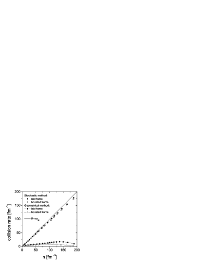
Figure 24: Collision rate in the central space-time rapidity region for various particle densities experienced during the expansion. The results are extracted from the same simulations performed for the extractions of $n(t)$ and $\epsilon(t)$ in Figs. 22 and 23. The solid line shows the analytical expectation.

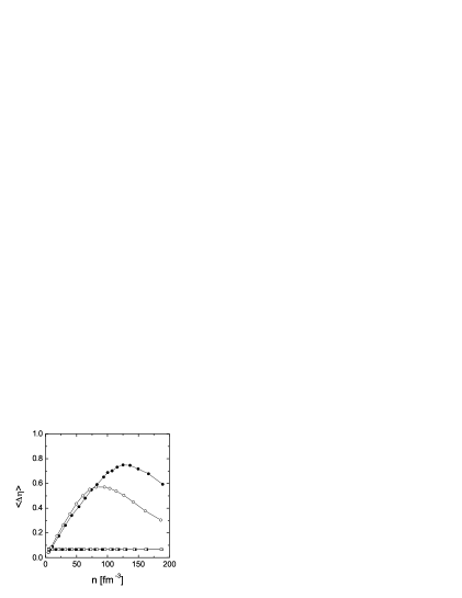
Figure 25: Averaged difference in space-time rapidity of colliding particles extracted in the central space-time rapidity region for various particle densities experienced during the expansion. The results are extracted from the same simulations performed for the extractions of $n(t)$ and $\epsilon(t)$ in Figs. 22 and 23. The labeling of the symbols is identical to that of Fig. 24.

From Figs. 22 and 23 we see that the frame dependence of the considered quantities is quite noticeable in the simulation when employing the geometrical method, while it is rather weak in the simulation employing the stochastic method. Moreover and astonishingly, the “temperature” in the simulation with the geometrical method is increased at the beginning of the expansion. This “reheating” [37] is unphysical, since the isotropic initialization of the particle system does not give any reason for an introversive pressure. The gradient of the pressure is directed outward, so that in the further evolution the longitudinal work done by the pressure should lead to a cooling of the system. We also rule out any explanation based on a possible viscous effect which might bring some effective net energy flow into the local region, because there is no reheating in the simulation with the stochastic method. From the investigations within a static box we have realized that the collision rate obtained in the simulation with the geometrical method will be suppressed when the mean free path is in the same order as (or even smaller than) the interaction length. This is indeed the situation at the beginning of the expansion in the tube. The suppression of collisions will obviously slow down the cooling of the system, but this cannot lead to any reheating. However, the fact that particles can interact with each other over a larger distance than the mean free path makes it reasonable that the pressure could be incorrectly built up. The effect of the “anti-pressure” is thus a numerical artifact. We extract the collision rate and the difference of space-time rapidities of colliding particles per collision event $<\Delta\eta>_{coll}$ in the central region from the simulations carried out in the lab and boosted frame. The results are depicted in Figs. 24 and 25. The collision rates are obtained by counting the collision events in the central region within a time interval of $0.02$ fm/c. It is clearly seen that the collision rates in the simulation with the stochastic method agree well with the expectation. The slight discrepancy can be understood as the consequence of the relative large size of the $\eta$ bins ($\Delta\eta_{c}=0.2$). In contrast, the collision rates in the simulation with the geometrical method are strongly suppressed at high densities due to the relativistic effect of the time spread of the two collision times, as explained in Sec. II.1. The results of the $<\Delta\eta>_{coll}$ show that particles interact in fact over very large distance at high densities in the simulation when employing the geometrical method. The decrease of the $<\Delta\eta>_{coll}$ at the highest densities corresponding to the very beginning of the expansion is due to the fact that at the early times particles with large $\eta$ are still not formed. In the simulation employing the stochastic method the interaction length is, however, controlled by the cell structure. In summary, we suspect that the larger interaction distance (compared with the mean free path) may be the reason for the “reheating”.

Figure 26 shows the space-time rapidity distributions at the proper time $\tau=0.2$ and $1.0$ fm/c extracted from the simulations in the lab and boosted frame with the geometrical (upper panel) and the stochastic (lower panel) method respectively. The solid (dotted) curves depict the distributions in the lab (boosted) frame. The thin solid lines show the initial distribution $dN/d\eta(\tau_{0})=1748$ within $\eta\in[-3:3]$. We see that the results obtained when employing the geometrical method show a strong frame dependence. A clear hump exists around the expansion center $\eta=0$ in both frames and broadens gradually. (Note that the expansion center in the boosted frame is at $\eta=-2$ after the shift.) The humps indicate a net particle diffusion towards the expansion center, which again can be explained as a consequence of the “antipressure” effect: The introversive pressure drives the particles back to the expansion center. In the distributions obtained when using the stochastic method we see a relative tiny hump at the expansion center which disappears at the later time. The slight enhancement has been also noticed in Fig. 21. We recognize that the size of the cell bins $\Delta\eta_{c}=0.2$ is not small enough to overcome the numerical artifact completely.

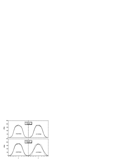
Figure 27: Particle distributions versus momentum rapidity at the proper time $\tau=0.2$ and $1.0$ fm/c extracted from simulations employing the geometrical and stochastic method in the lab and boosted frame. The results are obtained from the same simulations performed for the extractions of $dN/d\eta(\tau)$ in Fig. 26. The thin solid curves indicate the initial distribution at $\tau_{0}=0.1$ fm/c.

In Fig. 27 we depict the momentum rapidity distributions at proper times. The thin solid curves show the initial rapidity distribution

$$\frac{dN}{dy}(\tau_{0})=\frac{R^{2}T_{0}^{3}\tau_{0}}{\pi}\frac{\sinh(2\eta_{m})}{\cosh(2\eta_{m})+\cosh(2y)}\,,$$ (55)

where $\eta_{m}$ denotes the boundary of the initial system which has been set to be $3$. In the upper panel of Fig. 27 one also recognizes the particle diffusion towards the expansion center, though the effect is not strong. The disributions obtained when using the stochastic method show perfect “no frame dependence” and a collective flow outwards to the higher rapidity at late times.

For an initially thermal system it seems reasonable that the system will be still locally in or close to kinetic equilibrium during the further expansion. On the other hand, we have also realized that numerical artifacts make strong effects at the beginning of the expansion, especially in the simulations applying the geometrical algorithm. Therefore it is essential to question whether the encountered numerical problem does affect the maintenance of the kinetic equilibrium in the cascade simulations of the one dimensional expansion. For this we extract the transverse momentum distributions at $y=0$ within an interval $y\in[-0.5:0.5]$ at different proper times and compare them with the analytical thermal distributions. In Figs. 28 and 29 the $p_{T}$ distributions extracted from the simulations in the lab frame are depicted. Figure 28 shows the results at $\tau=1.0$ and $4.0$ fm/c in the simulations with the geometrical method and Fig. 29 shows the results at $\tau=0.2$, $1.0$ and $4.0$ fm/c in the simulations with the stochastic method. The thermal distributions shown by the solid lines are obtained as integral of the thermal particle distribution function (41) by means of the Cooper-Frye formula

$$\left.\frac{1}{N}\frac{dN}{p_{T}\,dp_{T}\,\Delta y}\right|_{y=0}(\tau)=\frac{1}{N}\frac{2\,\pi^{2}R^{2}}{(2\pi)^{3}}\frac{1}{\Delta y}\int_{-3}^{3}d\eta\int_{-\Delta y/2}^{\Delta y/2}dy\,p_{T}\,\tau\cosh(y-\eta)\,e^{-\frac{p_{T}\,\cosh(y-\eta)}{T(\tau)}}\,,$$ (56)

where $\Delta y=1$ and the temperature $T(\tau)$ is read off from Fig. 22 or Fig. 23 at $t=\tau$. We see good agreements between the numerical and the analytical distributions, even for the case of the geometrical method. The analogous $p_{T}$ distributions, extracted from the simulations in the boosted frame (at $y=\eta_{0}=2$), are also compared with the analytical spectra (both not shown in figures). The agreements are perfect as those presented in Figs. 28 and 29. As a conclusion, although the expansion does not proceed fully close to ideal hydrodynamics, the expanding system is still kinetically equilibrated at least until $\tau=4$ fm/c in the simulations with the stochastic method as well as with the geometrical method, although in the latter case the cooling of the system occurs much slower.

As a last point, we show in Fig. 30 the proper time evolution of the transverse energy extracted at $y=0$ per unit rapidity from both type of simulations in the lab and boosted frame respectively. The thin solid line depicts the result in the hydrodynamical limit

$$\left.\frac{dE_{T}}{dy}\right|_{y=0}(\tau) = \frac{\pi R^{2}}{(2\pi)^{3}}\int d\eta\,d^{2}p_{T}\,p_{T}^{2}\,\tau\cosh(y-\eta)\,e^{-\frac{p_{T}\,\cosh(y-\eta)}{T(\tau)}}$$ (57)

$$= \frac{3}{4}R^{2}\,T^{4}\,\tau=\frac{3}{4}R^{2}\,T_{0}^{4}\,\tau_{0}^{4/3}\,\tau^{-1/3}\,.$$

The time evolutions of the transverse energy have similar shapes like that of the temperature shown in Figs. 22 and 23. We also recognize the unphysical “reheating” occurring in the simulations with the standard geometrical method.

Summarizing this section, we have studied the frame dependence of a one dimensional expansion in a tube by employing the two collision algorithms presented in this paper. The comparisons show that quantities extracted in the simulations with the geometrical method have a much pronounced and unphysical frame dependence. Numerical artifacts are very significant in these simulations, especially at the beginning of the expansion when the system is very dense. In contrast, the results obtained from the simulations when employing the stochastic method show almost “no frame dependence”.

V.3.2 $2\leftrightarrow 2$ processes with test particles

The time evolutions of the particle density, energy density and temperature depicted in Figs. 22 and 23 demonstrate that simulated dynamics does not undergo an ideal hydrodynamical expansion. On the one hand, it is true that the ideal hydrodynamics cannot be realized in simulations with finite collision rate. One has to take the finite viscosity into account. Thus it is interesting to make comparisons between the transport results and those calculated from viscous hydrodynamics [57, 58, 59]. This subject is, however, beyond the scope of this paper. On the other hand, even the viscous expansion cannot be solved exactly due to the limitation of the numerical implementations. Especially, as observed in the simulations with the geometrical method, the numerical artifacts make strong unphysical effects. In this section we introduce the test particle method into the dynamics to reduce this numerical uncertainty and to study the convergency of the transport solutions.

From the experiences in the box calculations, one realizes that the computing becomes more time consuming when more and more test particles are added into the simulations. One way to reduce the computing time in the present case is to consider a tube with a smaller radius. The (real) particle density is however unchanged. In simulations with the geometrical method we set the radius of the tube to be $R^{\prime}=R/\sqrt{N_{test}}$ with $R=5$ fm. However, in simulations with the stochastic method we instead keep the radius of $5$ fm, in order to be able to refine the cell configuration.

Figure 31 depicts the relative frame dependence of the particle density, energy density, and temperature extracted in the central region in the simulations with the geometrical method with $N_{test}=1$, $4$, and $25$, respectively. The simulations are performed in the lab frame. We obtain the results by averaging $20$, $2$, and $20$ independent realizations, respectively. Note that the simulation with $N_{test}=4$ is exceptionally carried out with the default radius of $R=5$ fm. We see that the potential frame dependence is more and more reduced when more and more test particles are considered. The reduction of the frame dependence is also clearly demonstrated in Fig. 32. Here the distribution of the space-time rapidity obtained with $N_{test}=25$ is compared with the distribution without test particles (or $N_{test}=1$) at $\tau=0.2$ fm/c. The hump, which exists in the distribution without test particles due to the artificial back diffusion, does not occur with $N_{test}=25$. For the case employing the stochastic method it is not necessary to study the reduction of the frame dependence with the test particle method, since the frame dependence is actually very weak even without test particles (see Fig. 23).

We also employ the test particle method to study the convergency of the transport solutions. Figure 33 shows the time evolution of the temperature extracted in the central region in the simulations with increasing test particles in the lab frame. The size of the $\eta$ bins constructed in the simulations with the stochastic method is refined to $\Delta\eta_{c}=0.2/N_{test}$. There are on average $11$ test particles in one cell. (We have also performed simulations with doubled test particle number in one cell to increase the statistics. The outcome shows almost no changes.) From Fig. 33 we see the clear tendency of convergency. The time evolution of the temperatures extracted from the simulations with the geometrical and stochastic method converge towards almost the same curve. However, it is obvious that the solution obtained with the stochastic method converges more efficiently than the solution obtained with the geometrical method. Therefore, we do favour the stochastic method to be applied in transport simulations of system with high particle density. Furthermore, we see that the effect of the artificial reheating, appearing in the simulation with the geometrical method with $N_{test}=1$, reduces and vanishes in the simulations when employing higher test particles.

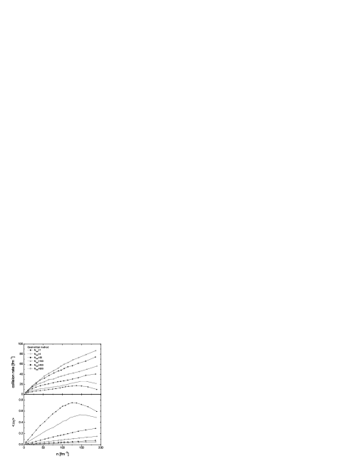
Figure 34: Collision rate and averaged difference in space-time rapidity of colliding particles. The results are extracted in the central space-time rapidity region $\eta\in[-0.5:0.5]$ for various particle densities experienced during the expansion. The simulations are the same as performed in the upper panel of Fig. 33 when discussing the convergency of the temperature.

In Fig. 34 we depict the collision rate and the mean difference of the space-time rapidities of colliding particles per collision $<\Delta\eta>_{coll}$ in the simulations with the geometrical method with increasing test particles. We see that the collision rate increases when using more test particles. However, even for $N_{test}=900$ the collision rates at high densities are still suppressed. The reason is that the interaction length decreases only with $1/\sqrt{N_{test}}$. We also see that the $<\Delta\eta>_{coll}$ decreases when the number of the test particles increases. Putting Fig. 34 in relation to Fig. 33 confirms our suspicion in the last subsection that unwanted collisions over large distances may lead to the buildup of “antipressure” which then influences the particle diffusion. We mention that the same numerical artifact has been found in the studies in Refs. [24, 37].

V.3.3 Including $2\leftrightarrow 3$ processes

We now include the inelastic $2\leftrightarrow 3$ processes into the dynamics of the one dimensional expansion in the tube and study the frame dependence for the new situation. The stochastic method is applied to simulate the (in)elastic collisions whose cross sections are set to be $\sigma_{22}=5$ mb and $\sigma_{23}=2.5$ mb. These parameters lead to the same rate of the elastic and inelastic transitions. We consider isotropic collisions and set the size of the $\eta$ bins to be $\Delta\eta_{c}=0.2/N_{test}$.

In Fig. 35 we show the time evolutions of the particle density, energy density, and temperature extracted in the central space-time rapidity region from the simulations with $N_{test}=1$ carried out in the lab and boosted frame. The results are absolutely frame independent. Comparing to the results with only two-body collisions shown in Fig. 23, we notice that the particle density is slightly enhanced. This enhancement is not due to any numerical artifacts, but the consequence of the chemical equilibration: In the thermal equilibrium the particle density is related with the temperature by $n=T^{3}/\pi^{2}$. Since during the expansion the temperature is always higher compared to the ideal hydrodynamical limit due to finite viscosity, therefore, there have to be more particles being produced than annihilated in order to account for the undersaturated system and to achieve a new balance. To address the chemical equilibration we concentrate on the time evolution of the fugacity which is defined as $\lambda(t)=n(t)/n^{eq}(t)$, where

$$n^{eq}(t)=a_{n}\,n^{eq}(\tau)=a_{n}\,\frac{T^{3}(\tau)}{\pi^{2}}=\frac{a_{n}}{a_{T}^{3}}\,\frac{T^{3}(t)}{\pi^{2}}\,.$$ (58)

$a_{n}$ and $a_{T}$ are factors given in Eqs. (52) and (54) taking the size of the central region into account. The $T(t)$ in Eq. (58) is just the extracted temperature from the simulation. Figure 36 depicts the time evolution of the fugacity. We see that the chemical equilibrium is almost achieved and maintained during the expansion in both frames. We have also extracted the $p_{T}$ distributions and compared with the analytical spectra at different times. The results show that the kinetic equilibrium is also maintained during the expansion.

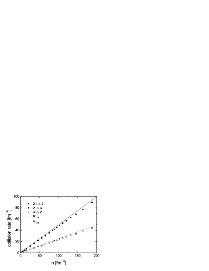
Figure 37: Collision rate in the central region for various particle densities experienced during the expansion. The results are extracted from the same simulations performed for the extractions of $n(t)$ and $\epsilon(t)$ in the lab frame in Fig. 35. The solid squares, solid circles and open circles depict, respectively, the collision rates for $2\leftrightarrow 2$, $2\to 3$, and $3\to 2$ transitions. The solid and dotted line show the analytical expectations.

The collision rates of $2\leftrightarrow 2$, $2\to 3$, and $3\to 2$ processes, extracted from the simulation in the lab frame, are depicted in Fig. 37. We see perfect agreements of the extracted collision rates with the expectations. Furthermore, the collision rates of $2\to 3$ and $3\to 2$ processes are almost identical, which demonstrates once more the maintenance of the chemical equilibrium in the expanding system.

We show in Fig. 38 the particle distributions versus the space-time rapidity $\eta$ and versus the momentum rapidity $y$ at $\tau=0.2$ and $1.0$ fm/c, obtained from the simulations with $N_{test}=1$ in the lab and boosted frame. The frame dependence is not noticeable and lies within the statistical errors. In Fig. 38 we also see the enhancement in the particle number over a large range due to the slight particle production in the ongoing chemical equilibration.

Finally, though the results from the simulations above are largely frame independent, convergence to the correct Boltzmann solutions requires using more test particles. Due to the settings of $\sigma_{22}=5$ mb and $\sigma_{23}=2.5$ mb one would expect that the total collision rate including elastic and inelastic processes is the same as that in the simulation with purely elastic collisions and $\sigma_{22}=10$ mb. Therefore, the convergence with increasing test particles would be exactly the same in both cases. Still, as realized from the above comparison between Figs. 35 and 23, the temperatures (and the number densities as well) in the central space-time rapidity region are slightly different due to the new balancing as explained above. Therefore, the convergence of the temperature, for instance, will not be the same as that shown in the lower panel of Fig. 33. On the other hand, the new balancing should not affect the time evolution of the energy density. (This quantity is shown in Fig. 39 for the pure $2\leftrightarrow 2$ and the $2\leftrightarrow 2$ + $2\leftrightarrow 3$ case with increasing $N_{test}$.) We see the exactly same convergence of the energy density in the central region.

After this exhaustive discussion of testing the operation of the cascade, we now proceed to describe real heavy ion collisions.

VI Full $3+1$ dimensional operation of the parton cascade for central Au+Au collisions at RHIC: kinetic and chemical equilibration

In this section we take the step to simulate the space time evolution of partons produced in a central Au+Au collision at maximal RHIC energy $\sqrt{s}=200$ GeV by means of the well-tested stochastic collision algorithm. The simulation is performed in the center-of-mass frame of the colliding nuclei. For the present and first exploratory study we include only the pQCD motivated gluonic interactions $gg\leftrightarrow gg$ and $gg\leftrightarrow ggg$ in the dynamical evolution. Simulations with all parton degrees of freedom will be postponed to a sequent paper.

VI.1 The initial conditions

The initial conditions for the parton cascade are assumed to be generated by minijet production in a central Au+Au collision modeled via multiple, binary nucleon-nucleon collisions [43, 44]. Of course, this is a strong assumption. The picture of the very early stage of the collision, when potentialy the partons are freed from the two nuclear wave functions and do become on-shell particles, is crucial for all kinetic cascades which can only describe the further evolution. Hence, one has to incorporate a physical model for describing the very initial phase of liberated partons serving as initial condition for cascades. One such physical picture is based on the idea of a free superposition of minijets being produced in the individual semihard nucleon-nucleon interactions. Another and much celebrated picture is the so-called McLerran-Venugopalan model or color glass condensate [45], which is based on the idea of gluon saturation of the QCD structure function of the nuclei at sufficiently low $x$. The so-called bottom up scenario [30] of thermalization relies on these initial conditions, where in the leading order of the coupling constant $\alpha_{s}$ the various time scales of kinetic evolution is parametrically estimated. We will leave this as an important task for future investigation. At present, we choose the liberation of minijets as the initial conditions. Minijets denote the on-shell partons with transverse momentum being larger than a centain cutoff value of $p_{0}\sim 2$ GeV. Since no nuclear effects like shadowing at small $x$ are considered in the present study, the averaged number of produced partons is then just proportional to the number of binary nucleon-nucleon collisions

$$<N_{parton}>\,=\,2\,\sigma_{jet}\,T_{AA}(b=0)\,.$$ (59)

$T_{AA}(b=0)$ denotes the nuclear overlap function for a central nucleus-nucleus collision. The overlap function is given by

$$T_{AB}({\bf b})=\int d^{2}x_{T1}dz_{1}\,d^{2}x_{T2}dz_{2}\,\,n_{A}({\bf r}_{1})\,n_{B}({\bf r}_{2})\,\delta^{2}({\bf b}-({\bf x}_{T1}-{\bf x}_{T2}))\,.$$ (60)

$n_{A/B}({\bf r})$ is the nuclear density. In physical terms, $\sigma T_{AB}(b)$, where $\sigma$ denotes the total nucleon-nucleon cross section, gives roughly the number of binary semihard nucleon-nucleon collisions in a $A+B$ collision at impact parameter $b$ [44]. The total jet cross section $\sigma_{jet}$ in a nucleon-nucleon collision at $\sqrt{s}=200$ GeV is calculated by integrating the differential jet cross section (28). The factor $2$ in Eq. (59) indicates that minijets are produced in pair. Employing the Woods-Saxon distribution for the nuclear density of a Lorentz contracted nucleus

$$n_{A}({\bf x}_{T1},z_{1})=\frac{\gamma\,n_{0}}{1+Exp\left((\sqrt{x^{2}_{T1}+(\gamma z_{1})^{2}}-R_{A})/d\right)}\,,$$ (61)

where $d=0.54$ fm, $R_{A}=1.12A^{1/3}-0.86A^{-1/3}$ fm, and $n_{0}$ is determined from the normalization $\int d^{3}r_{1}\,n_{A}=A$, one estimates that with a cutoff $p_{0}=2$ GeV about $1200$ minijets will be produced in a central Au+Au collision at maximal RHIC energy, in which $70\%$ are gluons. We note that this number does crucially depend on the cutoff $p_{0}$, which makes the minijet picture not so much promising. On the other hand, one might improve this by choosing some self-consistent relation for this crucial parameter [60].

The initializations of the individual produced partons in space-time and in momentum space are then realized statistically as follows: The momenta are sampled according to the differential jet cross section (28). This sampling has already been performed in Sec. IV when the thermalization of a parton system was studied within a fixed box. The space-time coordinates of the partons are obtained by a simple geometrical picture when the two Lorentz contracted nuclei do overlap. For convenience for the moment, we set the zero point of the time scale to be the moment of the full overlap. Then the longitudinal positions of the two nucleus centers are then at $\pm\,v\,t$, respectively, where $v$ is the velocity of the nuclei. One now identifies the intrinsic coordinates $z_{1}$ and $z_{2}$ in Eq. (60) with the global space and time coordinate

$$z_{1}=z-v\,t\qquad\mbox{and}\qquad z_{2}=z+v\,t\,.$$ (62)

Changing from $z_{1}$ and $z_{2}$ to $z$ and $t$ yields for Eq. (60) for $b=0$ and $A=B$

$$T_{AA}({\bf b}=0) = \int d^{2}x_{T1}\,d^{2}x_{T2}\,2\,v\,dt\,dz\,\,n_{A}({\bf x}_{T1},z-v\,t)\,n_{A}({\bf x}_{T2},z+v\,t)\,\delta^{2}({\bf x}_{T1}-{\bf x}_{T2})$$ (63)

$$= \int d^{2}x_{T1}\,2\,v\,dt\,dz\,\,n_{A}({\bf x}_{T1},z-v\,t)\,n_{A}({\bf x}_{T1},z+v\,t)\,.$$

One thus receives the statistical distribution for sampling the space-time coordinates of the individual produced partons

$$\frac{d<N_{parton}>}{d^{2}x_{T1}\,dz\,dt}\sim n_{A}({\bf x}_{T1},z-v\,t)\,n_{A}({\bf x}_{T1},z+v\,t)\,.$$ (64)

The probability for producing a parton at $({\bf r},t)$ is thus proportional to the convolution of the nuclear densities of the two overlapping nuclei at the individual space-time point. Due to the choice of the zero point in time, about half of the produced partons are liberated at negative times. Therefore, with this convention of the zero point in time the space-time rapidity $\eta$ (42) is not a well-defined quantity. In order to correct this, we shift all the times to be larger than the absolute values of the corresponding longitudinal positions, i.e., $t\to t+t_{s}>|z|$, with a uniquely chosen $t_{s}$. This actually implies that $t_{s}\sim 0.5R_{A}/\gamma$, i.e., half of the overlapping time. Since we apply Woods-Saxon distribution (61) for the nuclear density, we cannot exactly specify when the first touch of the two colliding nuclei occurs. $t_{s}$ is thus - strictly speaking - a parameter in our simulation. For a larger $t_{s}$ particles pile up in the central space-time rapidity region and for a smaller $t_{s}$ particles distribute within a wider rapidity range during the very early evolution. On the other hand, independently on the chosen $t_{s}$, most of the partons are in fact produced in the central rapidity region due to the geometry of the overlapping nuclei. In the simulations we determine $t_{s}$ with the assumption that the initial partons are distributed within a space-time rapidity range of $\eta\in[-5:5]$.

In the above picture concerning the implementation of the space-time production of minijets, it is assumed that partons become immediately on-shell when the (semi)hard nucleon-nucleon collisions occur. Alternatively, one may introduce an additional formation time for every minijet, $\Delta t_{f}=\cosh y\,\Delta\tau_{f}\approx\cosh y\cdot 1/p_{T}$, which models the off-shell propagation of the freed partons. Within that time span, one assumes, for simplicity, that the still virtual parton does not interact and moves with speed of light. We realize, confirmed by numerical simulations, that the introduction of such a formation time does not affect our main findings too much. A further brief discussion will follow in Sec. VI.4. We note that the consideration of the initial conditions of partons is a reasonable description of the minijet production in space-time according to the overlapping of two heavy ions. These are different from the Bjorken-type initial conditions as considered in Refs. [24, 28]. Therefore, the initial correlation between the space-time and momentum rapidity, $\eta-y$ correlation, cannot be expected as the simple $\eta=y$. Detailed analysis will be shown in Sec. VI.4.

VI.2 Cell configuration

To be able to apply the stochastic method to simulate the full collision sequences, we divide the space into appropriate cells. The individual cell structure has to be considered selfconsistently to be well suited to the details of the dynamical evolution of the parton system. Since it is not clear whether the parton evolution is invariant under the Bjorken boost, a configuration with constant division in space-time rapidity, $\Delta\eta=$constant, as chosen in Sec. V when simulating one dimensional expansion of a thermal system in a tube, is here not really reliable. Cell structure should be refreshed every time step to adapt to the dynamical parton evolution. In principle, one dimensional expansion is still a good approximation for the whole parton evolution for the first few fm/c after a nucleus-nucleus collision. We thus still employ a static cell configuration in the transverse plan: Cells are transversely set as squares with a length of $0.5$ fm. Longitudinally, space is divided into $\Delta z$ bins, where each bin contains about the same number of test particles. This ensures the same statistics for each bin and automatically adapts to the density profile of the evolving parton system. This dynamical structuring begins at the center of the fire-ball and then proceeds to the very outside. Test particles from the far outside are not included into the cell configuration, because there the density distribution is too inhomogeneous. Instead, we then consider only elastic scatterings among these partons treated via the geometrical method. To obtain sufficient statistics, one has to tune the test particle number in each bin to be large enough: It turns out that a number of $20$ test particles on average in each cell is sufficient during first $4\sim 5$ fm/c. However, in the region with lower particle density, especially in the transversal surface, there are not enough test particles. If the test particle number in a cell is less than a certain cutoff, which is set to be $4$ in the simulations, we treat test particles in this cell again only by means of elastic scatterings with the geometrical method. How fine the longitudinal bins would be, depends on $N_{test}$, the number of test particles per real particle. We set $N_{test}=60$ in the simulations. In total, this leads to an equivalent division of roughly equally sized bins in space-time rapidity with $\Delta\eta=0.1\sim 0.2$. Furthermore, in order to avoid that particles belong to the same cell for too long time, as discussed in Sec. V, we randomly shift the cell structure by a small amount in the longitudinal as well as transversal direction after every time step.

Besides this fine mesh of cells we also have to choose a sufficiently small time step to prevent a too strong change of the spatial configuration in each local cell. In the simulations, this time step is time dependent and is determined to be the one-fifth of the smallest occurring cell length. For the case that a collision probability turns out to be greater than $1$, all operations done within the current time step are redone with an appropriately chosen smaller time step.

VI.3 Assumptions

We calculate the dynamical screening mass $m_{D}^{2}$ in a similar way as done for the box calculations in Sec. IV [20]

$$m_{D}^{2}=16\pi\alpha_{s}\int\frac{d^{3}p}{(2\pi)^{3}\,p}\,N_{c}\,f_{g}\approx 16\pi\alpha_{s}N_{c}\frac{1}{V}\sum_{i}\frac{1}{p_{i}}\,.$$ (65)

The evaluation is carried out (quasi)locally. $V$ denotes the volume of a local region and the sum runs over all test particles in the region. The presence of the cell structure makes it reasonable to calculate the screening mass in each cell. However, the statistical uncertainty due to fluctuations is still large, since there are at maximum $20\sim 30$ test particles in one individual cell, and thus an extraction of the particle phase space density $f$ is not precise. If one assumes that the expansion in the first few fm/c is mainly longitudinal, and further, that the transverse parton distribution is homogeneous over a large transversal area, one can extend the sum in Eq. (65) over a more broader region compared to the individual cell. In the simulations we consider a volume $V$ as a cylinder with a radius of $6$ fm in the individual $\Delta z$ bin. Within each bin $m_{D}^{2}/\alpha_{s}$ is assumed to be transversely constant. This approximation will lead to an underestimate of $m_{D}^{2}/\alpha_{s}$ in the very central area and an overestimate in the outside area when the transverse flow builds up, since within the same $\Delta z$ bin the particles moving with larger transverse velocity have larger energy and thus make a smaller contribution to the sum in Eq. (65) than the particles moving with smaller transverse velocity. The radius is a parameter which we set to be roughly equal to the radius of a Au nucleus. It turns out that the influence of this parameter on the screening mass is still quite sensitive at least for late times. A future improvement will be to simulate the parton evolution within a parallel ensemble technique, which will give the possibility to extract the particle phase space density locally more precise.

The coupling $\alpha_{s}$ is assumed to be

$$\alpha_{s}(Q^{2})=\alpha_{s}(s)=\frac{12\,\pi}{(33-2\,n_{f})\,\ln(s/\Lambda_{QCD}^{2})}$$ (66)

for individual collisions, where $s$ denotes the invariant mass of a particular colliding system of two or three particles. We set the quark flavour $n_{f}$ to be $3$ and $\Lambda_{QCD}$ to be $200$ MeV. In general, $Q^{2}$ in Eq. (66) stands for the momentum transfer in collision such as in deep inelastic scattering. For many-body collisions, however, the scale $Q^{2}$ is not unambiguous.

The gluon collision rate $R_{g}$, which will be employed to determine the effectively incorporated Landau-Pomeranchuk suppression in the $gg\leftrightarrow ggg$ processes by means of a low-momentum cutoff, is evaluated locally in cells

$$R_{g} = R_{gg\to gg}+R_{gg\to ggg}+R_{ggg\to gg}\,,$$

where

$$R_{gg\to f} = \frac{\sum_{i}P_{i}^{gg\to f}}{\frac{1}{2}N_{g}\Delta\tau}\,,\quad f=gg,ggg,\quad\mbox{and}$$ (67)

$$R_{ggg\to gg} = \frac{\sum_{i}P_{i}^{ggg\to gg}}{\frac{1}{2}N_{g}\Delta\tau}\,.$$ (68)

The $P_{i}$s denote the respective individual collision probabilities. The sum over $P_{i}$ gives the mean number of collisions occurring during a time step $\Delta t$ in a cell with $N_{g}$ gluons. $\Delta\tau$ denotes the corresponding time interval in the comoving frame $\Delta\tau=\Delta t/\gamma$, where $\gamma=1/\sqrt{1-v^{2}/c^{2}}$ and $v$ is the collective velocity of the moving cell. For a cell with about $20$ gluons there are totally $200$ individual possible $gg\to gg$ and $gg\to ggg$ collisions each and $1200$ possible $ggg\to gg$ collisions. The statistics is high enough to ensure evaluations of the collision rates in local cells to be sufficiently precise, in contrast to the calculation of the screening mass. Still a problem remains, which is that the calculation of the collision probability for a $ggg\to gg$ process by a two dimensional integral is time consuming. To reduce the computing time we have to take the following approximation, which has already been applied for the box calculations in Sec. IV: We randomly choose about $20$ gluon triplets instead of the total $1200$ combinations and compute the amplified collision probabilities (27). Therefore the statistical fluctuation of the collision rate $R_{ggg\to gg}$ is stronger than that of the others. Also, when extracting the velocity of an individual space element we encounter the same difficulty of insufficient statistics as explained by calculating the screening mass. We assume that all the cells in a $\Delta z$ bin have the same longitudinal velocity

$$v=\frac{V\,\int\frac{d^{3}p}{(2\pi)^{3}}\,\frac{p_{z}}{E}\,f}{V\,\int\frac{d^{3}p}{(2\pi)^{3}}\,f}\approx\frac{1}{N_{g}}\,\sum_{i}\frac{p_{iz}}{E_{i}}\,,$$ (69)

where the sum runs over the test particles within a cylinder with a radius of $6$ fm in the considered $\Delta z$ bin, and $N_{g}$ denotes the gluon number in the cylinder. The transverse component of the velocity is set to be zero. In principle, this assumption can be corrected when a parallel computing device is employed for achieving much higher statistics. Then one is able to look for and calculate transverse flow of each individual cell more accurately.

VI.4 Results

VI.4.1 Rapidity distributions

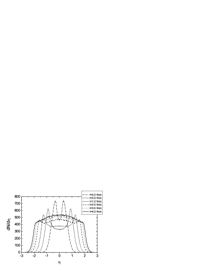
Figure 40: Gluon number distribution versus space-time rapidity at the time $t=0.2$, $0.5$, $1.0$, $2.0$, $3.0$, and $4.0$ fm/c during the expansion in a real, fully $3$D central Au+Au collision at the maximal RHIC energy.

We now present first numerical results obtained for the time evolution of the gluons produced in a central Au+Au collision at RHIC energy $\sqrt{s}=200$A GeV. In the simulations the number of the test particles is set to be $N_{test}=60$. All results are obtained by an average over $30$ independent realizations. Figures 40 and 41 show the particle number distributions per unit rapidity versus the space-time rapidity and the momentum rapidity at the times $0.2$, $0.5$, $1.0$, $2.0$, $3.0$, and $4.0$ fm/c, respectively. The time interval of the overlapping for the two Au nuclei is about $0.17$ fm/c. Therefore, the first extraction at $0.2$ fm/c is just after the end of the production of the primary partons (or minijets). In Fig. 40 one sees a noticeable spreading of the $dN/d\eta$ distribution with progressing time. The reason is that the initially produced partons are distributed within a very small longitudinal region due to the Lorentz contraction of the Au nuclei. Their momentum rapidities, however, have a wider distribution, as can be seen in Fig. 41. The spreading of the space-time rapidity distribution continues until its width reaches a comparable magnitude with that of the momentum rapidity distribution. For the special case of a simple noninteracting free streaming system, the $dN/d\eta$ distribution will then have exactly the same shape as the $dN/dy$ distribution at late times. In the present case we see that at $4$ fm/c the width of space-time rapidity distribution is about $4.2$ and approaches nearly the width of the distribution of the momentum rapidity being about $5$. It can be clearly seen that the spreading of the $dN/d\eta$ distribution indeed slows down at late times. In the central space-time rapidity region the gluon density first decreases due to this spreading, and then increases because of the ongoing gluon production via the $gg\to ggg$ process. The gluon multiplication is most clearly demonstrated by inspecting the momentum rapidity distributions in Fig. 41, where for instance at $y=0$ the gluon number is double amplified until $4$ fm/c. Moreover, at late times the net gluon production slows down, which implies the completion of the ongoing chemical equilibration. Of course, from the momentum rapidity distributions it is difficult to recognize any evidences for kinetic equilibrium. To investigate whether the system indeed does thermalize or not, one needs more detailed analyses in sufficiently local regions. We will present the results in next subsection.

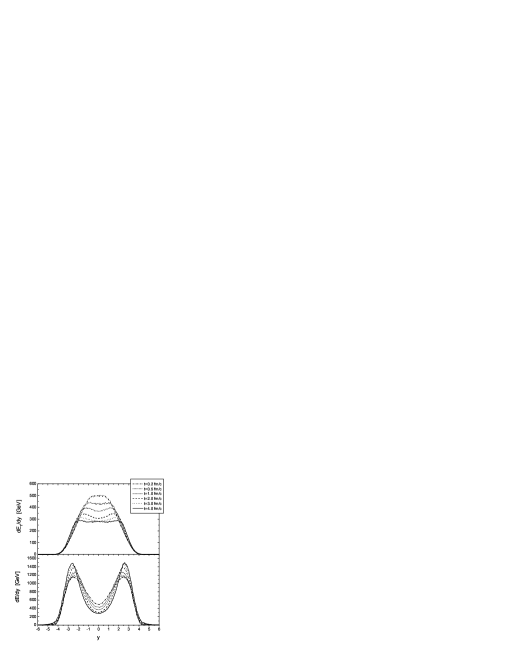
Figure 42: Momentum rapidity distributions of the transverse energy (upper panel) and the total energy (lower panel) of gluons at the time $t=0.2$, $0.5$, $1.0$, $2.0$, $3.0$, and $4.0$ fm/c during the expansion.

Figure 42 shows the momentum rapidity distributions of the transverse energy (upper panel) and the total energy (lower panel) at the different times during the expansion. While the distributions would not change during an evolution like free streaming, we see in Fig. 42 the decrease of the transverse energy and the energy transport from the center towards the higher rapidity due to the longitudinal work done by the pressure. This gives first significant indications of collective behavior. In addition, we note that when comparing Fig. 41 with the upper panel of Fig. 42, the shape of the latter clearly looks more alike one dimensional Bjorken expansion than that for the particle number distribution. Hence, one cannot really conclude that the simple Bjorken expansion of constant $dE_{T}/dy$ and $dN/dy$ manifests.

VI.4.2 Thermalization

In the following we study possible gluon thermalization in the “central region” being defined as a longitudinally expanding cylinder located in the middle of the expanding system. The radius of the cylinder is fixed to be $1.5$ fm and its length is $\Delta\eta=1.0$ from $-0.5$ to $0.5$. In view of the possible buildup of transverse flow, one could consider a cylinder with varying radius which is comparable with the longitudinal length. On the other hand, however, the statistics within such cylinder would be very low at early times. Since the analysis of transverse flow, which we want to address in a further paper, shows that the transverse flow velocity is not large close to the central region even at time of $4$ fm/c, the above choice with fixed radius is a reasonable compromise.

In Fig. 43 we depict the time evolution of the gluon density and energy density in the central region. The densities are very high at early times. Alternatively, an implementation of the formation time for gluons, as briefly outlined at the end of Sec. VI.1, strongly reduces the densities at early times: $n\sim 20$ $\mbox{fm}^{-3}$ and $\epsilon\sim 50$ $\mbox{GeV fm}^{-3}$ before $0.3$ fm/c. After that time the results for the particle and energy density with and without the formation time are nearly identical throughout the subsequent evolution. It shows that even if the densities are very high at very early times with no formation time, the gluons rather stream freely within the first $0.3-0.4$ fm/c. At $4$ fm/c the energy density is still $1$ $\mbox{GeV fm}^{-3}$. Thus the parton picture of particle interactions is valid for the first $4$ fm/c in a central Au+Au collision at RHIC. After that hadronization should occur and the system is then in a parton-hadron “mixed phase”.

Figure 44 shows the spectra of transverse momentum in the central region at different times during the expansion. The bold-folded histogram, which has a lower cutoff at $2$ GeV, depicts the initial distribution of the primary gluons (minijets). The spectrum possesses a typical power-law behavior. Already at $0.2$ to $0.5$ fm/c a tremendous population of the soft gluons below $2$ GeV has taken place. However, still a remedy of the edge at $2$ GeV in spectra is visible. The “edge” vanishes at about $1$ fm/c and the distributions become nearly exponential and progressingly steepen at the later times $2$, $3$, and $4$ fm/c. The ongoing steepening of the spectra in time represents a further strong indication of a (quasi)hydrodynamical expansion of an almost kinetically equilibrated system with decreasing temperature.

To study kinetic equilibration in more detail, we first concentrate on the momentum anisotropy $<p_{T}^{2}>/2<p_{z}^{2}>$. For an ideal, one dimensional boost-invariant hydrodynamical expansion the value of the anisotropy extracted within a region $\eta\in[-\Delta\eta/2,\Delta\eta/2]$ is given by

$$\frac{<p_{T}^{2}>}{2\,<p_{z}^{2}>} = \frac{\int_{-\tilde{z}}^{\tilde{z}}dz\int d^{2}p_{T}dy\,E\,p_{T}^{2}\,e^{-\frac{p_{\perp}\cosh(y-\eta)}{T(\tau)}}}{2\,\int_{-\tilde{z}}^{\tilde{z}}dz\int d^{2}p_{T}dy\,E\,p_{z}^{2}\,e^{-\frac{p_{\perp}\cosh(y-\eta)}{T(\tau)}}}$$ (70)

$$= \frac{\int_{0}^{\Delta\eta/2}d\eta\,(\cosh\eta)^{2/3}}{6\int_{0}^{\Delta\eta/2}d\eta\,(\cosh\eta)^{8/3}-5\int_{0}^{\Delta\eta/2}d\eta\,(\cosh\eta)^{2/3}}\,,$$

where $\tilde{z}=t\,\tanh(\Delta\eta/2)$. The expression (70) depends only on the longitudinal length of the local region where the momentum anisotropy is extracted, and goes to $1$ in the limit $\Delta\eta\to 0$. In the central region with $\Delta\eta=1$, the anisotropy is equal to $0.65$ for an ideal expansion. In Fig. 45 the time evolution of the momentum anisotropy extracted from the present simulations is depicted by the solid curve. Compared with the thermal value $(0.65)$, the curve in Fig. 45 shows first a significant increase during a short time $0.6$ fm/c and then a smooth relaxation to that thermal value. The early increase of the momentum anisotropy is due to the initial $p_{T}$ cutoff, $p_{T}>2$ GeV, and the fact that the primary gluons with large longitudinal momentum also have large rapidity and thus move rapidly out of the central space-time rapidity region. The following decrease of the anisotropy unambiguously implies the ongoing persistance of kinetic equilibration. The reason why the anisotropy is still larger than the thermal value is due to the fact that particles with larger $p_{T}$ equilibrate later, as also seen from the $p_{T}$ spectra in Fig. 44. From that particular analysis, quantitatively, the gluon system becomes approximately fully equilibrated at $2.5$ fm/c. On the other hand, as just stated, the clear bending over at a time of $0.75$ fm/c signals that the strong thermalization has already started at that time, as one also notices from the onset of the pronounced exponential behavior at a similar time as seen in Fig. 44.

The rapid streaming of the high-energy particles out of the central region at the beginning of the expansion also explains the dramatic decrease of the gluon density, energy density (both shown in Fig. 43) and the effective temperature $T=\epsilon/3n$ at early times, which is shown in the upper panel of Fig. 46 by the solid curve. The further decrease of the temperature until $200$ MeV at $4$ fm/c is due to the fact that work is done by the pressure and also due to the ongoing production of gluons. In case of simple free streaming the effective temperature would be constant over the whole time. To characterize the time dependence of the temperature we assume that the temperature behaves like $T\sim 1/t^{\alpha}$ with a time dependent exponent. $\alpha(t)$ is shown in the lower panel of Fig. 46. We see that the exponent is almost constant, about $0.6$, at late times and is roughly double the size of $1/3$, which one expects for an ideal, one dimensional boost-invariant expansion. This might indicate the buildup of transverse flow, but is mainly due to the further production of gluons. For this we also extract the gluon fugacity from the simulations and depict its time evolution in Fig. 47 in a way similar as in Sec. IV [see Eq. (38)]. Until $4$ fm/c the chemical equilibration is still not fully achieved. Inspecting again Fig. 43, we have also plotted there for comparison the standard Bjorken behavior $n\sim 1/t$ and $\epsilon\sim 1/t^{4/3}$ with a fixed intercept at time $t=0.5$ fm/c. One clearly recognizes that the particle number density decreases more slowly (with an exponent of about $-0.7$) due to the particle production. On the other hand, most interestingly, the energy density more or less exactly follows the form which one would expect from ideal Bjorken hydrodynamics. Indeed, the standard relation $P=\epsilon/3$ is all what enters into ideal hydrodynamical evolution for massless constituents, irrespective whether the system is chemically saturated or not. This finding gives another evidence that the system in the central region behaves nearly as an ideal fluid. We conclude that starting from the special, yet highly nonthermal initial condition a gluon plasma, even not fully thermalized, may form at $1$ fm/c in a central Au+Au collision at RHIC energy and its ongoing evolution in bulk behaves (quasi)hydrodynamically.

We have to note here that, of course, this reasoning will depend crucially on the initial conditions chosen. If we would only double the number of initial gluons, thermalization should roughly occur twice as fast. Indeed, our initial gluon number is lower compared to other studies in the literature [28, 60], where a factor of $2-4$ more initial gluons is assumed. This will then clearly imply that full gluon equilibration within a consistent pQCD approach can have a full realization at RHIC. A detailed study, addressing various initial conditions for the gluon number, i.e., different forms of minijet productions or color glass condensate initial conditions, has to and will be done in a further publication.

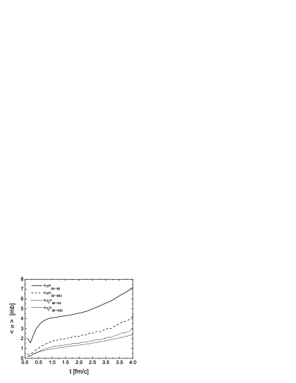
Figure 48: Time evolution of the averaged cross section and the averaged transport cross section in the central region. The solid and dashed (short-dashed and short-dotted) curves depict the averaged cross sections (transport cross sections) for the $gg\to gg$ and $gg\to ggg$ processes, respectively.

Figure 48 shows the time evolution of the cross sections which are first calculated as ensemble averages over all the possible collisions in a cell and then averaged over all the cells within the central region. As $<v_{rel}>\approx 1$ in the central region, the collision rates of the $gg\leftrightarrow gg$ and $gg\to ggg$ are obtained by $R=n<v_{rel}\sigma>\approx n<\sigma>$, respectively. We have compared these collision rates with those counted directly from the simulation and have seen nice agreements. The increase in time of the two cross sections is due to the fact that the cross sections are inversely proportional to the screening mass squared and the latter is proportional to the temperature squared. One sees that $\sigma_{gg\to gg}$ is always larger than $\sigma_{gg\to ggg}$. For kinetic equilibration, however, not only a large total cross section but also large scattering angle are essential for a possible fast thermalization. In other word, the transport cross section

$$\sigma_{t}=\int d\sigma\,\sin^{2}\theta_{c.m.}=\int d\theta_{c.m.}\,\frac{d\sigma}{d\theta_{c.m.}}\,\sin^{2}\theta_{c.m.}$$ (71)

is the key quantity controlling the ongoing of the equilibration by given particle density $n$. $\theta_{c.m.}$ denotes the scattering angle in the center of mass frame of the colliding particles. For a $gg\to ggg$ process each outgoing particle has its own scattering angle. In this case we modify Eq. (71) by $(\sin^{2}\theta_{1}+\sin^{2}\theta_{2}+\sin^{2}\theta_{3})/3$ instead of $\sin^{2}\theta_{c.m.}$. The averaged transport cross sections are shown in Fig. 48 by the short dashed and short dotted curves. Taking into account that at late times the collision rate of the $ggg\to gg$ is comparable with the rate of the $gg\to ggg$ process, one realizes that the inelastic processes are actually the dominant processes driving the system to kinetic equilibrium. The ensemble averaged running coupling $<\alpha_{s}>$ is also extracted within the central region during the gluon evolution. It turns out that $<\alpha_{s}>$ increases almost logarithmically in time from $0.2$ at $0.2$ fm/c to $0.5\sim 0.7$ at $4$ fm/c. We note that when comparing the cross sections calculated in thermal equilibrium (see Fig. 11), the cross sections $\sigma_{gg\to gg}$ and $\sigma_{gg\to ggg}$ extracted from the dynamical runs are $4\sim 5$ times larger at later times. This is because first $\alpha_{s}$ had been fixed to $0.3$ in Fig. 11 and is thus smaller. Second, the screening mass is appreciably smaller in the dynamical calculation as the gluons are not fully saturated in its occupation number. Both effects add up to the difference.

Following the expression of the differential cross section one knows that the gluon elastic collisions favor small angle scatterings. The transport cross sections in Fig. 48 indicate that the angular distribution of the inelastic collisions is more moderate than that of the elastic collisions. As can be realized from the differential cross sections expressed in Appendices C and D, the angular distribution of the elastic scatterings depends on $m_{D}^{2}/s$, while it depends on $m_{D}^{2}/s$ and $\lambda_{g}\sqrt{s}$ for the inelastic collisions. In Fig. 49 we depict the angular distributions of the $gg\to gg$ and $gg\to ggg$ scatterings for the parameters $m_{D}^{2}/s=0.05$ and $\lambda_{g}\sqrt{s}=4$. The distributions are calculated according to the differential cross sections. The two parameters are chosen from an intermediate situation within the simulation. We see that while the angular distribution of the elastic collisions clearly shows forward scatterings as expected, the angular distribution of the inelastic collisions is surprisingly almost isotropic. The reason for this behavior is due to the effective Landau-Pomeranchuk cutoff being implemented. For a larger $\lambda_{g}\sqrt{s}$ the $gg\leftrightarrow ggg$ processes would also favor the more the small angle scatterings. Notice that $\theta_{3}$ denotes the angle of the radiated gluon and thus possesses also a cutoff in its distribution due to the incorporation of the Landau-Pomeranchuk suppression of low momentum gluon emissions.

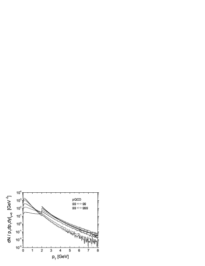
Figure 50: Transverse momentum spectrum in the central space-time rapidity slice ($\eta\in[-0.5:0.5]$ and all gluons in the transverse plan are counted for) at different times ($t=0.2$, $0.5$, $1.0$, $2.0$, $3.0$, and $4.0$ fm/c from second upper to lowest histogram). The most-upper and bold-folded histogram with a lower cutoff at $p_{T}=2$ GeV denotes the spectrum of the primary gluons (minijets).

In Fig. 50 we present the $p_{T}$ spectra at different times in the central momentum rapidity integrated now over the whole transverse region. The spectra are arranged in the same way as in Fig. 44. Comparing the spectra in Fig. 50 with those in Fig. 44, we see that there is no full global thermalization over whole transverse region until $4$ fm/c. At least for the lower momenta we see a nearly exponential population and a clear steepening at the later stages. Part of the minijet spectra, of course, survives as those gluons might escape directly from the outer region without interactions. In addition, Fig. 50 also demonstrates the potential energy loss of gluons due to the Bremsstrahlung process. The new developed parton cascade offers an alternative possibility to investigate the phenomenon of the jet quenching in a more quantitative way based on a full $3+1$ dimensional treatment of the geometry. To be able to compare the numerical results with the experimental data one has to model the mechanism of the hadronization and include further hadronic interactions. A detailed analysis is again one of possible future projects.

VI.4.3 Simulation only with elastic scatterings

In order to further focus on the importance of the inelastic channels to the evolution, to the thermalization and to the potential onset of nearly ideal hydrodynamical behavior of the partonic system, we now perform simulations, for comparison, only with pure elastic scatterings among the gluons. Since in this case no gluons will be produced during the evolution, more test particles are needed to build for a fine cell structure. We set $N_{test}=240$. Fig. 51 depicts the spectra of the transverse momentum in the central region at different times. The population of the soft gluons below $2$ GeV is rather low and the distributions at large $p_{T}$ are only slightly altered. Indeed gluons with highest momenta get more populated. It is obvious that the gluon system is not thermalized during the expansion. This can also be realized from the time evolution of the momentum anisotropy presented in Fig. 45 by the dashed curve, where the anisotropy saturates at much higher value than $1$ at late times. Furthermore, the constant temperature shown in Fig. 46 indicates that the evolution of the gluons is almost close to free streaming. (Please note that the abrupt decrease before $0.5$ fm/c is also due to the free streaming of the energetic gluons out of the central space-time rapidity region.) We remark that in the full dynamics with the inelastic channel, the contribution of the elastic scatterings to kinetic equilibration is actually significantly larger than that shown here, because in the full dynamics we have more gluons due to the radiation and the transport cross section also becomes larger compared to a nonequilibrated system.

In principle, kinetic equilibration can be achieved by elastic scatterings alone, if ad hoc the transport cross section is chosen sufficiently large. To demonstrate this we carry out simulations with isotropic collisions and a large and constant total cross section of $\sigma_{22}=30$ mb. The corresponding transport cross section is thus $20$ mb. Such extreme conditions of an assumed large opacity in $2\leftrightarrow 2$ reactions have been used in Ref. [28] to study the possible buildup of elliptic flow. Figure 52 shows the $p_{T}$ spectra in the central region at different times. Indeed we observe fast equilibration. The spectrum at $0.5$ fm/c is almost thermal. At the later times the distributions become more and more steeper, which indicates the cooling down of the system due to (quasi)hydrodynamical expansion. The time evolution of the momentum anisotropy, the dotted curve in Fig. 45, shows that from $1.0$ fm/c the anisotropy is almost constant and slightly higher than the value of the ideal, one dimensional boost-invariant expansion, $0.65$. Moreover, also the exponent describing the cooling of the temperature (see Fig. 46), $\alpha(t)$, is nearly constant from $1$ to $3$ fm/c and only slightly greater than the value of the ideal expansion, $1/3$. All this demonstrates that for the given extreme conditions the gluon system equilibrates indeed rapidly and then expands nearly hydrodynamically according to the ideal Bjorken scenario. However, of course, the constant and isotropic cross section cannot be further motivated. In addition, following that particular evolution, the system would stay for a rather long time in a hot, but very dilute and undersaturated (in its gluon number) deconfined state (see upper Fig. 46). Contrary, in the more realistic situation with inelastic collisions included, the temperature drops much more dramatically and the system would stay only until $t\approx 4$ fm/c in a pure deconfined state, being then (nearly) fully saturated in the gluonic degrees of freedom, and will then hadronize.

Figure 53 shows the time evolution of the transverse energy per unit momentum rapidity at midrapidity for the three cases compared also in Figs. 45 and 46. We see that the transverse energy decreases in the simulation including pQCD elastic and inelastic interactions and in the simulation employing an isotropic, large cross section. In contrast to the cooling of the temperature, to which the production of gluons also contributes, the decrease of the transverse energy within a unit rapidity is purely due to the longitudinal work done by the pressure! In the simulation employing large and constant cross section, energetic gluons are extremely stopped during their formation periode, so that the transverse energy is very large at very early times and pressure seems to be already built up during the overlap of two nuclei. This leads to the following (unrealistic) strong explosion with drastical cooling. The unaltered behavior of the transverse energy in the simulation including only pQCD elastic scatterings indicates again that in this case the parton evolution resembles a free streaming. One observes that from times $t\approx 0.5$ fm/c both the full pQCD (including $gg\leftrightarrow ggg$) and the “strongly coupled” (with isotropic $\sigma_{22}=30$ mb) evolution show almost the identical value and the same decrease in time for the total transverse energy per rapidity. This again manifests that both pathes resemble (quasi)hydrodynamical behavior by performing a significant amount of (longitudinal) work.

VII Summary and Outlook

We have developed a new $3+1$ dimensional relativistic transport model solving the kinetic on-shell Boltzmann equations. Besides binary $2\leftrightarrow 2$ scatterings, inelastic $2\leftrightarrow 3$ processes are also implemented in the cascade. The numerical emphasis is put on the extension of the stochastic collision algorithm for the back reaction $3\to 2$ which is treated - for the first time - fully consistently within this scheme. Although the development specifically aims at a simulation of the parton evolution in an ultrarelativistic heavy ion collision, the presented algorithm will certainly have more potential applications beyond the scope of this paper. Also the standard geometrical collision algorithm (based on the geometrical intepretation of cross section) has been discussed in detail. In particular, we find out that for the case that the mean free path of particles is in the same order as or comes below the interaction length, which is always true in a very energetic (and dense) high-energy heavy ion collision, the results from the simulations employing the geometrical method have shown several unphysical numerical artifacts. The convergency of the numerical solution in this scheme for $N_{test}\to\infty$ turns out to be not as efficient as it does in the simulations when employing the stochastic method.

The operation of the newly developed cascade has been demonstated by investigating gluon thermalization for a central Au+Au collision at RHIC energy. The numerical results show that starting initially from a nonthermal system made up of minijets (with cutoff $p_{T}>p_{0}=2$ GeV), the gluons in the expanding center equilibrate kinetically on a scale of $1$ fm/c and evolve further according to (quasi)hydrodynamics. The system cools down due to the hydrodynamical expansion and ongoing gluon multiplication. Full chemical equilibration follows on a longer time scale of about $3$ fm/c. We have studied the contribution of the elastic and inelastic collisions to kinetic equilibration. It turns out that the inelastic scatterings are the main responsible processes driving the system to equilibrium. Without any inelastic collision channel, the collective behavior observed nowadays at RHIC cannot be generated, unless one uses an unrealistic large cross section (or equivalently a large gluon density) to mimic a strongly interactive gluon system [28]. We have also realized that the angular distribution of the $gg\leftrightarrow ggg$ processes is almost isotropic during the expansion. This leads to larger transport cross section compared with the elastic scatterings.

Even in the simulations applying the stochastic algorithm, particles do collide at nonzero distance due to the nonzero spatial subvolume. Therefore, one may worry about acausal effects due to larger signal velocity than $c$ in the cells [24, 37]. In principle, the spatial cell length should resolve the spatial inhomogeneities in the dynamical system. For the situation when using a $30$ mb cross section for mimicking a strongly interacting system, the mean free path of the particles is initially smaller than the transverse cell length. To explore whether any potential acausal effect makes some numerical artifact, we now show a simulation employing half of the default transverse cell length and four times enhanced number of test particles (to keep the same statistics in cells). In Fig. 54 we depict the time evolutions of the number and energy density of gluons extracted in the central region from the simulation with $dx=dy=0.25$ fm and $N_{test}=960$ by the dotted lines. Comparing the results with those obtained with the default settings, depicted by the solid lines, we do not recognize any visible difference. This indicates that acausal effects seem to be not sensitive to the cell length when the system is rather uniformly distributed in space.

Moreover, we note once more that the two timescales for kinetic and chemical equilibration depend crucially on the initial gluon number. The one chosen here is rather low compared to other studies in the literature [28, 60], where a factor of $2-4$ more initial gluons is assumed. This will clearly imply that the timescales for gluon equilibration within the present pQCD approach significantly shorten. Hence, In the future a lot of details have to be explored: Thermalization (also of the light and heavy quarks degrees of freedom) has to be investigated with various initial conditions like minijets, with a detailed comparison to data, or the color glass condensate, serving as input for the so-called bottom up scenario of thermalization. How likely is the latter picture for true coupling constants and not parametrically small ones? Furthermore, the indication of the hydrodynamical behavior during the expansion, which is one of the main findings from our first and exploratory study concerning RHIC physics, gives strong motivation for exploring transverse and elliptic flow using this new kinetic parton cascade. Can the inelastic interactions generate the seen elliptic flow $v_{2}$? Furthermore, one can also compare the present calculations with some fixed and specified hydrodynamical initial conditions directly with calculations based on viscous relativistic hydrodynamics [59], either assuming Bjorken boost invariance within an expanding tube or for full 3+1 dimensions. Such a comparison can tell how viscous the QGP really turns out to be. More practically, also the phenomenon of the jet quenching or electromagnetic radiation can be studied systematically within the new transport scheme.

Finally, the technique of the parallel programing is needed to improve the practical operation of the cascade. With this technique quantities like the screening mass can be calculated and incorporated more precisely and quantum effects like the Pauli-blocking and gluon enhancement can be then implemented straightforwardly.

Appendix A Collision times in the geometrical method

Within the algorithm implementing the geometrical picture collisions occur if the considered particles approach each other and their closest distance is less than the interaction length $\sqrt{\sigma/\pi}$. This criterion will be inspected in the center-of-mass frame of the colliding particles. Suppose that $\hat{r}_{i}=(t_{i},{\bf r}_{i})$, $\hat{p}_{i}=(E_{i},{\bf p}_{i})$ and $\hat{r}^{\prime}_{i}=(t^{\prime}_{i},{\bf r}^{\prime}_{i})$, $\hat{p}^{\prime}_{i}=(E^{\prime}_{i},{\bf p}^{\prime}_{i})$, $i=1,2$, are the space-time coordinates and four momenta of two particles in the lab frame and in their c.m. frame, respectively. Defining $H=(\hat{r}_{2}-\hat{r}_{1})\cdot(\hat{p}_{1}+\hat{p}_{2})$, one has in the c.m. frame: $t^{\prime}_{1}>t^{\prime}_{2}$ if $H<0$ and $t^{\prime}_{1}\leq t^{\prime}_{2}$ if $H\geq 0$. For the case $t^{\prime}_{1}>t^{\prime}_{2}$ (otherwise we change the indices of the particles) the two particles will approach each other if $\hat{p}_{2}^{2}\,[\hat{p}_{1}\cdot(\hat{r}_{2}-\hat{r}_{1})]-(\hat{p}_{1}\cdot\hat{p}_{2})\,[\hat{p}_{2}\cdot(\hat{r}_{2}-\hat{r}_{1})]<0$. The closest distance of the colliding particles in the c.m. frame is

$$\Delta r^{\prime}_{s}=\sqrt{-f-\frac{a^{2}\,d+b^{2}\,c-2\,a\,b\,e}{e^{2}-c\,d}}\,,$$ (72)

where

$$a = (\hat{r}_{2}-\hat{r}_{1})\cdot\hat{p}_{1}\,,\quad b=(\hat{r}_{2}-\hat{r}_{1})\cdot\hat{p}_{2}\,,$$

$$c = \hat{p}_{1}^{2}\,,\quad d=\hat{p}_{2}^{2}\,,\quad e=\hat{p}_{1}\cdot\hat{p}_{2}\,,$$

$$f = (\hat{r}_{2}-\hat{r}_{1})^{2}\,.$$ (73)

If $\Delta r^{\prime}_{s}<\sqrt{\sigma/\pi}$, the particles will collide at the same time $t^{\prime}_{c1}=t^{\prime}_{c2}$ at the closest distance in the c.m. frame. Making Lorentz transformation back to the lab frame gives

$$t_{c1}=t_{1}-E_{1}\,\frac{a\,d-b\,e}{e^{2}-c\,d}\,,\quad t_{c2}=t_{2}+E_{2}\,\frac{b\,c-a\,e}{e^{2}-c\,d}\,.$$ (74)

We call $t_{c1}$ and $t_{c2}$ the collision times. Due to the spatial separation, the two collision times have, in general, different values, $t_{c1}\neq t_{c2}$. This means that one of the particles reacts later within the same collision. The transformed space coordinates at the collision times are correspondingly denoted by ${\bf r}_{c1}$ and ${\bf r}_{c2}$. The new momenta of the particles are sampled in the c.m. frame according to the given differential cross section and then transformed to the lab frame, which are denoted by ${\bf p}_{c1}$ and ${\bf p}_{c2}$. We thus label the particles with $(t_{ci},{\bf r}_{ci})$ and $(E_{ci},{\bf p}_{ci})$, ($i=1,2$), and keep the labels until their next respective collisions. For example, $t_{1}$ denotes the time when the last collision of particle $1$ occurs. It is kinematically possible that the case $t_{1}<t_{c1}<t_{2}<t_{c2}$ occurs. Such a collision sequence is not causal, because at $t_{c1}$ when the particle $1$ experiences the collision with the particle $2$, the particle $2$ is just on the way to its last collision with some other particle. To forbid those collisions we add an additional criterion: The collision times $t_{c1}$ and $t_{c2}$ should be greater than $t_{1}$ as well as $t_{2}$. Illustratively, the additional criterion means that during the time interval $|t_{1}-t_{2}|$, the particle, which will change its trajectory later (it is the particle $2$ in the example), is not considered for dynamics for that particular interval.

In the following we are interested in the probability distribution of the difference of collision times, $\Delta t_{c}:=|t_{c1}-t_{c2}|$, in a thermal system of massless particles. In this case we have $c=d=0$. If $t_{1}\neq t_{2}$ (e.g., $t_{1}<t_{2}$), the particle with smaller time ($t_{1}$) can propagate freely to the larger time ($t_{2}$), which does not give any effect on the whole evolution due to the additional criterion. Thus we obtain

$$\Delta t_{c}=r_{12}\left|\frac{u_{1}+u_{2}}{1-\tilde{u}}\right|\,.$$ (75)

$r_{12}$ denotes $|{\bf r}_{2}-{\bf r}_{1}|$ and $u_{i}=\cos\alpha_{i}$, $\tilde{u}=\cos\theta$, where $\alpha_{i}$ is the angle between ${\bf p}_{i}$ and ${\bf r}_{2}-{\bf r}_{1}$ and $\theta$ is the angle between ${\bf p}_{1}$ and ${\bf p}_{2}$. Since $\tilde{u}$ relates $u_{i}$ according to $\tilde{u}=\sqrt{1-u_{1}^{2}}\,\sqrt{1-u_{2}^{2}}\,\cos(\phi_{1}-\phi_{2})+u_{1}\,u_{2}$, where $\phi_{i}$ is the polar angle of ${\bf p}_{i}$ around ${\bf r}_{2}-{\bf r}_{1}$, (75) can be now expressed by $\Delta t_{c}=r_{12}\,F(u_{1},u_{2},\phi)$ with $\phi:=\phi_{1}-\phi_{2}$. One obtains the probability distribution of $\Delta t_{c}$ by the integral

$$P(\Delta t_{c})=\int_{-1}^{1}du_{1}\int_{-1}^{1}du_{2}\int_{0}^{2\pi}d\phi\int_{0}^{R}dr_{12}\,P(r_{12},u_{1},u_{2},\phi)\,\delta(\Delta t_{c}-r_{12}F)\,\Theta(\sqrt{\sigma/\pi}-\Delta r^{\prime}_{s})$$

$$=\int_{-1}^{1}du_{1}\int_{-1}^{1}du_{2}\int_{0}^{2\pi}d\phi\,P(r_{12},u_{1},u_{2},\phi)|_{r_{12}=\Delta t_{c}/F}\,\frac{1}{F(u_{1},u_{2},\phi)}\,\Theta(\sqrt{\sigma/\pi}-\Delta r^{\prime}_{s})\,,$$ (76)

where $P(r_{12},u_{1},u_{2},\phi)$ is the multiple probability distribution. Note that it is easy to realize that $\Delta r^{\prime}_{s}$ can also be expressed as a function of $r_{12}$, $u_{1}$, $u_{2}$ and $\phi$. Since $r_{12}$, $u_{1}$, $u_{2}$ and $\phi$ are independent variables, $P(r_{12},u_{1},u_{2},\phi)$ can be factorized, $P(r_{12},u_{1},u_{2},\phi)=P(r_{12})P(u_{1})P(u_{2})P(\phi)$. For a thermal system we have $P(u_{i})=1/2$, $P(\phi)=1/2\pi$ and $P(r_{12})=3r_{12}^{2}/R^{3}$, where $R$ serves as a normalization factor and is set to be much larger than the interaction length. We realize that the probability distribution (A) depends only on the size of the total cross section. For a constant cross section we calculate the integral in (A) numerically. Figure 55 shows the results for $\sigma=10$ mb and $\sigma=30$ mb. The distribution has a larger width for larger cross section. We also calculate the mean value of $\Delta t_{c}$ and obtain $<\Delta t_{c}>=0.24$ fm/c for $\sigma=10$ mb and $<\Delta t_{c}>=0.41$ fm/c for $\sigma=30$ mb.

Appendix B Optimization of the computing time within the geometrical method

Consider a system with $N$ particles in total. To get the next collision, $N(N-1)/2$ operations have to be carried out to get all the ordering times for each particle pair and $N(N-1)/2-1$ comparisons have to be made to obtain the particle pair which collides next. Then these two particular particles propagate freely until the two respective collision times when the respective momenta will be sampled according to the differential cross section. The same procedure will be repeated as long as needed. Since the operation number in each step is proportional to $N^{2}$, the computing time increases strongly with increasing particle number and increasing collision number. However, a large amount of operations are obviously futile, because after the update of two colliding particles only the ordering times of particle pairs which involve one of the two updated particles are indeed needed. Therefore only $2(N-2)$, but not $N(N-1)/2$, operations are necessary if one, in principle, wants to save all the ordering times from the last step. This, of course, reduce the computing time enormously. On the other hand, however, a large storage for those ordering times would be required. For an optimization we thus do not store all the ordering times, but only do store for each particle the informations of its possible next collision: the ordering time and the collision partner. We need therefore $2N$, instead of $N(N-1)/2$, memory places. The next collision will be obtained by comparing the marked and stored ordering times. In a next step we compute only the ordering times of the last colliding particles with the other particles ($2(N-2)$ operations) and compare them with the other stored times, respectively, to obtain the new informations of the next collision for each particle. The “worst” case then occurs when the next collision partner of a particle is one of the last colliding particles. In this case the stored informations for this particle are out of use and one has to compute the ordering times of the considered particle with all the other particles (additional $N-3$ operations). Fortunately those cases do not happen frequently in practice. We note that our prescription is different from the optimization used by Zhang in his parton cascade [23], which follows the fact that particles which are far away from each other most probably do not collide as next pair. In this algorithm the space was divided into cells and only particles from the same cell and the neighboring cells may collide next within the geometrical method.

Appendix C Parton-Parton scattering cross sections

Differential pQCD parton-parton cross sections in leading order of $\alpha_{s}$ have been calculated in Ref. [48]. For elastic gluon scattering the differential cross section reads

$$\frac{d\sigma^{gg\to gg}}{dt}=\frac{9\pi\alpha_{s}^{2}}{2s^{2}}(3-\frac{tu}{s^{2}}-\frac{su}{t^{2}}-\frac{st}{u^{2}})\,,$$ (77)

where $s$, $t$ and $u$ are the Mandelstam variables. $-t$ is equal to the momentum transfer squared

$$-t=q^{2}=\frac{s}{2}(1-\cos\theta)\,,$$ (78)

where $\theta$ denotes the scattering angle in the c.m. frame of colliding partons. For small angle scatterings the momentum transfer is approximately equal to its transverse component $q_{\perp}$. Therefore we have $-t\approx q_{\perp}^{2}$. Since the differential cross section (77) diverges at small $t$ (and also at small $u$ due to the symmetry of identical particles), Eq. (77) can be expressed approximately as

$$\frac{d\sigma^{gg\to gg}}{dq_{\perp}^{2}}\approx\frac{9\pi\alpha_{s}^{2}}{(q_{\perp}^{2})^{2}}\,.$$ (79)

We regularize the infrared sigularity in Eq. (79) employing the Debye mass and obtain

$$\frac{d\sigma^{gg\to gg}}{dq_{\perp}^{2}}=\frac{9\pi\alpha_{s}^{2}}{(q_{\perp}^{2}+m_{D}^{2})^{2}}\,.$$ (80)

The other approximate differential cross sections are achieved in the same way and read as follows:

$$\frac{d\sigma^{gq\to gq}}{dq_{\perp}^{2}} = \frac{2\pi\alpha_{s}^{2}}{(q_{\perp}^{2}+m_{D}^{2})^{2}}\,,$$ (81)

$$\frac{d\sigma^{gg\to q\bar{q}}}{dq_{\perp}^{2}} = \frac{\pi\alpha_{s}^{2}}{3s(q_{\perp}^{2}+m_{q}^{2})}\,,$$ (82)

$$\frac{d\sigma^{qq\to qq}}{dq_{\perp}^{2}} = \frac{16\pi\alpha_{s}^{2}}{9(q_{\perp}^{2}+m_{D}^{2})^{2}}\,,$$ (83)

$$\frac{d\sigma^{qq^{\prime}\to qq^{\prime}}}{dq_{\perp}^{2}} = \frac{d\sigma^{q\bar{q}\to q\bar{q}}}{dq_{\perp}^{2}}=\frac{8\pi\alpha_{s}^{2}}{9(q_{\perp}^{2}+m_{D}^{2})^{2}}\,,$$ (84)

$$\frac{d\sigma^{q\bar{q}\to gg}}{dq_{\perp}^{2}} = \frac{64\pi\alpha_{s}^{2}}{27s(q_{\perp}^{2}+m_{q}^{2})}\,,$$ (85)

$$\frac{d\sigma^{q\bar{q}\to q^{\prime}\bar{q}^{\prime}}}{dt} = \frac{4\pi\alpha_{s}^{2}}{9s^{2}}\,\frac{t^{2}+u^{2}}{(s+4m_{q}^{2})^{2}}\,,$$ (86)

where $m_{D}^{2}$ and $m_{q}^{2}$ denote, respectively, the Debye mass for gluons and for quarks. In the last expression $-t$ is not replaced by $q_{\perp}^{2}$, since $q\bar{q}\to q^{\prime}\bar{q}^{\prime}$ processes do not favor small angle scatterings. Employing the fomulas (80)-(86) the total cross sections can be obtained analytically by integration. Equations (80)-(86) also then dictate how to sample new momenta for particles after an occurring collision.

Appendix D cross section for $gg\leftrightarrow ggg$ processes

For the multiplication process $gg\to ggg$, the Gunion-Bertsch formula [49] is used for the matrix element squared in leading order of pQCD, and modified by implementing the Debye screening mass. This is

$$|{\cal M}_{gg\to ggg}|^{2}=\left(\frac{9g^{4}}{2}\frac{s^{2}}{({\bf q}_{\perp}^{2}+m_{D}^{2})^{2}}\right)\left(\frac{12g^{2}{\bf q}_{\perp}^{2}}{{\bf k}_{\perp}^{2}[({\bf k}_{\perp}-{\bf q}_{\perp})^{2}+m_{D}^{2}]}\right)\,,$$ (87)

where $g^{2}=4\pi\alpha_{s}$, and ${\mathbf{q}}_{\perp}$ and ${\mathbf{k}}_{\perp}$ are, respectively, the transverse component of the momentum transfer and that of the momentum of radiated gluon in the c.m. frame of the colliding gluons. In this section we will give the derivations of the cross section $\sigma_{gg\to ggg}$ and $I_{ggg\to gg}$ defined in Sec. III by an integral of the scattering amplitude given in Eq. (87) over momentum space.

Employing usual convention, the total cross section for a $gg\to ggg$ process is defined as

$$\sigma_{gg\to ggg}=\frac{1}{2s}\int\frac{d^{3}p^{\prime}_{1}}{(2\pi)^{3}2E^{\prime}_{1}}\frac{d^{3}p^{\prime}_{2}}{(2\pi)^{3}2E^{\prime}_{2}}\frac{d^{3}p^{\prime}_{3}}{(2\pi)^{3}2E^{\prime}_{3}}|{\cal M}_{12\to 1^{\prime}2^{\prime}3^{\prime}}|^{2}(2\pi)^{4}\delta^{(4)}(p_{1}+p_{2}-p^{\prime}_{1}-p^{\prime}_{2}-p^{\prime}_{3})\,,$$ (88)

where $p_{1}$, $p_{2}$, $p^{\prime}_{1}$, $p^{\prime}_{2}$, and $p^{\prime}_{3}$ are the four momenta and all momenta are expressed in the c.m. frame of the two colliding gluons. We assume that $3^{\prime}$ denotes the radiated gluon. Integrating over $d^{3}p^{\prime}_{2}$ gives

$$\sigma_{gg\to ggg} = \frac{1}{256\pi^{5}s}\int\frac{d^{3}p^{\prime}_{1}}{E^{\prime}_{1}}\frac{d^{3}p^{\prime}_{3}}{E^{\prime}_{3}}\,|{\cal M}_{12\to 1^{\prime}2^{\prime}3^{\prime}}|^{2}\,\delta((p_{1}+p_{2}-p^{\prime}_{1}-p^{\prime}_{3})^{2})$$ (89)

$$= \frac{1}{256\pi^{5}s}\int d^{2}q_{\perp}dy^{\prime}_{1}d^{2}k_{\perp}dy\,|{\cal M}_{12\to 1^{\prime}2^{\prime}3^{\prime}}|^{2}\,\delta(F)\,,$$

where $y^{\prime}_{1}$ and $y$ denote the momentum rapidity of $1^{\prime}$ and $3^{\prime}$, respectively, and

$$F = (p_{1}+p_{2}-p^{\prime}_{1}-p^{\prime}_{3})^{2}$$ (90)

$$= s-2\sqrt{s}q_{\perp}\cosh y^{\prime}_{1}-2\sqrt{s}k_{\perp}\cosh y+2q_{\perp}k_{\perp}\cosh y^{\prime}_{1}\cosh y$$

$$+2{\mathbf{q}_{\perp}}\cdot{\mathbf{k}_{\perp}}-2q_{\perp}k_{\perp}\sinh y^{\prime}_{1}\sinh y\,.$$

Further integration over $y^{\prime}_{1}$ gives

$$\sigma_{gg\to ggg}=\frac{1}{256\pi^{5}s}\int d^{2}q_{\perp}d^{2}k_{\perp}dy\,|{\cal M}_{12\to 1^{\prime}2^{\prime}3^{\prime}}|^{2}\,\sum\frac{1}{\left|\frac{\partial F}{\partial y^{\prime}_{1}}\right|_{F=0}}\,,$$ (91)

where all the solutions of $F=0$ contribute to the sum. The corresponding differential cross section has the form

$$\frac{d\sigma_{gg\to ggg}}{d^{2}q_{\perp}d^{2}k_{\perp}dy}=\frac{1}{256\pi^{5}s}\,|{\cal M}_{12\to 1^{\prime}2^{\prime}3^{\prime}}|^{2}\,\sum\frac{1}{\left|\frac{\partial F}{\partial y^{\prime}_{1}}\right|_{F=0}}\,.$$ (92)

This is different than in Ref. [31], where the authors ignored the factor $\sum 1/\left|\frac{\partial F}{\partial y^{\prime}_{1}}\right|_{F=0}$. However, to make the correct implementation of the detailed balance for $gg\leftrightarrow ggg$ processes, one should take the exact formula of the cross section. Expressing $d^{2}q_{\perp}$ and $d^{2}k_{\perp}$ in polar coordinates and integrating one of the two angles, one obtains

$$\int d^{2}q_{\perp}d^{2}k_{\perp}dy\,\to\,\pi\int dq_{\perp}^{2}dk_{\perp}^{2}dy\int_{0}^{\pi}d\phi\,,$$ (93)

where $\phi$ denotes the angle between ${\mathbf{q}}_{\perp}$ and ${\mathbf{k}}_{\perp}$.

We now turn to determine the integral boundaries for Eq. (93). At first, the energies of the three particles in the final state cannot be greater than $\sqrt{s}/2$ because of the energy conservation. (Note that the total energy is equal to $\sqrt{s}$.) We then have the upper boundaries for $q_{\perp}^{2}$ and $k_{\perp}^{2}$: $q_{\perp}^{2}<s/4$ and $k_{\perp}^{2}<s/4$. Secondly, $k_{\perp}$ and $y$ will be further constrained by $\Theta(k_{\perp}\Lambda_{g}-\cosh y)$ due to the Laudau-Pomeranchuk suppression (compare Sec. IV). This leads to a lower cutoff for $k_{\perp}$: $k_{\perp}>1/\Lambda_{g}$. For given $q_{\perp}$ and $k_{\perp}$, the constraints for $\cosh y$ are

$$\cosh y\leq k_{\perp}\Lambda_{g}\quad\mbox{and}\quad\cosh y=\frac{E^{\prime}_{3}}{k_{\perp}}\leq\frac{\sqrt{s}}{2k_{\perp}}\,.$$ (94)

Thus the upper boundary of $y$, denoted by $y_{m}$, is the smaller one among $Arcosh(k_{\perp}\Lambda_{g})$ and $Arcosh(\sqrt{s}/2k_{\perp})$. Finally we have

$$\sigma_{gg\to ggg}\sim\int_{0}^{s/4}dq_{\perp}^{2}\int_{1/\Lambda^{2}_{g}}^{s/4}dk_{\perp}^{2}\int_{-y_{m}}^{y_{m}}dy\int_{0}^{\pi}d\phi\cdots\,.$$ (95)

This integral actually scales with $s$, $\sigma_{gg\to ggg}=\bar{\sigma}/s$, where

$$\bar{\sigma}\sim\int_{0}^{1/4}d\bar{q}_{\perp}^{2}\int_{1/\bar{\Lambda}^{2}_{g}}^{1/4}d\bar{k}_{\perp}^{2}\int_{-y_{m}}^{y_{m}}dy\int_{0}^{\pi}d\phi\cdots$$ (96)

with $\bar{q}_{\perp}^{2}=q_{\perp}^{2}/s$, $\bar{k}_{\perp}^{2}=k_{\perp}^{2}/s$, $\bar{\Lambda}_{g}=\Lambda_{g}\sqrt{s}$, and $\bar{m}_{D}^{2}=m_{D}^{2}/s$. $\bar{\sigma}$ depends on two parameters: $\bar{\Lambda}_{g}$ and $\bar{m}_{D}^{2}$. We evaluate the above integral numerically using the Monte Carlo integration routine VEGAS [50]. For any sampled point $(\bar{q}_{\perp}^{2},\bar{k}_{\perp}^{2},y,\phi)$ one has to solve $y^{\prime}_{1}$ for $F=0$ in Eq. (90). If there is no solution, then the chosen point is out of the kinematic region and thus has no contribution to the integral. Thus the equation $F=0$ serves as a further constraint for the kinematic region of collisions.

For the annihilation process $ggg\to gg$, the analogous quantity as $\sigma_{gg\to ggg}$, which sums all the possible final states, is $I_{ggg\to gg}$ defined via

$$I_{ggg\to gg}=\frac{1}{2}\int\frac{d^{3}p^{\prime}_{1}}{(2\pi)^{3}2E^{\prime}_{1}}\frac{d^{3}p^{\prime}_{2}}{(2\pi)^{3}2E^{\prime}_{2}}|{\cal M}_{123\to 1^{\prime}2^{\prime}}|^{2}(2\pi)^{4}\delta^{(4)}(p_{1}+p_{2}+p_{3}-p^{\prime}_{1}-p^{\prime}_{2})\,,$$ (97)

where the factor $1/2$ takes the identical gluons $1^{\prime}$ and $2^{\prime}$ into account and

$$|{\cal M}_{123\to 1^{\prime}2^{\prime}}|^{2}=\frac{1}{\nu_{g}}|{\cal M}_{1^{\prime}2^{\prime}\to 123}|^{2}\,,$$ (98)

where $\nu_{g}=2\times 8$ is the gluon degeneracy factor. Since $I_{ggg\to gg}$ is invariant under Lorentz transformations, we evaluate the integral in the rest frame of the three incoming particles. Therefore it is $p_{1}+p_{2}+p_{3}=(\sqrt{s},{\mathbf{0}})$. Integrating over $d^{3}p^{\prime}_{2}$ in Eq. (97) we find

$$I_{ggg\to gg} = \frac{1}{16\pi^{2}}\int\frac{d^{3}p^{\prime}_{1}}{E^{\prime}_{1}}\,|{\cal M}_{123\to 1^{\prime}2^{\prime}}|^{2}\,\delta((p_{1}+p_{2}+p_{3}-p^{\prime}_{1})^{2})$$ (99)

$$= \frac{1}{16\pi^{2}}\int dE^{\prime}_{1}\,d\cos\theta\,d\phi\,E^{\prime}_{1}|{\cal M}_{123\to 1^{\prime}2^{\prime}}|^{2}\,\delta(s-2\sqrt{s}\,E^{\prime}_{1})$$

$$= \frac{1}{64\pi^{2}}\int_{-1}^{1}d\cos\theta\int_{0}^{2\pi}d\phi\,|{\cal M}_{123\to 1^{\prime}2^{\prime}}|^{2}\,,$$

where the solid angle $(\cos\theta,\phi)$ defines the orientation of ${\mathbf{p}}^{\prime}_{1}$ (${\mathbf{p}}^{\prime}_{2}=-{\mathbf{p}}^{\prime}_{1}$ because of the energy-momentum conservation). We now express $q_{\perp}$, $k_{\perp}$ and ${\mathbf{q}}_{\perp}\cdot{\mathbf{k}}_{\perp}$ in $|{\cal M}_{123\to 1^{\prime}2^{\prime}}|^{2}$ with the solid angle and momenta of the incoming gluons. To do that one has to specify the fussion process $2\to 1$. There are in total $6$ combinations. Each combination contributes to $I_{ggg\to gg}$. One of them is

$$123\to 1^{\prime}2^{\prime}\quad{\hat{=}}\quad\mbox{(a)}\,23\to 2^{*}\,\mbox{and (b)}\,12^{*}\to 1^{\prime}2^{\prime}$$

and ${\bf p}_{3}$ corresponds to $({\mathbf{k}}_{\perp},y)$. In this particular case one can establish a coordinate system in momentum space whose $Z$ axis coincides with the orientation of ${\mathbf{p}}_{1}$. We find out (after a direct but lengthy calculation)

$$q_{\perp}=E_{1}\sin\theta\,,$$ (100)

$$k_{\perp}=E_{3}\sqrt{1-(\sin\gamma\,\sin\theta\,\cos\phi+\cos\gamma\,\cos\theta)^{2}}\,,$$ (101)

$${\mathbf{q}}_{\perp}\cdot{\mathbf{k}}_{\perp}=E_{1}E_{3}\,(\sin\gamma\,\sin\theta\,\cos\theta\,\cos\phi-\cos\gamma\,\sin^{2}\theta)\,,$$ (102)

where $\gamma$ denotes the angle between ${\mathbf{p}}_{1}$ and ${\mathbf{p}}_{3}$, and $(\cos\theta,\phi)$ is, as defined before, the solid angle of ${\bf p}^{\prime}_{1}$. Due to the Laudau-Pomeranchuk suppression $\Theta(k_{\perp}\Lambda_{g}-\cosh y)$ and $\cosh y=E_{3}/k_{\perp}$ we obtain the kinematic region for the $ggg\to gg$ process

$$k_{\perp}\geq\sqrt{\frac{E_{3}}{\Lambda_{g}}}\,.$$ (103)

In analogy to $\sigma_{gg\to ggg}$, $I_{ggg\to gg}$ also scales with $s$, $I_{ggg\to gg}\sim\bar{I}/s$, where $\bar{I}$ depends on five parameters, namely $E_{1}/\sqrt{s}$, $E_{3}/\sqrt{s}$, $\gamma$, $\Lambda_{g}\sqrt{s}$, and $m_{D}^{2}/s$.

Appendix E Monte Carlo Sampling of momenta for outgoing particles

Momenta of outgoing particles are sampled in the rest frame of the incoming particles. Their momentum in the lab frame is obtained by Lorentz transformations.

E.1 $2\leftrightarrow 2$ processes

In the rest frame the energy of each particle is $\sqrt{s}/2$. The only to be sampled quantity is the solid angle $(\cos\theta,\phi)$. The scattering angle $\theta$ is samlped according to the differential cross section and the polar angle $\phi$ is sampled uniformly within $[0,2\pi]$.

Since the pQCD differential cross sections (80)-(86) can be integrated analytically, we can perform samplings for $q_{\perp}$ (or $\cos\theta$) using the “transformation method” [50] from a uniform probability distribution. For isotropic collisions we sample the scattering angle $\theta$ according to the uniform distribution of $\cos\theta$.

E.2 $gg\leftrightarrow ggg$ processes

As shown in Appendix D, the differential cross section for a $gg\to ggg$ process has the form

$$\frac{d\sigma_{gg\to ggg}}{dq_{\perp}^{2}dk_{\perp}^{2}dyd\phi}\sim\frac{1}{(q_{\perp}^{2}+m_{D}^{2})^{2}}\frac{q_{\perp}^{2}}{k_{\perp}^{2}[({\bf k}_{\perp}-{\bf q}_{\perp})^{2}+m_{D}^{2}]}\,\sum\frac{1}{\left|\frac{\partial F}{\partial y^{\prime}_{1}}\right|_{F=0}}\,,$$ (104)

where $\phi$ denotes the angle between ${\mathbf{q}}_{\perp}$ and ${\mathbf{k}}_{\perp}$. We then first sample $q_{\perp}$, $k_{\perp}$, $y$, and $\phi$ according to Eq. (104). Since the differential cross section cannot be integrated analytically, one cannot make samplings by means of the transformation method, as done for $2\to 2$ processes. Instead, we employ the “rejection method” [50].

To make enough efficient samplings, we want to find out a special function of $q_{\perp}$, $k_{\perp}$, $y$ and $\phi$, which should be always greater than the right hand side of Eq. (104) at every point set ($q_{\perp}$, $k_{\perp}$, $y$, $\phi$) in the kinematic region and, more important, can be integrated out analytically over $q_{\perp}$, $k_{\perp}$, $y$, and $\phi$. Such a function is called as a “comparison function”. If one has the comparison function, one can first use the transformation method to generate the random numbers according to the comparison function. Then one needs a further uniform sampling between zero and the value of the comparison function at the particular sampled point. If this random number is less than the value of the real distribution [right hand side of Eq. (104)] at the sampled point, then we accept this sampling, if not, we reject this sampling and start a next trial. One possible choice of the comparison function is

$$\frac{1}{q_{\perp}^{2}+m_{D}^{2}}\,\frac{1}{k_{\perp}^{2}}\,\frac{1}{m_{D}^{2}}\,m\,,$$ (105)

where $m$ denotes a constant with a sufficient large value, which is greater than $\sum 1/\left|\frac{\partial F}{\partial y^{\prime}_{1}}\right|_{F=0}$ in Eq. (104) at every point in the possible kinematic region. Since, unfortunately, one cannot obtain the upper limit for $\sum 1/\left|\frac{\partial F}{\partial y^{\prime}_{1}}\right|_{F=0}$, the value of $m$ is an empirical number.

We have to note that for an individual sampling one has to solve the equation $F=0$, Eq. (90). Therefore one also obtains $y^{\prime}_{1}$, the momentum rapidity of the particle $1^{\prime}$, at the same time when $q_{\perp}$, $k_{\perp}$, $y$, and $\phi$ are sampled. One sampling remains: The direction of ${\bf q}_{\perp}$ is sampled uniformly in the transverse plan being perpendicular to the scattering axis. Finally we obtain the momenta of the outgoing particles

$${\bf p}^{\prime}_{1\perp}=-{\bf q}_{\perp}\,,\quad p^{\prime}_{1z}=q_{\perp}\sinh y^{\prime}_{1}\,,$$ (106)

$${\bf p}^{\prime}_{3\perp}={\bf k}_{\perp}\,,\quad p^{\prime}_{3z}=k_{\perp}\sinh y\,,$$ (107)

$${\bf p}^{\prime}_{2}=-({\bf p}^{\prime}_{1}+{\bf p}^{\prime}_{3})\,.$$ (108)

For a $ggg\to gg$ process the solid angle ($\cos\theta,\phi$) is sampled again by using the rejection method. We find

$$\frac{dI_{ggg\to gg}}{d\cos\theta\,d\phi} \sim \frac{1}{(q_{\perp}^{2}+m_{D}^{2})^{2}}\frac{q_{\perp}^{2}}{k_{\perp}^{2}[({\bf k}_{\perp}-{\bf q}_{\perp})^{2}+m_{D}^{2}]}$$ (109)

$$< \frac{1}{q_{\perp}^{2}+m_{D}^{2}}\,\frac{\Lambda_{g}}{E_{3}}\,\frac{1}{m_{D}^{2}}=\frac{1}{E_{1}^{2}(1-\cos^{2}\theta)+m_{D}^{2}}\,\frac{\Lambda_{g}}{E_{3}}\,\frac{1}{m_{D}^{2}}\,,$$

where we have employed the constraint (103) and the identity (100) for the particular example presented in Appendix D.

E.3 Isotropic $2\leftrightarrow 3$ processes

A $2\to 3$ process, $12\to 1^{\prime}2^{\prime}3^{\prime}$, is assumed to be composed of a two-body scattering $12\to 1^{\prime}2^{*}$ and a decay $2^{*}\to 2^{\prime}3^{\prime}$, where $2^{*}$ denotes an intermediate state with an invariant mass of $m^{*}=\sqrt{E_{*}^{2}-{\mathbf{p}}_{*}^{2}}$. We employ the formula for the phase space integrations of [61] and obtain the differential cross section of an isotropic collision

$$\frac{d\sigma_{23}}{d\Omega_{1}dm_{*}^{2}d\Omega_{2}}\sim\lambda^{\frac{1}{2}}(s,0,m_{*}^{2})\int dE^{\prime}_{2}\,\frac{E^{\prime}_{2}}{E_{*}-E^{\prime}_{2}}\,\delta(f(E^{\prime}_{2}))\,,$$ (110)

where $\Omega_{1}=(\cos\theta_{1},\phi_{1})$ denotes the solid angle of ${\mathbf{p}}^{\prime}_{1}$ with respect to the collision axis, and $\Omega_{2}=(\cos\theta_{2},\phi_{2})$ denotes the solid angle of ${\mathbf{p}}^{\prime}_{2}$ with respect to ${\mathbf{p}}_{*}$, and

$$f(E^{\prime}_{2})=E_{*}-E^{\prime}_{2}-\sqrt{p_{*}^{2}+{E^{\prime}}_{2}^{2}-2p_{*}E^{\prime}_{2}\cos\theta_{2}}\,,$$ (111)

$$\lambda(s,m_{1}^{2},m_{2}^{2})=s^{2}-2s(m_{1}^{2}+m_{2}^{2})+(m_{1}^{2}-m_{2}^{2})^{2}\,.$$ (112)

The integral over $E^{\prime}_{2}$ in Eq. (110) gives

$$\frac{d\sigma_{23}}{d\Omega_{1}dm_{*}^{2}d\Omega_{2}}\sim\frac{(s-m_{*}^{2})m_{*}^{2}}{(E_{*}-p_{*}\cos\theta_{2})^{2}}\,.$$ (113)

$\Omega_{1}$, $m_{*}^{2}$ and $\Omega_{2}$ are the to be sampled quantities. From Eq. (113) we realize that the differential cross section does not depend on $\Omega_{1}$ and $\phi_{2}$. Thus they are sampled uniformly. Integral over $\Omega_{1}$ and $\Omega_{2}$ gives the probability distribution for $m_{*}^{2}$. It is simply proportional to $s-m_{*}^{2}$. We sample $m_{*}^{2}$ by employing the transformation method. For given $\Omega_{1}$ and $m_{*}^{2}$ the momenta of $1^{\prime}$ and $2^{*}$ are fully determined due to the energy-momentum conservation. Now Eq. (113) just represents the probability distribution of $\cos\theta_{2}$ for a given $\Omega_{1}$ and $m_{*}^{2}$. Its numerical sampling is straightforward.

Sampling for an isotropic $3\to 2$ process is more trivial, since just one solid angle is to be sampled and its probability distribution is uniform.

Figure 1: Energy distribution at final time ($t=5$ fm/c) of a system consisting of $N=2000$ massless particles in a fixed box. The initial energy distribution is set to be a delta-function at $6$ GeV. The size of the box is $5$ fm $\times$ $5$ fm $\times$ $5$ fm. We here apply the geometrical collision algorithm. The collisions are taken as isotropic and the total cross section is fixed to be a constant $\sigma_{22}=10$ mb. The dotted line denotes the analytical result of temperature $T=2$ GeV. The numerical distribution is obtained from an ensemble of $50$ independent realizations.

Figure 3: Energy distributions from box calculations. The thin histogram shows the same distribution as in Fig. 1. The thick histogram shows the result with a smaller total cross section of $\sigma_{22}=0.1$ mb.

Figure 4: Time evolution of the momentum anisotropy from box calculations. The initial condition and parameters are set to be the same as in Fig. 1. The dotted (dashed) curve shows the results obtained by employing the geometrical method without test particles (with $50$ test particles per real particle). The solid curve shows the result obtained by employing the stochastic method with ten test particles per real particle.

Figure 5: Energy distribution from box calculations. The initial conditions and parameters are set to be the same as in Fig. 1. We apply here the stochastic collision algorithm. The box is divided into equal cells. The length of a cell is $1$ fm.

Figure 6: Collision rates for given particle densities. The initial conditions and parameters are set to be the same as in Fig. 2. We apply here the stochastic collision algorithm. The cell configuration is the same as in Fig. 5.

Figure 7: Time evolution of momentum anisotropy from box calculations. The initial conditions and parameters are set to be the same as in Fig. 1 (or Fig. 5). The stochastic method is used here. The cell configuration is the same as in Fig. 5. The curves show the results with different number of test particles.

Figure 8: Time evolution of the particle density from box calculations. The initial conditions and parameters are set to be the same as in Fig. 1 (or Fig. 5). We consider isotropic inelastic collisions ($2\leftrightarrow 3$) with a constant cross section of $\sigma_{23}=10$ mb and employ the stochastic collision algorithm. The cell configuration is the same as in Fig. 5. The dotted line denotes the estimate using a simple time relaxation approximation.

Figure 9: Energy distribution from the same calculations as in Fig. 8. The histogram shows the numerical result. The dotted line shows the analytical expectation and the dashed line shows the analytical distribution (the same as in Fig. 5) if the particle number would be conserved.

Figure 10: Time evolution of the fugacity $[n(t)]/n_{eq}$ versus the momentum anisotropy from the same calculation as in Fig. 8.

Figure 11: Gluon collision rates and thermally averaged $<v_{rel}\sigma>$ as function of temperature. The solid, dashed, dotted and dash-dotted line show the temperature dependence for $gg\to ggg$, $gg\to gg$, $gq\to gq$ and $gg\to q{\bar{q}}$ transitions respectively. We consider here two quark flavors and employ a constant coupling $\alpha_{s}=0.3$ (for the cross sections and the screening masses).

Figure 12: Time evolution of the gluon and quark number in box calculations. We consider here gluons and quarks with two flavors as parton species. Collision processes are the elementary two-body parton-parton scatterings and three-body processes $gg\leftrightarrow ggg$ in leading order of perturbative QCD. The coupling is assumed to be a constant of $\alpha_{s}=0.3$. The initial momentum distribution of particles is taken from the minijets production in central rapidity interval $y\in(-0.5:0.5)$ in a nucleon-nucleon collision at RHIC energy $\sqrt{s}=200$ GeV. The initial particles are gluons and distributed homogenously in the box. The size of the box is $3$ fm $\times$ $3$ fm $\times$ $3$ fm and the box is divided into equal cells. The length of a cell is $1$ fm. The initial gluon number is set to be $500$. The results are obtained from an average over $60$ runs.

Figure 13: Energy distributions at different times from the same calculation as in Fig. 12.

Figure 14: Time evolution of the momentum anisotropy for gluons and quarks from the same calculation as in Fig. 12.

Figure 15: Time evolution of the temperature for gluons and quarks from the same calculation as in Fig. 12.

Figure 16: Time evolution of the fugacity for gluons and quarks from the same calculation as in Fig. 12.

Figure 17: Time evolution of the screening mass for gluons and quarks from the same calculation as in Fig. 12.

Figure 18: Time evolution of the collision rates for gluons in the different channels. The results are obtained from the same calculation as in Fig. 12.

Figure 20: Space-time rapidity distributions at different times ($t=0.11$, $0.13$, $0.16$, and $0.2$ fm/c from histogram with smallest amplitude to histogram with largest amplitude) from a simulation of one dimensional expansion in a tube. We consider a thermal and boost-invariant initial condition for evolving particles: Particles are produced initially on a hyperbola of $\tau_{0}=0.1$ fm/c and are distributed homogenously within a space-time rapidity interval $\eta\in[-3:3]$, $dN/d\eta(\tau_{0})=1748$, which is depicted by the dotted straight line. The initial temperature is set to be $T(\tau_{0})=2.6$ GeV. The radius of the tube is $R=5$ fm. We consider $2\leftrightarrow 2$ collisions with isotropic cross section and a constant total cross section of $\sigma_{22}=10$ mb. The stochastic method is used in the simulation. The $\eta$ bins of the cell configuration are set to be $\Delta\eta_{c}=0.2$. No test particles ($N_{test}=1$) are used in the simulation. The distributions are obtained by an average over $10^{4}$ independent realizations.

Figure 21: Space-time rapidity distributions at time $t=0.2$ fm/c in tube calculations. The initial condition and collision cross section are the same as in Fig. 20. The stochastic method is employed in the simulations. The result showing structure with larger(smaller) period is obtained from the simulation with $\Delta\eta_{c}=0.2$($0.1$). In the simulation with $\Delta\eta_{c}=0.1$ we use $2$ test particles per real particle in order to achieve the same statistics in each cell as that in the simulation with $\Delta\eta_{c}=0.2$ and $N_{test}=1$. The histogram, which is nearly constant, is obtained from the simulation with improved moving cell configuration of $\Delta\eta_{c}=0.2$ and $N_{test}=1$. The dotted line shows the initial distribution $dN/d\eta=1748$. All the distributions are received by an average over $10^{4}$ independent realizations.

Figure 22: Time evolution of the particle density, energy density, and temperature extracted in the central space-time rapidity region $\eta\in[-0.5:0.5]$ from simulations of one dimensional expansion in the lab and boosted frame of a tube. The geometrical method is employed in the simulations. The initial condition and collision cross section are the same as in Fig. 20. No test particles ($N_{test}=1$) are used. Only $2\leftrightarrow 2$ processes are included. The results are obtained by an anerage over $20$ independent realizations. The thin lines indicate time evolutions of the quantities in the hydrodynamical limit.

Figure 23: Time evolution of the particle density, energy density, and temperature extracted in the central space-time rapidity region $\eta\in[-0.5:0.5]$ from simulations employing the stochastic method in the lab and boosted frame of a tube. The initial condition and collision cross section are the same as in Fig. 20. No test particles ($N_{test}=1$) are used. Only $2\leftrightarrow 2$ processes are implemented. We apply the moving cell configuration with $\Delta\eta_{c}=0.2$. The results are obtained by an average over $20$ independent realizations.

Figure 26: Particle distributions versus space-time rapidity at the proper time $\tau=0.2$ and $1.0$ fm/c extracted from simulations employing the geometrical and stochastic method in the lab and boosted frame. The initial condition and collision cross section (and cell configuration) are the same as in Fig. 22 (and in Fig. 23). In order to compare the distributions in the same physical regions directly, we have shifted the distributions in the boosted frame by $-\eta_{0}=-2$. Except that the distributions extracted from the simulations in the boosted frame using the stochastic method are obtained by an average over ten independent realizations, all other distributions are obtained from $20$ independent realizations. The thin solid lines indicate the initial distribution $dN/d\eta(\tau_{0})=1748$. The cut at $\eta=4$ in the distributions at $\tau=1.0$ fm/c for the expansion in the boosted frame is due to the fact that the end time of the simulation in the boosted frame is $t^{\prime}=210$ fm/c and thus particles with $\eta$ being greater than $6$ (or $4$ after the shift) have smaller proper time than $1$ fm/c.

Figure 28: Distributions of the transverse momentum per unit rapidity at $y=0$ at $\tau=1.0$ and $4.0$ fm/c (from upper to lower histogram) in a simulation employing the geometrical method in the lab frame. The initial condition and collision cross section are the same as in Fig. 22. The results are obtained by an average over $20$ independent realizations. The solid lines show the analytical distributions (56) with the temperatures read off from Fig. 22.

Figure 29: Distributions of the transverse momentum per unit rapidity at $y=0$ at $\tau=0.2$, $1.0$, and $4.0$ fm/c (from upper to lowest histogram) in a simulation employing the stochastic method in the lab frame. The initial condition, collision cross section, and cell configuration are the same as in Fig. 23. The results are obtained by an average over $20$ independent realizations. The solid lines show the analytical distributions (56) with the temperatures read off from Fig. 23.

Figure 30: Proper time evolution of the transverse energy per unit momentum rapidity at $y=0$ in the simulations employing the geometrical and stochastic method in the lab and boosted frame. The initial condition and collision cross section (and cell configuration) are the same as in Fig. 22 (and in Fig. 23). The results are obtained by an average over $20$ independent realizations. The thin solid line shows the analytical evolution in the hydrodynamical limit.

Figure 31: Relative frame dependence of the particle density, energy density, and temperature in the simulations employing the geometrical method. The initial condition and collision cross section are the same as in Fig. 22. The results are obtained by averaging $20$, $2$, and $20$ independent realizations for increasing test particles $N_{test}=1$, $4$, and $25$, respectively.

Figure 32: Comparison of the space-time rapidity distribution with $N_{test}=25$ with the distribution without test particles at $\tau=0.2$ fm/c. The distributions are extracted from the simulations employing the geometrical method in the lab frame by averaging $20$ independent realizations. The initial condition and the collision cross section are the same as in Fig. 22. The thin solid line indicates the initial distribution $dN/d\eta(\tau_{0})=1748$ within $\eta\in[-3:3]$.

Figure 33: Convergency of temperature in the simulations in the lab frame with increasing test particles. The initial condition and collision cross section (and cell configuration) are the same as in Fig. 22 (and in Fig. 23). The results in the simulations employing the geometrical method are obtained by averaging $20$, $2$, $20$, $5$, $5$, and $5$ independent realizations for $N_{test}=1$, $4$, $25$, $100$, $400$, and $900$, respectively. The results in the simulations employing the stochastic method are obtained by averaging $20$, $10$, $2$, and $1$ independent realizations for $N_{test}=1$, $2$, $4$, and $8$, respectively.

Figure 35: Time evolution of the particle density, energy density, and temperature extracted in the central space-time rapidity region $\eta\in[-0.5:0.5]$ from the simulations employing the stochastic method in the lab and boosted frame. The initial condition and cell configuration are the same as in Fig. 23. No test particles ($N_{test}=1$) are used. $2\leftrightarrow 2$ as well as $2\leftrightarrow 3$ processes are included in the simulations. We consider isotropic collisions with constant cross sections of $\sigma_{22}=5$ mb and $\sigma_{23}=2.5$ mb. The results are obtained by an average over ten independent realizations. The thin solid lines indicate time evolutions in the hydrodynamical limit.

Figure 36: Time evolution of fugacity extracted from the same simulations performed for the extraction of $n(t)$ and $\epsilon(t)$ in Fig. 35.

Figure 38: Particle distributions versus space-time rapidity and momentum rapidity at the proper time $\tau=0.2$ and $1.0$ fm/c, extracted from the simulations employing the stochastic method in the lab and boosted frame. The initial condition, collision cross section, and cell configuration are the same as in Fig. 35. The distributions extracted in the lab(boosted) frame are obtained by averaging $20$($6$) independent realizations. The thin solid lines indicate the initial distributions at $\tau_{0}=0.1$ fm/c.

Figure 39: Convergence of energy density in the simulations in the lab frame with increasing test particles. The cascade simulations are performed employing the stochastic algorithm. The dotted lines depict the results with $\sigma_{22}=5$ mb and $\sigma_{23}=2.5$ mb, while the thin solid lines depict the results with purely elastic collisions and $\sigma_{22}=10$ mb. The results are obtained by averaging $20$, $10$, $2$, and $1$ independent realizations for $N_{test}=1$, $2$, $4$, and $8$, respectively. The thin dashed lines show the hydrodynamical limit.

Figure 41: Gluon number distribution versus momentum rapidity at the time $t=0.2$, $0.5$, $1.0$, $2.0$, $3.0$, and $4.0$ fm/c during the expansion.

Figure 43: Time evolution of the gluon density and energy density in the central region: radial transverse extension $x_{T}<1.5$ fm and $\eta\in[-0.5:0.5]$ for a central Au+Au collision at the maximal RHIC energy. The dotted curves denote the ideal hydrodynamical limit with a fixed intercept at time $t=0.5$ fm/c.

Figure 44: Transverse momentum spectrum in the central region at different times ($t=0.2$, $0.5$, $1$, $2$, $3$, and $4$ fm/c from second upper to lowest histogram) during the expansion. The most-upper and bold-folded histogram with a lower cutoff at $p_{T}=2$ GeV denotes the spectrum of the primary gluons (minijets).

Figure 45: Time evolution of the momentum anisotropy extracted in the central region. The solid curve shows the result from the simulation with full dynamics, while the dashed curve shows the result from the simulation with only elastic scatterings. The dotted curve depicts the result from the simulation with isotropic elastic collisions and with (unrealistic) large cross section of $\sigma=30$ mb.

Figure 46: Time evolution of the effective temperature (upper panel) and the exponent describing the cooling of the system (lower panel) in the central region. The curves are arranged in the same way as in Fig. 45.

Figure 47: Time evolution of the gluon fugacity extracted in the central region.

Figure 49: Angular distribution of the scattering processes $gg\to gg$ (solid curve) and $gg\to ggg$ for a representative situation during the gluon evolution. $\theta_{3}$ denotes the scattering angle of the radiated gluon and its radiation partner has the angle $\theta_{2}$. The distributions are computed with the parameters $m_{D}^{2}/s=0.05$ and $\lambda_{g}\sqrt{s}=4$ extracted in the central region at an intermediate time during the evolution.

Figure 51: Transverse momentum spectrum in the central region extracted from the simulation with only elastic collisions at different times. The most-upper and bold-folded histogram with a lower cutoff at $p_{T}=2$ GeV denotes the spectrum of the primary gluons (minijets). According to the increase of the population of the soft gluons below $2$ GeV, the other histrograms present the spectrum at times $0.2$, $0.5$, $1.0$, $2.0$, $3.0$, and $4.0$ fm/c, respectively.

Figure 52: Transverse momentum spectrum in the central region extracted from the simulation with isotropic elastic scatterings and a large cross section of $\sigma=30$ mb at different times ($t=0.2$, $0.5$, $1.0$, $2.0$, $3.0$, and $4.0$ fm/c from second upper to lowest histogram). The most-upper and bold-folded histogram with a lower cutoff at $p_{T}=2$ GeV denotes the spectrum of the primary gluons (minijets).

Figure 53: Time evolution of the transverse energy per unit momentum rapidity at midrapidity. The curves are arranged in the same way as in Fig. 45.

Figure 54: Time evolution of the number (left panel) and energy (right panel) density extracted in the central region from the simulation with $dx=dy=0.25$ fm and $N_{test}=960$ by the dotted lines, compared with the results with the default settings $dx=dy=0.5$ fm and $N_{test}=240$, depicted by the solid lines.

Figure 55: Probability distribution of difference in “collision times” within the geometrical collision algorithm. In the calculations a thermal system is assumed and the cross section is set to be a constant.

References

- [1] L.D. McLerran, Rev. Mod. Phys. 58, 1021 (1986).
- [2] E.V. Shuryak, Phys. Rep. 61, 71 (1980).
- [3] B. Müller and J. Rafelski, Phys. Rev. Lett. 48, 1066 (1982).
- [4] P. Koch, B. Müller, and J. Rafelski, Phys. Rep. 142, 167 (1986).
- [5] T. Matsui and H. Satz, Phys. Lett. B 178, 416 (1986).
- [6] K. Kajantie and H.I. Miettinen, Z. Phys. C 9, 341 (1981).
- [7] J. Kapusta, P. Lichard, and D. Seibert, Phys. Rev. D 44, 2774 (1991).
- [8] M. Gyulassy, Phys. Lett. B 243, 432 (1990); M. Gyulassy and X.-N. Wang, Phys. Rev. Lett. 68, 1470 (1992).
- [9] R. Mattiello, H. Sorge, H. Stöcker, and W. Greiner, Phys. Rev. Lett. 63, 1459 (1989).
- [10] J. Geiss, W. Cassing, and C. Greiner, Nucl. Phys. A 644, 107 (1998).
- [11] C. Greiner and S. Leupold, J. Phys. G 27, L95 (2001).
- [12] S. Gavin, M. Gyulassy, and A. Jackson, Phys. Lett. B 207, 257 (1988).
- [13] R. Vogt, M. Prakash, P. Koch, and T.H. Hansson, Phys. Lett. B 207, 263 (1988).
- [14] J. Geiss, C. Greiner, E.L. Bratkovskaya, W. Cassing, and U. Mosel, Phys. Lett. B 447, 31 (1999).
- [15] K. Gallmeister, C. Greiner, and Z. Xu, Phys. Rev. C 67, 044905 (2003); W. Cassing, K. Gallmeister, and C. Greiner, Nucl. Phys. A 735, 277 (2004).
- [16] R. Snellings (STAR Collaboration), Nucl. Phys. A 698, 193c (2002); R.A. Lacey, ibid. A 698, 559c (2002); I.C. Park, ibid. A 698, 564c (2002).
- [17] P.F. Kolb, P. Huovinen, Ulrich W. Heinz, and H. Heiselberg, Phys. Lett. B 500, 232 (2001); P. Huovinen, P.F. Kolb, Ulrich W. Heinz, P.V. Ruuskanen, and S.A. Voloshin, ibid. B 503, 58 (2001).
- [18] G. Baym, Phys. Lett. B 138, 18 (1984).
- [19] H. Heiselberg and X.N. Wang, Nucl. Phys. B 462, 389 (1996); H. Heiselberg and X.N. Wang, Phys. Rev. C 53, 1892 (1996).
- [20] S.M.H. Wong, Nucl. Phys. A 607, 442 (1996).
- [21] S.M.H. Wong, Phys. Rev. C 54, 2588 (1996).
- [22] K. Geiger and B. Müller, Nucl. Phys. B 369, 600 (1992).
- [23] B. Zhang, Comput. Phys. Commun. 109, 193 (1998).
- [24] D. Molnar and M. Gyulassy, Phys. Rev. C 62, 054907 (2000).
- [25] V. Börchers, J. Meyer, S. Gieseke, G. Martens, and C.C. Noack, Phys. Rev. C 62, 064903 (2000).
- [26] S.A. Bass, B. Müller, and D.K. Srivastava, Phys. Lett. B 551, 277 (2003).
- [27] K. Geiger, Phys. Rev. D 46, 4965 (1992); 46, 4986 (1992).
- [28] D. Molnar and M. Gyulassy, Nucl. Phys. A 697, 495 (2002).
- [29] J. Serreau and D. Schiff, J. High Energy Phys. 0111, 039 (2001).
- [30] R. Baier, A.H. Mueller, D. Schiff, and D.T. Son, Phys. Lett. B 502, 51 (2001).
- [31] T.S. Biro, E. van Doorn, B. Müller, M.H. Thoma, and X.-N. Wang, Phys. Rev. C 48, 1275 (1993).
- [32] Li Xiong and E.V. Shuryak, Phys. Rev. C 49, 2203 (1994).
- [33] J. Bjoraker and R. Venugopalan, Phys. Rev. C 63, 024609 (2001).
- [34] T. Kodama, S.B. Duarte, K.C. Chung, R. Donangelo, and R.A.M.S. Nazareth, Phys. Rev. C 29, 2146 (1984).
- [35] G. Kortemeyer, W. Bauer, K. Haglin, J. Murray, and S. Pratt, Phys. Rev. C 52, 2714 (1995).
- [36] B. Zhang, M. Gyulassy, and Y. Pang, Phys. Rev. C 58, 1175 (1998).
- [37] S. Cheng et al., Phys. Rev. C 65, 024901 (2002).
- [38] C.-Y. Wong, Phys. Rev. C 25, 1460 (1982).
- [39] G. Welke, R. Malfliet, C. Gregoire, M. Prakash, and E. Suraud, Phys. Rev. C 40, 2611 (1989).
- [40] P. Danielewicz and G.F. Bertsch, Nucl. Phys. A 533, 712 (1991).
- [41] A. Lang, H. Babovsky, W. Cassing, U. Mosel, H.G. Reusch, and K. Weber, J. Comp. Phys. 106, 391 (1993).
- [42] W. Cassing, Nucl. Phys. A 700, 618 (2002).
- [43] K. Kajantie, P.V. Landshoff, and J. Lindfors, Phys. Rev. Lett. 59, 2527 (1987).
- [44] K.J. Eskola, K. Kajantie, and J. Lindfors, Nucl. Phys. B 323, 37 (1989).
- [45] L.D. McLerran and R. Venugopalan, Phys. Rev. D 49, 2233 (1994); L.D. McLerran and R. Venugopalan, ibid. 49, 3352 (1994).
- [46] S.R. de Groot, W.A. van Leeuwen, and Ch.G. van Weert, Relativistic Kinetic Theory: Principles and Applications (North Holland, Amsterdam, 1980).
- [47] H. Babovsky, Eur. J. Mech. B/Fluids 1, 41 (1989).
- [48] J.F. Owens, E. Reya, and M. Glück, Phys. Rev. D 18, 1501 (1978).
- [49] J.F. Gunion and G. Bertsch, Phys. Rev. D 25, 746 (1982).
- [50] W.H. Press, S.A. Teukolsky, W.T. Vetterling and B.P. Flannery, Numerical Recipes in C (Cambridge University Press, Cambridge, England, 1992).
- [51] X.N. Wang and M. Gyulassy, Phys. Rev. D 44, 3501 (1991).
- [52] M. Glück, E. Reya, and A. Vogt, Z. Phys. C 67, 433 (1995).
- [53] E. Shuryak, Phys. Rev. Lett. 68, 3270 (1992).
- [54] B. Zhang and Y. Pang, Phys. Rev. C 56, 2185 (1997).
- [55] J.D. Bjorken, Phys. Rev. D 27, 140 (1983).
- [56] F. Cooper and G. Frye, Phys. Rev. D 10, 186 (1974).
- [57] P. Danielewicz and M. Gyulassy, Phys. Rev. D 31, 53 (1985).
- [58] M. Gyulassy, Y. Pang, and B. Zhang, Nucl. Phys. A 626, 999 (1997).
- [59] A. Muronga, Phys. Rev. Lett. 88, 062302 (2002); Heavy Ion Phys. 15, 337 (2002); Phys. Rev. C 69, 034903 (2004).
- [60] E.J. Eskola, K. Kajantie, P.V. Ruuskanen, and K. Tuominen, Nucl. Phys. B 570, 379 (2000); E.J. Eskola, P.V. Ruuskanen, S.S. Räsänen, and K. Tuominen, ibid. A 696, 715 (2001).
- [61] E. Byckling and K. Kajantie, Particle Kinematics (John Wiley and Sons, New York, 1973).