Genetic Algorithms and Experimental Discrimination of SUSY Models

Abstract:

We introduce genetic algorithms as a means to estimate the accuracy required to discriminate among different models using experimental observables. We exemplify the technique in the context of the minimal supersymmetric standard model. If supersymmetric particles are discovered, models of supersymmetry breaking will be fit to the observed spectrum and it is beneficial to ask beforehand: what accuracy is required to always allow the discrimination of two particular models and which are the most important masses to observe? Each model predicts a bounded patch in the space of observables once unknown parameters are scanned over. The questions can be answered by minimising a “distance” measure between the two hypersurfaces. We construct a distance measure that scales like a constant fraction of an observable.

Genetic algorithms, including concepts such as natural selection, fitness and mutations, provide a solution to the minimisation problem. We illustrate the efficiency of the method by comparing three different classes of string models for which the above questions could not be answered with previous techniques. The required accuracy is in the range accessible to the Large Hadron Collider (LHC) when combined with a future linear collider (LC) facility. The technique presented here can be applied to more general classes of models or observables.

1 Introduction

Genetic algorithms (GAs) [1] have found a plethora of applications in different scientific disciplines. They were first studied in the 1950s when an ingenious realisation of the natural selection mechanism that determines the evolution of biological systems was implemented in a concrete mathematical algorithm. Their novelty lies in the application of biological ideas from evolution theory to a wide range of problems in which some measure exists that can be equated to the fitness of a particular solution. Subsequently, especially since the establishment of the mathematical foundations of GAs, they have been applied very successfully to a wide range of problems, from straightforward extremisation to others more intractable to traditional methods, such as timetable scheduling, resource allocation, real time process control or design of efficient machines.

The basic idea of the algorithm is very simple. Given a set of points in which a quantity has to be optimised, the algorithm describes a well defined procedure to select the fittest of the points, to combine their characteristics to produce offspring which will statistically be closer to the optimal value. The algorithm includes mutations and other features present in natural evolution.

To the best of our knowledge these algorithms have only been used once in theoretical high energy physics [2]. We propose a concrete application of these techniques in order to discriminate models beyond the Standard Model. We will use SUSY models and sparticle masses as examples, but really any classes of models and observables could be used. In particular, assuming that several sparticle masses will be measured at present and future colliders, we can ask the questions [3]: (a) what accuracy on sparticle mass measurements will be required to guarantee discrimination of supersymmetry (SUSY) breaking models? (b) Which are the most important mass variables to measure? Even though we discuss discrimination of particular models, the questions are ambitious because in order to guarantee discrimination, we must scan over all free parameters in the models being considered. This is in contrast to more experimentally based studies (eg Ref. [4]) where the parameters of one model are fixed and it is shown that at that particular parameter point, particular Large Hadron Collider (LHC) observables can discriminate against a certain string-inspired model.

Once one has accurate information on sparticle masses, one could potentially try to deduce the SUSY breaking terms at the electroweak scale and evolve them up to a higher scale to see if they unify [5]. Because the phenomenologically parameterised minimal supersymmetric standard model (MSSM) contains many free parameters, one can only obtain accurate information on running SUSY-breaking parameters from the pole parameters if all of the sparticles (and their mixings) are measured. This may be difficult to achieve in practice unless all of the sparticles are light enough to be produced and measured in a future linear collider facility [6] (LC). Another approach advocated [7] takes inclusive hadron collider and indirect signatures in order to discriminate particular model points.

In a previous article [3] we addressed the questions (a) and (b), comparing three well defined supersymmetric models motivated from string theory. We tried to find projections onto 2-dimensional sparticle mass-ratio space in which the SUSY breaking scenarios were completely disjoint and identified “by eye”. Mass ratios were used to eliminate dependence on an overall mass scale. The strategy worked for simple cases with a very small number of parameters (e.g. comparing the dilaton-dominated scenario in three different classes of string models [3, 8, 9]). Interesting results were obtained for this case, in which combined information from both LHC and LC collider experiments would be needed to differentiate the models given the level of accuracy required on the experimentally measured values of the ratios of sparticle masses. However, departing from dilaton domination meant that more free parameters were introduced, no disjoint projections were found and the models could not be distinguished after knowing the sparticle masses. Indeed, the procedure followed was unsystematic, used a limited amount of information about sparticle masses and was somewhat limited in scope. In this article, we develop a systematic algorithm based on GAs that promises to address the weaknesses of the previous approach.

We begin by describing the general nature of the problem, briefly explaining why standard minimisation methods are not suitable. We then describe the basics of GAs, assuming no previous knowledge. We then apply GAs to discriminate among the three aforementioned different scenarios motivated by low-energy string models. We conclude with a general discussion of our results including possible future applications of the method.

2 Formalism

Let us consider a supersymmetric model $n$ derived from a fundamental theory at a large scale $M_{X}$. Once supersymmetry is broken, soft breaking terms will be induced, which can be parametrised by a set of $N_{n}$ parameters $\{z_{i}\}_{i=1}^{N_{n}}$. The soft breaking terms, corresponding to gaugino masses $M(z_{i})$, scalar masses $m(z_{i})$ and trilinear scalar couplings $A(z_{i})$, can all be seen as functions of these parameters. Here we have omitted the indices on $M,m,A$. More concretely, the parameters $z_{i}$ could be identified for instance with typical goldstino angles appearing in string models, as well as the gravitino mass $m_{3/2}$ and the ratio of MSSM Higgs fields $\tan\beta$.

In order to compare this to direct experimental observables there is a well defined procedure to follow. A theoretical boundary condition upon SUSY breaking masses is applied at the scale $\mu=M_{X}$. Empirical boundary conditions on Standard Model gauge couplings, particle masses and mixings are applied at the electroweak scale $\mu=M_{Z}$. The MSSM RGEs consist of many coupled non-linear first-order homogeneous ordinary differential equations, with respect to renormalisation scale $\mu$. The calculation of the MSSM spectrum involves solving these differential equations while simultaneously satisfying the two boundary conditions. Radiative corrections must be added in order to obtain pole masses and mixing parameters for the sparticles and to set the Yukawa and gauge parameters from data. We use SOFTSUSY1.8.4 [10], a program which is designed to solve this problem.

Therefore we are usually presented with the problem of comparing two different spaces of parameters. The first is the space of free model parameters at the high scale, which we shall refer to as $\mathcal{I}=\{z_{i}\}$. Each model $n$ under consideration will have its own input space $\mathcal{I}_{n}$. The number of its dimensions $N_{n}$ is determined by the number of free parameters in the model. To make our analysis technically feasible, this should be a small number, typically smaller than 6–8. Each point in $\mathcal{I}_{n}$ then corresponds to one fixed choice of high-scale input parameter values for model $n$. The sets of parameters in each $\mathcal{I}_{n}$ may or may not be the same since we are talking about completely separate inputs for two separate scenarios.

The second space, $\mathcal{M}$, is the space of physical measurements at the electroweak scale. There is only one unique $\mathcal{M}$, since all of the models that we consider describe MSSM observables. Its dimensionality $D$ equals the number of low-scale observables under consideration. We take typical values that are as large as 20–30 (i.e. most sparticle masses). Unlike with the input parameters, however, it is possible to take far larger numbers of observables into account without a significant increase in the complexity of the problem. Each point in $\mathcal{M}$ denotes the allocation of one fixed value for every observable.

Each model $n$ also specifies a set of renormalisation group equations (often this may be the set of standard MSSM RGEs), through which each point in $\mathcal{I}_{n}$ can potentially be mapped onto a point in $\mathcal{M}$ (see figure 1). We have to say potentially, since it is not guaranteed that all possible input points in $\mathcal{I}_{n}$ will actually generate a physical result when run through the RGEs, as they might lead e.g. to a point without the correct radiative electroweak symmetry breaking.

A scan over all $N_{n}$ parameters in $\mathcal{I}_{n}$ will now build up an $N$-dimensional hypersurface in $\mathcal{M}$, made up of one point each for every input point for which the RGE running was successful. We will call this hypersurface the footprint of the high-scale model under consideration. It is only at the level of the space $\mathcal{M}$, that we can impose our final constraints: only such points that do not violate experimental bounds are considered to be a part of the footprint. All other points, e.g. with too light neutralinos or charginos, will be discarded. The set of criteria at this level depends on some overall assumptions about the investigation. One example for this is the question of $R$-parity conservation. If we assume that $R$-parity is indeed conserved, the cosmological requirement of a neutral LSP would also be used to discard points that show a charged LSP.

A schematic of the parameter spaces is displayed in figure 1 for the case of the comparison of two scenarios of SUSY breaking. $\mathcal{I}_{1}$ and $\mathcal{I}_{2}$ are input parameter spaces for two different SUSY breaking models. Each point within $\mathcal{I}_{n}$ corresponds to one set of high-scale parameters for model $n$, serving as input to that model’s RGEs. They uniquely map each input point onto a point in $\mathcal{M}$, the measurement space. Scanning over $\mathcal{I}_{n}$ point by point builds up the “footprint” of model $n$ in $\mathcal{M}$. The closest approach of the two footprints is indicated by $\vec{v}$ and constitutes the important discriminating variable. In practice, $\mathcal{I}_{n}$ will have a finite volume, since we will apply an upper bound upon sparticle masses in order to avoid large fine tuning in the Higgs potential parameters [12]. We will choose the dimensions of $\mathcal{M}$ such that the footprints also have a finite volume.

Figure 1: Generating footprints from high scale parameter scans.

The last removal of points, together with the unsuccessful runs of the RGEs, implies a “back reaction” (see fig. 2) onto the high scale model spaces $\mathcal{I}_{m}$, by ruling out some groups of input points that do not lead to acceptable models. It is important to note that it is not possible to decide on the viability of an input point in $\mathcal{I}$_m before an attempt has actually been made at calculating the corresponding output point in $\mathcal{M}$.

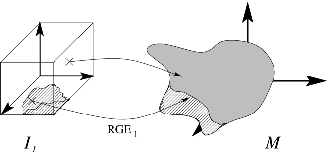
Figure 2: Back reaction of non-physicality constraints onto the input parameters. Any point in the measurement space $\mathcal{M}$ that is found to violate experimental bounds will not be part of the footprint. This in turn implies that the input point from which it was created is not physical. Any experimental boundaries in $\mathcal{M}$ will thereby lead to transformed boundary lines in $\mathcal{I}$, which delimit a region of valid input points.

Different models will have different footprints, some of which may be disjoint, while others may overlap. However, as long as the footprints’ hypersurfaces are of much lower dimensionality than $\mathcal{M}$, as is usually the case, it will be quite unlikely that there will be any overlap between the prints. As soon as it is established that the two prints are disjoint, it is possible to conclude that the two models can in principle be distinguished experimentally, as long as a certain measurement accuracy can be achieved. Fig. 1 shows that this can be established by finding that the smallest vector $\vec{v}$ still has a size greater than zero.

2.1 Distance Measure

In our previous paper [3], we looked for the closest approach of models in the space spanned by dimensionless mass ratios, where $\vec{v}$ was well defined as the smallest Euclidean distance possible. To make a more general statement possible, we now want to plot the model footprints using the masses directly. The smallest Euclidean distance is not such a suitable measure anymore, since all calculated sparticle masses are roughly proportional to the input value $m_{3/2}$, and the resulting vector $\vec{v}$ would always be the one closest to the origin.

Instead, let us look at relative distance. In the one-dimensional case we define this relative distance of two points $A$ and $B$ along one dimension to be

$$\delta=\frac{|a-b|}{a+b}\,;\qquad a,b>0\,.$$ (1)

This automatically guarantees $\delta\in[0,1)$, and the minimum value of $\delta$, if found, can be seen as the relative measurement accuracy required to definitely distinguish the points $A$ and $B$. A distance measure such as this one scales as a constant fraction if one increases both $a$ and $b$ in the same ratio. It is therefore useful because it gives a reasonable relative weight to the different variables one wishes to include in the distance measure. We imagine that $A$ and $B$ are the closest pair of points that can be predicted each by a particular different model. Supposing one measured the observable to have value $a$. If the fractional experimental uncertainty (to some chosen confidence level, for example 2$\sigma$) is smaller than $\delta$ the two points are obviously resolved by the measurement, therefore the models are discriminated. Therefore $\delta$ is a measure of the level of discrimination needed.

We now extend this interpretation to multiple dimensions. Let $A$ and $B$ be represented by $\vec{a}$ and $\vec{b}$:

$$\Delta=\frac{|\vec{a}-\vec{b}|}{|\vec{a}+\vec{b}|}=\sqrt{\frac{(a_{1}-b_{1})^{2}+\cdots+(a_{D}-b_{D})^{2}}{(a_{1}+b_{1})^{2}+\cdots+(a_{D}+b_{D})^{2}}}.$$ (2)

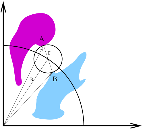
Figure 3: Geometrical measure of distance. The dark and light blobs represent the footprints of two different models to be distinguished in the measurement space $\mathcal{M}$, two dimensions of which are depicted.

$\Delta$ is the direct extension of eq. 1 to more than one dimension, with a geometric interpretation $\Delta=r/R$ (see fig. 3): Let us introduce $M$ as the midpoint of $A$ and $B$. Then $R$ is the radius of the hypersphere around the origin which passes through $M$, and $r$ is the radius of the hypersphere around $M$ with the diameter $AB$. This property makes the $\Delta$-measure invariant under rotations of the coordinate system. $\Delta$ gives us only a rough idea of the relative accuracy one needs to separate the models. The precise meaning of $\Delta$ in terms of measurements upon observables depends upon the details of the particular case under study (for example, whether the footprints are convex or not, or aligned with an axis). At point $B$, measuring the combination of observables in the direction of $\vec{v}$, where $\vec{v}=\vec{a}-\vec{b}$, to a precision better than $\Delta$ guarantees separation of the two points. Other measures sharing some of these properties could be conceived.

2.2 Function minimisation

We may view the “length” of $\vec{v}$ to be a function of two sets of input parameters. For our example case this might be

$$|\vec{v}|=f(I_{1},I_{2})\equiv f\big{(}(z_{i})_{1},(z_{i})_{2}\big{)}\,,$$ (3)

i.e. we can express our problem in terms of a scalar function of the free parameters whose function value is to be minimised. The internal workings of the function

$$f(I_{1},I_{2})=\frac{\left|\vec{A}(I_{1})-\vec{B}(I_{2})\right|}{\left|\vec{A}(I_{1})+\vec{B}(I_{2})\right|}$$ (4)

are irrelevant as far as the search algorithms are concerned.

Now that we have reduced the problem to the maximisation of a function, one might expect the application of standard techniques to provide the answer. However, these techniques had technical problems that rendered them insufficient to solve the problem. Performing a scan in every input parameter would of course work, provided a fine enough scan was done. However, there are too many input parameters for such a scan to be completed in a reasonable amount of time. Maximisers that calculate a derivative of the function such as Minuit [13] in order to implement a “hill climbing” algorithm also fail. The reason for this is the back reaction displayed in Fig. 2. There are many regions which cannot be predicted in advance, where the derivative does not exist because the region of parameter space is unphysical and no spectrum can be calculated. Efforts to get around this problem by assigning a “penalty” factor to $\Delta$ in unphysical parts of parameter space failed because the maximiser calculated a spurious derivative and either oscillated between physical and unphysical parts of parameter space, or got “stuck” in unphysical space.

3 Genetic Algorithms

One powerful set of tools does not suffer from any of the drawbacks mentioned above that made the deterministic minimisation search by Minuit so ineffective. These are genetic algorithms (GAs). In the following, at first we introduce GAs [1] using an example problem, and briefly show the mathematical background behind their success.

3.1 Overview

Genetic Algorithms differ in several points from other more deterministic methods:

• They simultaneously work on populations of solutions, rather than tracing the progress of one point through the problem space. This gives them the advantage of checking many regions of the parameter space at the same time, lowering the possibility that a global optimum might get missed in the search.

• They only use payoff information directly associated with each investigated point. No outside knowledge such as the local gradient behaviour around the point is necessary. For our problem this is one of the main advantages compared to Minuit, where the calculation of the local gradient takes a large effort in computing time. It also makes the GA robust against points that are undefined.

• They have a built-in mix of stochastic elements applied under deterministic rules, which improves their behaviour in problems with many local extrema, without the serious performance loss that a purely random search would bring.

All the power of genetic algorithms lies in the repeated application of three basic operations onto successive generations of points in the problem space. These are

1. Selection,

2. Crossover and

3. Mutation.

In the following, a simple example shall illustrate their operation.

3.2 An Example

As a simple problem, let us consider the maximisation of $f(x)=x^{2}$ on the integer interval $x\in[0,31]$ (our example follows the discussion in [1]). A simple analytic problem like the given one can of course be solved much more efficiently by straightforward hill climbing algorithms. The strength of GAs only really shows in problems that are generally hard for deterministic optimisers. For the purpose of an introduction into the mechanisms of a GA this will be sufficient, though.

3.2.1 Encoding

We need to encode our problem parameter $x$ into a string, the chromosome, on which the GA can then operate. One frequent choice is a straightforward binary encoding, where $x=1$ codes as 00001 and $x=31$ as 11111. In problems with more than one input parameter, the chromosome can simply be formed by concatenating each parameter’s string. For the example presented here, we illustrate with binary encoding, which is particularly easy to follow. Later, however, we find that a real valued encoding is more useful to solve our problem.

3.2.2 Initial Population

After this initial design decision, the first real step in the running of a GA is the creation of an initial population with a fixed number of individuals $i=1,\,\ldots,\,N$ (table 1).

$i$	Genotype	Phenotype $x_{i}$	Fitness $f_{i}=f(x_{i})$	$f_{i}/\sum{f_{i}}$
1	01101	13	169	0.14
2	11000	24	576	0.49
3	01000	8	64	0.06
4	10011	19	361	0.31

Table 1: Randomly generated starting population. $i$ labels each individual. Their genotypes (chromosomes) are assigned randomly, and are translated into the phenotype value according to the chosen encoding method. The fitness is then calculated with the function that we want to maximise: $f(x)=x^{2}$. The last column shows the fitness values normalised to 1. The colours shall make it easier to follow the propagation of these genes throughout the subsequent generations in this example.

To make this example tractable, we use a population size of only four. Real applications regularly use populations with 50–100 individuals or more. They would also usually have larger chromosome sizes.

Each individual in this first population is given a randomly generated chromosome which then represents its genotype. Note that this random assignment of genotypes only happens in the first generation, but not in the subsequent ones. According to the encoding we have chosen, each chromosome implies for its owner a phenotype $x_{i}$. The fitness of each individual is in turn a function of this phenotype. This fitness value must be positive definite, and the choice of fitness function must be such that the problem’s best solutions should be the ones with the highest fitness. Since our problem is a maximisation with positive function values only, we can take $f(x)$ directly as the fitness function. The last column in table 1 shows the normalised fitness, which will be used shortly.

To solve our optimisation problem we now need rules that tell us how to obtain the following generation from the present one. These rules of course should also guarantee some improvement in the solutions over successive generations.

3.2.3 Selection

The first operator to be applied is selection. It should ensure that individuals with higher fitness will have a larger chance of contributing offspring to the next generation. Several different selection operators can be used, here we will use one that tries to model the selection we find in natural evolution. The child population in a basic GA is fixed to have the same number of individuals as the parent population, so we need to repeat the selection of two individuals who will act as parents for two children, until we have picked $N/2$ breeding pairs. In this procedure, an individual of average fitness should be selected about once, while individuals with higher/lower fitness should be selected more/less frequently.

One selection method that achieves this is roulette wheel selection. A visual interpretation is the following: Fix a needle onto the centre of a pie chart of all individuals, where the size of each sector is proportional to that individual’s fitness (see fig. 4).

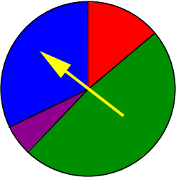
Figure 4: Roulette wheel selection.

Each individual in the parent population (table 1) is assigned a sector of the circle, with the distended angle in proportion to its fitness. Now the needle, which is assumed to end up in any position with uniform probability, is turned $N$ times. Each time, the pointed-to individual is selected into the breeding pool, where they are paired up. Obviously, individuals with larger fitness will turn up in the breeding pool more frequently. A self-pairing is possible and permitted. Since fitter individuals will distend a larger angle on the pie chart, they have a larger chance of being selected. To continue the example, let us assume that in the four spins of the wheel the following parents were chosen: 1, 2, 2 and 4. Note that individual 2 was chosen twice, while 3 does not appear at all. This corresponds nicely with the respective fitnesses.

3.2.4 Crossover

The crossover operation is necessary to obtain a child generation that is genetically different from the parents. The parents that were selected in the previous step are paired up randomly (${1}\longleftrightarrow{{2}}$ and ${{2}}\longleftrightarrow{{4}}$) and a crossover site $s$ within the chromosome is randomly chosen for each pair. Let us assume that this was $s_{1}=4$ and $s_{2}=2$ for the two breeding pairs respectively.

The chromosomes of both parents are cut after that position (see table 2), and the ends are exchanged to form the chromosomes for the two children. Table 3 shows the new generation.

Breeding pair 1			Breeding pair 2
$i$	before	after	$i$	before	after
1	0110|1	0110|0	2	11|000	11|011
2	1100|0	1100|1	4	10|011	10|000

Table 2: Crossover operation on the selected parents. The crossover site was randomly chosen to be $4$ and $2$ respectively. The parts of the chromosomes after the crossover site get swapped to create two new chromosomes which constitute the genotypes for the two children.

$i$	Genotype	Phenotype $x_{i}$	Fitness $f_{i}=f(x_{i})$	$f_{i}/\sum{f_{i}}$
5	01100	12	144	0.08
6	11001	25	625	0.36
7	11011	27	729	0.42
8	10000	16	256	0.14

Table 3: First child generation after selection and crossover. In comparison with table 1, the best solution has gone up from a fitness of $(\max f_{i})=576$ to $(\max f_{i})=729$, the average fitness has gone up from $\bar{f_{i}}=292.5$ to $\bar{f_{i}}=438.5$. This rapid increase of fitness over the very first few generations is a common feature of GAs.

In principle, one could now go back to section 3.2.3, taking the child generation as the new parents, and start selecting the next breeding pairs. This ignores one danger: if one position in the chromosomes is set to the same value in all the individuals by accident, the crossover operator will not change that fact and one whole subset of the problem space will not get visited by the GA. The final operator solves this problem.

3.2.5 Mutation

With a small probability (0.01 – 0.001) every bit in every chromosome is flipped from 1 to 0 or reverse. This operator is usually applied to all chromosomes after crossover, before the fitnesses of the new generation are evaluated. Over the span of several generations then, even a stagnated chromosome position can become reactivated by mutation.

Even after only one generation one can observe the effects that make GAs work. Crossover of individuals 2 and 4 has produced a child of new higher fitness, already quite close to the theoretical optimum. Also notable is the increase in average fitness from 292.5 to 438.5. This is a general feature in GAs, the maximum fitness already approaches the optimal value within the first few generations, the average fitness is not far behind.

3.3 Schemata make GAs work

The theoretical concept behind the success of GAs is the concept of patterns or schemata within the chromosomes [1]. Rather than operating on only $N$ individuals in each generation, a GA works with a much higher number of schemata that partly match the actual chromosomes.

A chromosome like 10110 matches $2^{5}$ schemata, such as **11*, ***10 or 1*1*0, where * stands as a wild card for either 1 or 0. Since fit chromosomes are handed down to the next generation more often than unfit ones, the number of copies $n_{S}$ of a certain schema $S$ associated with fit chromosomes will increase from one generation to the next:

$$n_{S}(t+1)=n_{S}(t)\cdot\frac{\bar{f}(S)}{\bar{f}_{\mathit{total}}},$$ (5)

where $\bar{f}(S)$ is the average fitness of all individuals whose chromosomes match schema $S$, and $\bar{f}_{\mathit{total}}$ is the average fitness of all individuals. If we assume that a certain schema approximately gives all matching chromosomes a constant fitness advantage $c$ over the average

$$\bar{f}(S)\equiv(1+c)\cdot\bar{f}_{\mathit{total}},$$ (6)

we get an exponential growth in the number of this schema from one generation to the next:

$$\quad n_{S}(t)=n_{S}(0)\cdot(1+c)^{t}.$$ (7)

Equation 5 needs to be corrected for the effects that crossover and mutation may have. To do this we need to define two measures on schemata:

• The defining length $\delta$ is the distance between the furthest two fixed positions. In the examples above, we get $\delta=1$ for **11* and ***10, and $\delta=4$ for 1*1*0.

• The order $o$ of a schema is the number of fixed positions it contains. In the above example $o$ is 2, 2 and 3 respectively.

With these measures and $L$ as the total length of a chromosome, we can now write

$$n_{S}(t+1)\geq n_{S}(t)\cdot\frac{\bar{f}(S)}{\bar{f}_{\mathit{total}}}\left[1-\frac{\delta(S)}{L-1}-o(S)\cdot p_{m}\right].$$ (8)

The first correction term in the square brackets includes the effect of crossover on the schema we are counting. With a probability of $\frac{\delta(S)}{L-1}$, the crossover site lies within the schema and the schema may get destroyed. Of course, some crossovers will preserve the schema even in that case, namely when by chance the partner in the crossover provides the right bits in the right positions. Therefore equation 8 only gives a lower bound for the number of schema $S$ in the new generation.

The final term is the effect of mutation on a schema. In a schema of order $o$, there is a probability of $(1-p_{mut})^{o}$ that the schema survives mutation. For small $p_{mut}$, as is usually the case, one can write $(1-p_{mut})^{o}\approx(1-o\cdot p_{mut})$.

A consequence of equation 8 is that short, low-order schemata of high fitness are building blocks toward a solution of the problem. During a run of the GA, the selection operator ensures that building blocks associated with fitter individuals propagate throughout the population. The crossover operator ensures that with time, several different good building blocks come together in one individual to bring it closer to the optimal solution. One can show that in a population of size $N$, approximately $\mathcal{O}(N^{3})$ schemata are processed in each generation [1].

3.4 Advanced Operators

The basic GA we have just introduced can be extended in many ways to address specific problems. Variations are possible at almost any step, but we describe here the variations that we found useful in solving our function maximisation problem. The approach that worked best was a modification of the Breeder Genetic Algorithm presented in [14]. It uses a real valued encoding of the problem parameters rather than the binary encoding presented before. This also requires an adapted set of selection, crossover and mutation operators. The following will summarise the choice of operators that worked best for our problem.

Encoding:

One chromosome consists of eight real numbers, directly representing the input parameters (these are disscussed later, see table 4 on page 4). Therefore, no decoding step is neccessary: the phenotype is directly equivalent to the chromosome.

Selection:

Instead of the stochastic roulette selection mentioned earlier, which can be seen as a model of natural selection, we use truncation selection which models the way a human breeder might select promising candidates for mating. All individuals in a generation are sorted according to their fitness and only the top third of individuals is taken to form the breeding pool. There they are paired up randomly and offspring is produced through crossover (see below) until a child population of equal size to the parent population has been created. Self-mating in the breeding pool is not permitted. To prevent a degradation in the maximal fitness already achieved, the best individual of the parent generation is copied into the child generation unchanged.

Crossover:

Crossover is implemented as intermediate recombination. Take the chromosomes of both parents to represent two points $A$ and $B$ in their eight-dimensional parameter space. Now imagine a hypercube aligned with the coordinate axes, with $A$ and $B$ at the endpoints of the longest diagonal. The child’s chromosome will then be picked at random from within this hypercube.

Mutation:

After creation of one child chromosome by crossover, the mutation operator is applied to each one of the eight parameters in the chromosome with a probability of $0.25$. If a value $x$ is to be mutated, a shift $\delta x$ is either added or subtracted from $x$ with equal probability. $\delta x$ is determined anew every time it is used through

$$\delta x=R\cdot\sum_{i=1}^{20}\left(2^{-i}\cdot P_{0.05}\right)\,;\qquad P_{0.05}=\left\{{1\mbox{ with probability }0.05}\atop{0\mbox{ with probability }0.95}\right.\,,$$ (9)

where $R$ is the range from the smallest permitted value for $x$ to the largest permitted one. It is possible for the mutated $x$ to lie outside the permitted range. If this happens, $x$ is reset to the minimum or maximum allowed value respectively. Note that the definition for $\delta x$ creates small perturbations much more often than large ones. This leads to a good search behaviour in finding an optimum locally, but also to a good coverage of the full parameter space.

We found this set of operators to give the best convergence behaviour for our problem. To completely state all GA related data here, we have run the algorithm with a population size of 300. The runs were stopped when no more improvement in maximal fitness happened for the last 20 generations.

4 Explicit Examples

We choose the models discussed in Refs. [3, 8] as candidates to discriminate. This choice is arbitrary, intended just to exemplify the technique, which should apply in principle to any models. We note in passing that using the masses is also an arbitrary choice, and in principle one could choose any observables as the dimensions of space $\mathcal{M}$. For concreteness we are using models that have been studied in type I string theory in which the source of supersymmetry breaking are either the dilaton field $S$, the overall size of the internal manifold $T$ and a blowing-up mode $B$. A combination of their $F$-terms break supersymmetry and they can be parametrised by two goldstino angles:

$$\left(\begin{array}[]{c}F^{S}\\ F^{T}\\ F^{B}\end{array}\right)=\left(\begin{array}[]{c}\sin\theta\\ \cos\theta\sin\phi\\ \cos\theta\cos\phi\end{array}\right)F_{total},$$ (10)

where $F_{total}=\sqrt{(F^{S})^{2}+(F^{T})^{2}+(F^{B})^{2}}$.

4.1 The scenarios

In this section we want to summarise the three scenarios that will be used in the remainder of the work. First, the soft breaking terms for all three are:

$$m_{0}^{2}=m_{3/2}^{2}\left(1-\cos^{2}\theta\sin^{2}\phi\right)\,,$$ (11)

$$M_{a}=\sqrt{3}m_{3/2}{\alpha_{a}\over\alpha_{\mathrm{GUT}}}\left(\sin\theta-{\beta_{a}\over 4}\alpha_{\mathrm{GUT}}\,\cos\theta\left({-10\over\sqrt{3}}\sin\phi+\cos\phi\right)\right)\,,$$ (12)

$$A_{\alpha\beta\gamma}=-\sqrt{3}m_{3/2}\sin\theta\,.$$ (13)

$m_{0}$ is a flavour-family universal scalar mass, $M_{a=1,2,3}$ the mass of the U(1), SU(2)_L and SU(3) gauginos respectively. Defining a Yukawa coupling $Y_{\alpha\beta\gamma}$, $A_{\alpha\beta\gamma}Y_{\alpha\beta\gamma}$ (no summation on repeated indices) is the trilinear interaction between scalars denoted by $\alpha\beta\gamma$. $\beta_{a}$ is the RGE $\beta$ function of gauge group $a$. As free parameters in the SUSY breaking sector, we have now $\theta$, $\phi$ and $m_{3/2}$. Additionally, $\tan\beta$ and the sign of $\mu$ are free parameters which are chosen in order to fix $m_{3}^{2}$ and $|\mu|$ (in the notation of Ref. [10]) from the minimisation of the MSSM Higgs potential and $M_{Z}$.

Note that the scalar masses and the trilinear $A$-terms are universal and quite straightforward. Their values at the high scale also do not depend on the choice of gauge unification behaviour. The gaugino masses, however, do depend on the different gauge running behaviours, as one would expect, through their dependence on $\alpha_{a}$ and $\alpha_{GUT}$. This leads us to the three model scenarios and their abbreviations which will be frequently referred to from now on:

• The GUT scenario, with the string scale at $M_{S}=2\times 10^{16}\,\mathrm{GeV}$ and the standard MSSM particle content. In this scenario we chose the usual unified gauge coupling $\alpha_{a}=\alpha_{GUT}=1/25$ as input for the soft terms. This will not make the soft gaugino masses universal, as they still contain the dependence on $\beta_{a}$.

• The early unification scenario EUF, where $M_{S}=5\times 10^{11}\,\mathrm{GeV}$. To make unification work at this scale, we have added $2\times L_{L}+3\times e_{R}$ vector-like representations to the MSSM particle spectrum. We assume that their Yukawa couplings are negligible. Their effects are set to modify the one-loop beta function coefficients $\beta_{1},\beta_{2}$ above a scale of $1\mathrm{TeV}$. This happens to be the simplest possible additional matter content that achieves the desired effect. There are models that contain possibly suitable candidates for such extra fields. Here $\alpha_{a}=\alpha_{GUT}=1/21$.

• The mirage scenario MIR [15]. The fundamental string scale is again $M_{S}=5\times 10^{11}\,\mathrm{GeV}$, but now the gauge couplings are set independently to $\alpha_{1}=1/37.6$, $\alpha_{2}=1/27$ and $\alpha_{3}=1/19.8$, while $\alpha_{GUT}=1/25$ remains at the usual GUT value.

To predict sparticle masses from these scenarios, we must solve the renormalisation group equations (RGEs) starting from a theoretical boundary condition parameterised by the string scale $M_{S}$, the goldstino angles $\theta$ and $\phi$, the ratio of Higgs VEVs $\tan\beta$, and the gravitino mass $m_{3/2}$. Constraints from experiments and cosmology (if a version of $R$-parity is conserved, as assumed here) restrict the models further.

4.2 Constraints

We use the following experimental constraints to limit the scenarios [16, 17]:

$$m_{\tilde{\chi}^{0}_{1}}>45\,\mathrm{GeV}\qquad m_{\tilde{\chi}_{1}^{\pm}}>103\,\mathrm{GeV}\qquad m_{h_{0}}>113.5\,\mathrm{GeV},$$ (14)

$$-4.2<\delta a_{\mu}\times 10^{10}<41.3\,.$$ (15)

Also, the neutralino must be the LSP. Any parameter choice violating one or more of these constraints is considered to be outside the footprint. Throughout the whole analysis $\mu>0$ and $m_{t}=175\mathrm{GeV}$ were assumed [16]. Negative $\mu$ leads to a negative $\delta a_{\mu}$ SUSY contribution, which is limited from the measurement of $(g-2)_{\mu}$ [19, 20] to be small in magnitude. This means that, for a given value of $\tan\beta$, the sparticles must be heavy in order to suppress their contribution to $\delta a_{\mu}$. In this limit, effects of the sign of $\mu$ upon the mass spectrum are suppressed. We can therefore safely ignore the $\mu<0$ case because its resulting spectra will be included in our $\mu>0$ results.

Table 4 shows the default ranges allowed for the parameters. It also summarises the other parameters that were kept constant. $m_{3/2}$ is restricted not to be too big, since then one introduces too much fine tuning in the Higgs sector of the MSSM [12], $\tan\beta$ is bounded from above by the constraint of perturbativity of Yukawa couplings up to $M_{i}$ or $M_{GUT}$, and from below by LEP2 Higgs data [17]. $\theta>30{}^{\circ}$ is chosen to avoid a situation where anomaly-mediated SUSY breaking effects are comparable to gravity mediated ones, for which the pattern of soft SUSY breaking terms is currently unknown.

$\theta$	$\phi$	$m_{3/2}$	$\tan\beta$	$\mu$	$m_{t}$	$M_{GUT}$	$M_{I}$
30–90∘	0–90∘	50–1500	2–50	$>0$	175	$2\times 10^{16}$	$5\times 10^{11}$

Table 4: Summary of parameters. The first four parameters are scanned over, and their range is given. The value of the others is kept constant except for $\mu$ which is constrained to give the correct value of $M_{Z}$. All massive parameters ($m_{3/2},m_{t},M_{I},M_{GUT}$) are given in units of GeV.

5 Results

As maximisation criterion for the genetic algorithm we use the inverse of the relative distance $\Delta$, which we defined earlier (2). In our scenarios, this quantity is built from the sparticle masses at two model points $A$ and $B$ as follows:

$$\mathit{Fitness}\equiv\frac{1}{\Delta}=\frac{|\vec{M}_{A}+\vec{M}_{B}|}{|\vec{M}_{A}-\vec{M}_{B}|}=\sqrt{\frac{\bigg{(}M_{\tilde{\chi}^{0}_{1},\,A}+M_{\tilde{\chi}^{0}_{1},\,B}\bigg{)}^{2}+\ldots+\bigg{(}M_{\tilde{\tau}_{2},\,A}+M_{\tilde{\tau}_{2},\,B}\bigg{)}^{2}}{\bigg{(}M_{\tilde{\chi}^{0}_{1},\,A}-M_{\tilde{\chi}^{0}_{1},\,B}\bigg{)}^{2}+\ldots+\bigg{(}M_{\tilde{\tau}_{2},\,A}-M_{\tilde{\tau}_{2},\,B}\bigg{)}^{2}}}\;.$$ (16)

The full list of masses we used can be found in table 6.

The GA is run until no improvement is seen for 20 generations in a row, with populations of 300 individuals. We initially found that runs using binary coding were unstable: successive runs with different random initial conditions gave significantly different fitnesses. We therefore switched to the real encoding mentioned in section 3.4, which we find to work. An important criterion is that the method can tell when two models are truly non-distinguishable, i.e. their footprints overlap: We should see large fitness values of the order of the inverse numerical precision of the calculation.

Figure 5: GA Progress in model discrimination: (a) control samples for GUT-GUT (gg), early unification - EUF (ee) and mirage-mirage (mm) “discrimination”, (b) mirage-early unification, (c) GUT-mirage, (d) GUT-early unification. The evolution of the best individual’s fitness with generation is plotted.

Fig. 5a illustrates that this is indeed is the case when we choose the two models to be identical. The numerical precision of the SOFTSUSY calculation was set to $10^{-5}$, and we obtain fitnesses of order the inverse of this number in each case. Three separate runs were tried for the GUT scenario (gg), two for the early unification (ee) and two for the mirage unification scenarios (mm). Each run was started with independent random numbers. We see that in each case a large fitness, $\mathcal{O}(10^{5})$ results. The progress of the discrimination runs show a different pattern, as shown in Figs. 5b–d for mirage-early unification, GUT-mirage and GUT-early unification discrimination respectively. In each case, six independent runs are tried and in each case we see that the fitness converges to a stable value after 100–500 generations. The rate of progress in early generations varies depending upon the random numbers used to seed the algorithm, but each separate run converges to the same value. The fitnesses in the discrimination runs are much lower than in the control run (Fig. 5a), indicating that the three footprints in $\mathcal{M}$ are disjoint. As an example, we show the input parameters for the best pairs in the 6 different runs for the GUT-EUF discrimination (Table 5).

Model	GUT						EUF
Run	1	2	3	4	5	6	1	2	3	4	5	6
$\theta$	51	49	49	50	51	49	85	77	76	81	85	85
$\phi$	35	40	40	41	39	28	51	34	31	49	58	25
$\tan\beta$	4.8	5.1	3.8	4.8	4.5	8.0	3.3	3.4	2.9	3.3	3.2	4.2
$m_{3/2}$	0.85	1.10	1.14	1.02	0.99	0.97	0.82	1.05	1.09	0.97	0.96	0.93
Max. fitness	122	119	121	120	121	109	122	119	121	120	121	109

Table 5: Input parameters of closest points (smallest $\Delta$) in 6 independent GUT-early unification discrimination runs. The angles $\phi,\theta$ are listed in degrees and $m_{3/2}$ is listed in TeV.

Although the fitnesses of the solutions are similar in independent runs (within one plot), the actual positions in the input parameters (and the observables) are different. This occurs because of approximately degenerate minima, whenever the boundaries of two footprints in $\mathcal{M}$ are roughly parallel in some region of the parameter space.

	MIR	EUF	MIR	EUF	MIR	GUT	GUT	EUF
$\theta$	42.2	77.2	45.4	87.5	51.2	66.2	51.1	85.3
$\phi$	33.2	36.3	24.4	0.2	33.2	57.9	35.4	51.1
$\tan\beta$	3.4	4.2	3.3	3.9	3.1	6.1	4.8	3.3
$m_{3/2}$	1194	991	1080	937	979	810	845	820
$\widetilde{\chi}^{0}_{1}$	673	657	603	585	613	619	551	532
$\widetilde{\chi}^{0}_{2}$	1158	1156	1099	1095	1093	1062	941	962
$\widetilde{\chi}^{0}_{3}$	1639	1652	1642	1658	1632	1685	1536	1499
$\widetilde{\chi}^{0}_{4}$	1650	1661	1652	1666	1642	1692	1543	1509
$\widetilde{\chi}^{\pm}_{1}$	1158	1156	1098	1095	1093	1062	941	962
$\widetilde{\chi}^{\pm}_{2}$	1649	1661	1651	1665	1641	1691	1542	1508
$h^{0}$	115	119	114	118	113	121	119	115
$A^{0}$	2191	2178	2158	2151	2101	2067	1932	1951
$H^{0}$	2192	2178	2159	2151	2102	2067	1933	1952
$H^{\pm}$	2193	2180	2160	2153	2103	2069	1934	1953
$\widetilde{g}$	2851	2873	2830	2847	2770	2646	2362	2477
$\widetilde{u}_{L}$	2609	2631	2564	2585	2482	2526	2287	2260
$\widetilde{d}_{L}$	2610	2632	2565	2586	2483	2528	2288	2261
$\widetilde{u}_{R}$	2524	2512	2485	2474	2401	2408	2184	2161
$\widetilde{d}_{R}$	2516	2493	2479	2459	2395	2387	2166	2147
$\widetilde{t}_{1}$	1916	1859	1898	1841	1834	1752	1571	1589
$\widetilde{t}_{2}$	2363	2369	2328	2332	2258	2261	2045	2041
$\widetilde{b}_{1}$	2505	2482	2468	2448	2385	2373	2155	2138
$\widetilde{b}_{2}$	2335	2339	2298	2302	2227	2234	2017	2008
$\widetilde{\nu_{e}}$	1302	1324	1233	1257	1139	1164	1110	1106
$\widetilde{e}_{L}$	1304	1326	1235	1259	1141	1166	1113	1109
$\widetilde{e}_{R}$	1148	1122	1082	1055	976	941	929	931
$\widetilde{\nu_{\tau}}$	1302	1323	1232	1256	1138	1161	1109	1106
$\widetilde{\tau}_{1}$	1146	1119	1081	1053	974	934	925	929
$\widetilde{\tau}_{2}$	1304	1325	1234	1258	1140	1164	1111	1108
$\Delta$	0.0054		0.0055		0.0109		0.0082
Fitness	184.6		181.0		92.1		121.7

Table 6: MSSM Spectra of closest-fit points in the various comparisons. The mirage (MIR) and early unification (EUF) scenarios are shown twice, for two different (approximately degenerate) maximal fitness. We also show the closest spectra from the GUT-mirage comparison and GUT-early unification comparison. All masses are in units of GeV. The angles $\phi,\theta$ are listed in degrees.

We give examples of the observables (in this case, masses) corresponding to the closest-fit points of each footprint in Table 6. For comparison purposes, two examples are picked from MIR-EUF discrimination runs in order to show how much the MSSM spectra differ at two different closest-fit points. The spectra are similar, as is evident by comparing the columns 2 and 4 of Table 6, or columns 3 and 5. Again, this does not have to necessarily be the case (but proved to be the case in our results). We see that our intuition that $\Delta$ roughly measures the sort of fractional precision one needs to measure the observables, in order to discriminate two models, holds by comparing the spectra between the two models that are being discriminated. We also see that accurate $\widetilde{\chi}^{0}_{1}$, $h^{0}$, $\widetilde{t}_{1}$, $\widetilde{\tau}_{1}$ mass measurements are important to help discriminate between the MIR and EUF scenarios (since these show larger mass differences).

6 Conclusions

Genetic algorithms have allowed us to answer the problem of discrimination of SUSY breaking models in the following questions: what accuracy on measurements is required to reliably tell two given different SUSY breaking scenarios apart, and which are the most important variables to measure? We have studied the discrimination of three different SUSY breaking scenarios as examples, and assumed that the relevant observables are the masses. Each of these assumptions is arbitrary, and the GAs can be applied in other situations where one wants to discriminate different models using different observables. More standard approaches such as scans or hill-climbing algorithms did not yield stable solutions.

We have constructed a measure of “relative distance” that describes the relative difference between two MSSM mass spectra. This in principle uses the entire spectrum rather than some subset [3] in order to parameterise discrimination. We found that each model can be in principle discriminated from the others, in a total of 3 comparisons. Values corresponding to $\Delta$ of 0.5$\%$, 1$\%$ and 1$\%$ were found in the three comparisons, indicating that this is the rough accuracy that will be required for sparticle mass measurements and predictions [18] in order to distinguish the models. In a control sample of a model to be discriminated against itself, a fractional accuracy of $\Delta=0.001\%$ is found, corresponding to the numerical accuracy of the calculation. This indicates that the two scenarios are indeed indistinguishable, providing confidence in the method. For more precise information regarding the simultaneous accuracies that are required for discrimination, the spectra predicted by the two points with smallest relative distance must be compared. This information is difficult to use, and would become more relevant when one knows which dimensions of $\mathcal{M}$ to use (corresponding to the minimal set of measurements that need to be made). In fact, the point pairs found to have the smallest “relative distance” vary in successive runs, indicating some approximately degenerate minima.

Now that a working setup of the GA minimisation procedure has been found, many possible applications beyond the test scenario introduced here could be taken into consideration:

• First of all, before experimental data becomes available, we can compare more model footprints in exactly the way described above, and can try to find classes of models that should easily be distinguishable from others. This is of course not restricted to models motivated by string theory, but can be applied to any kind of model that makes predictions about the low-energy sparticle mass spectrum. Possibilities include different sets of gauge mediated SUSY breaking scenarios, or a comparison with models where SUSY breaking is purely anomaly mediated.

• One could also take some typical test scenarios of different models (rather than the closest ones) and test discrimination power based on what measurements various future colliders are expected to deliver.

• As soon as real sparticle measurements are available, the GAs could take on a new role. Such an actual measurement will pick out a hyperplane, a line or even a point in the measurement space (depending on how many of the masses have been determined). The experimental uncertainty will blur out these objects somewhat, leading to something quite like the footprints in the preceding chapters. Minimising $\chi^{2}$ in the MSSM for assumed SUSY breaking models has been addressed using a combination of scan and hill-climbing algorithms [21]. However, we suspect that GAs may provide a more robust solution for finding a $\chi^{2}$ minimum.

• The GA approach also leads to an elegant way of dealing with the problem of fine-tuning in this last proposal, since one could now define the footprint to contain the experimentally acceptable solutions and minimise the fine tuning within them.

These techniques may also be useful in other areas. We can mention at least two of them. First, in cosmology, due to the level of precision that the observations are achieving, particularly for the cosmic microwave background (CMB) and due to the success of inflation to explain the current observations, we are in a situation similar to the one considered here because, as in the case of supersymmetric models, there are plenty of models of cosmological inflation. An important task for the future is to find efficient ways to discriminate among different models of inflation. More generally, the parameter set having a better fit with data needs to be investigated systematically (see [22] for an interesting discussion in this direction). Genetic algorithms may be of use in this effort.

Secondly, in string theory. There is an increasing evidence that the number of string vacua is huge. Statistical techniques are actually starting to be used in order to study classes of vacua [23] and genetic algorithms may play an important role in this effort. In particular, there is an outstanding problem of how to discriminate among different compactifications and we may find genetic algorithms useful in a similar way in which we have applied them here.

Genetic algorithms have shown their robustness and power in many other widely separate fields of engineering and research, and there is no reason why theoretical particle physics should be an exception.

References

- [1] For an introduction, see D.E. Goldberg, Genetic Algorithms in Search, Optimization and Machine Learning, Addison-Wesley, 1989.
-
[2]
A. Yamaguchi and H. Nakajima, Landau Gauge Fixing Supported by Genetic
Algorithm, Nucl. Phys. 83 (Proc. Suppl.) (2000) 840, hep-lat/9909064.
GAs have also been used to train neural networks, see e.g. J. Rojo and J. I. Latorre, J. High Energy Phys. 0401 (2004) 055, hep-ph/0401047. - [3] B.C. Allanach, D. Grellscheid and F. Quevedo, Selecting Supersymmetric String Scenarios From Sparticle Spectra, J. High Energy Phys. 0205 (2002) 048, hep-ph/0111057.
- [4] B.C. Allanach, C. Lester, M.A. Parker and B. Webber, Measuring Sparticle Masses in non-universal string inspired models at the LHC, J. High Energy Phys. 09 (2000) 04, hep-ph/0007009.
- [5] G.A. Blair, W. Porod and P.M. Zerwas, Reconstructing Supersymmetric Theories at High-Energy Scales, Phys. Rev. D 63 (2001) 017703, hep-ph/0007107; G.A. Blair, W. Porod and P.M. Zerwas, The Reconstruction of Supersymmetric Theories at High Energy Scales, Eur. Phys. J. C 27 (2003) 263, hep-ph/0210058; B.C. Allanach et al, Reconstructing Supersymmetric Theories by Coherent LHC/LC Analyses, hep-ph/0403133, LHC/LC working group document.
- [6] J.A. Aguilar-Saavendar et al, TESLA: The Superconducting Electron Positron Linear Collider With An Integrated X-ray Laser Laboratory. Technical Design Report. Part 3. Physics at an Linear Collider, hep-ph/0106315.
- [7] P. Binetruy, G.L. Kane, B.D. Nelson, L.T. Wang and T.T. Wang, Relating incomplete data and incomplete theory, hep-ph/0312248.
- [8] S.A. Abel, B.C. Allanach, F. Quevedo , L. Ibáñez and M. Klein, Soft SUSY Breaking, Dilaton Domination and Intermediate Scale String Models, J. High Energy Phys. 0012 (2000) 026, hep-ph/0005260.
- [9] K. Benakli, Phenomenology of Low Quantum Gravity Scale Models, Phys. Rev. D 60 (1999) 60, hep-ph/9809582; C.P. Burgess, L.E. Ibáñez and F. Quevedo, Strings at the Intermediate Scale, or is the Fermi Scale Dual to the Planck Scale?, Phys. Lett. B 447 (1999) 257, hep-ph/9810535.
- [10] B.C. Allanach, SOFTSUSY: a Program For Calculating Supersymmetric Spectra, Comput. Phys. Commun. 143 (2002) 305, hep-ph/0106304.
- [11] H. Baer, F.E. Paige, S. Protopopescu and X. Tata, ISAJET: A Monte-Carlo Event Generator for , and Reactions, hep-ph/0001086; A. Djouadi, J.-L. Kneur and G. Moultaka, SUSPECT: A Fortran Code for the Supersymmetric and Higgs Particle Spectrum in the MSSM, hep-ph/0211331; W. Porod, SPHENO: a Program For Calculating Supersymmetric Spectra, SUSY Particle Decays and SUSY Particle Production at Colliders, Comput. Phys. Commun. 153 (2003) 275, hep-ph/0301101.
- [12] B. de Carlos and J.A. Casas, One Loop Analysis Of The Electroweak Breaking In Supersymmetric Models And The Fine Tuning Problem, Phys. Lett. B 309 (1993) 320, hep-ph/9303291; R. Barbieri and A. Strumia, About the fine-tuning price of LEP, Phys. Lett. B 433 (1998) 63, hep-ph/9801353.
- [13] F. James, MINUIT, function minimisation and error analysis, http://wwwasdoc.web.cern.ch/wwwasdoc/minuit/minmain.html
- [14] H. Mühlenbein and D. Schlierkamp-Voosen, Predictive Models for the Breeder Genetic Algorithm: I. Continuous Parameter Optimization, Evolutionary Computation 1 (1993) 25.
- [15] L.E. Ibáñez, Mirage gauge coupling unification, hep-ph/9905349.
- [16] K. Hagiwara et al. [Particle Data Group Collaboration], Phys. Rev. D 66 (2002) 010001.
- [17] R. Barate et al. [LEP collaborations], Phys. Lett. B 565 (2003) 61, hep-ex/0306033.
- [18] B.C. Allanach, S. Kraml and W. Porod, Theoretical uncertainties in sparticle mass predictions from computational tools, J. High Energy Phys. 0303 (2003) 016, [hep-ph/0302102]; B.C. Allanach, G. Belanger, F. Boudjema, A. Pukhov and W. Porod, Uncertainties in relic density calculations in mSUGRA, hep-ph/0402161; ibid in B.C. Allanach et al. [Beyond the Standard Model Working Group Collaboration], Les Houches ’Physics at TeV Colliders 2003’ Beyond the Standard Model Working Group: Summary report, hep-ph/0402295; B.C. Allanach, A. Djouadi, J.L. Kneur, W. Porod and P. Slavich, Precise determination of the neutral Higgs boson masses in the MSSM, hep-ph/0406166.
- [19] H.N. Brown et al., Muon Collaboration, Precise measurement of the positive muon anomalous magnetic moment, Phys. Rev. Lett. 86 (2001) 2227, hep-ex/0102017.
- [20] S. Narison, Muon and tau anomalies updated, Phys. Lett. B 513 (2001) 53, [Erratum—ibid. B 526 (2002) 414], hep-ph/0103199v5.
- [21] R. Lafaye, T. Plehn and D. Zerwas, SFITTER: SUSY parameter analysis at LHC and LC, hep-ph/0404282.
- [22] A.R. Liddle, How many cosmological parameters?, astro-ph/0401198.
- [23] M.R. Douglas, The statistics of string / M theory vacua, J. High Energy Phys. 0305 (2003) 046, hep-th/0303194.