Spectral density in resonance region and analytic confinement

Abstract

We study the role of finite widths of resonances in a nonlocal version of the Wick-Cutkosky model. The spectrum of bound states is known analytically in this model and forms linear Regge tragectories. We compute the widths of resonances, calculate the spectral density in an extension of the Breit-Wigner ansatz and discuss a mechanism for the damping of unphysical exponential growth of observables at high energy due to finite widths of resonances.

I Introduction

Behaviour in field theories with nonlocal interactions in the time-like momentum region is the central concern of this paper. Nonlocal quantum field theory has a long history. Initially it was invented as an attempt at solving the problem of UV divergences. However after the development of renormalisation techniques for local QFT the study of nonlocal interactions became a field of academic interest. Nevertheless the challenge of constructing self-consistent and mathematically rigorous quantum field theories with nonlocal interactions and their phenomenological application have been attracting permanent attention. As a result of this long activity of several decades the general principles of quantisation of nonlocal field theories have been formulated. Various issues related to quantisation, unitarity of the $S$-matrix, realisation of causality, the validity of Froissart-type bounds at high energy and the physical interpretation of nonlocal fields can be found for instance in  Meiman ; Fainberg ; Efimov ; Efi01 ; Moffat ; Woodard ; Leutw80 ; Efiv ; Feyn ; Blokh ; Smekal . For the present paper the essential result is that for a theory with typical growth of amplitudes in the complex momentum plane and $\Lambda$ the scale of nonlocality the Froissart type bound on the total cross-section Efi01 ,

$$\sigma_{\rm tot}(s)\leq Cs^{\kappa-1}\log^{2}s,$$ (1)

$${\cal A}\sim e^{(p^{2}/\Lambda^{2})^{\kappa}},\ \ \kappa\geq 1/2$$

can be derived assuming

• unitarity of the $S$-matrix,

• analyticity of amplitudes on the Martin-Lehmann ellipse.

These two requirements are fulfilled in local as well as in nonlocal QFT with the form factors being entire analytical functions of momenta. Despite this upper bound on the total-cross section, practically useful procedures for calculating observables at high energy in nonlocal QFT have been not formulated. Thus, since amplitudes are exponentially growing within perturbation theory, the common wisdom is that nonlocal theories necessarily display pathological behaviour at high energy, which is usually considered as a fundamental drawback of nonlocal QFT models Smekal ; Joglekar . The aim of the present paper is to give an example of such a practical calculation for the total annihilation cross section in a confining nonlocal model exhibiting a Regge spectrum of bound states. In order to decode this statement of the problem we first have to explain its context.

An essential disadvantage of nonlocal theories has always been seen in the functional ambiguity in the choice of form factors related to the nonlocal character of interactions. Though requirement of unitarity restricts the form factors to be entire analytical functions of momenta, an ambiguity within this class of form factors is unavoidable as far as nonlocality is introduced as a fundamental property of the theory. An unexpected source for a nonlocal character of quantum fields has been pointed out by Leutwyler Leutw80 who has noticed that the propagator of the massless charged scalar field in the presence of background (anti-)self-dual homogeneous gauge field takes the form

$$D(p^{2})=\frac{1-e^{-p^{2}/\Lambda^{2}}}{p^{2}},$$ (2)

here $p$ is Euclidean momentum, and scale $\Lambda$ is related to the strength of the background gauge field. The nonlocal form factor $(1-\exp(-p^{2}/\Lambda^{2}))$ appears here due to the presence of strong nonperturbative gauge fields, and thus its appearance itself and particular form can be related to the properties of the physical vacuum of the system. For vanishing field strength $\Lambda\to 0$, and the usual scalar propagator is recovered. Such an observation was immediately recognised as potentially interesting in application to the confinement problem in QCD Leutw80 . For physical interpretation it is important that the nonperturbative background gauge field eliminates the pole in the momentum space propagator of a charged field rendering it an entire analytical function. Such an analytical property of the propagator can be regarded as dynamical confinement of the charged field since it has no particle interpretation Leutw80 ; Finjord ; Efiv . It is also important that such well established perturbative properties of QCD as asymptotic freedom at short distances are unaffected by the nonlocality generated by such background gluon fields. We have here an example of a theory defined by a local classical Lagrangian but with nonlocal behaviour of the quantised fields appearing as a consequence of a nonperturbative gauge field configuration. The (anti-)self-dual homogeneous gluon field itself can be seen as a highly idealised analytically tractable realisation of more complicated and realistic nonperturbative gauge configurations responsible for confinement (for instance, the domain model NK2001 ; NK2004 is a specific attempt at realising a more detailed picture of the QCD vacuum in this spirit).

Turning to confinement specifically now, this phenomenon is more than just the absence of the coloured quark-gluon states in the physical spectrum of QCD, but the mechanism by which colourless bound states are present in the spectrum of QCD. One of the first connections between confinement and the hadron spectrum was achieved by the string picture, which provided a simple explanation for the pattern of Regge trajectories from a mechanism of confinement. However, the string explanation for Regge trajectories is not unique. Another, purely field theoretical approach to bound state formation is provided by the hadronisation procedure in the QCD functional integral which is closely connected with Bethe-Salpeter approach to the description of relativistic bound states PRC87 ; PRD95 . It has been shown within the bosonisation procedure that nonlocality in quark propagators similar to Eq. (2) generated by the homogeneous (anti-)self-dual field in QCD leads to asymptotically linear Regge trajectories  PRD95 . In fact this approach turned out to be successful in application to wide variety of meson spectra – light, heavy-light mesons and heavy quarkonia PRD96 . The specific chiral properties of quark eigenmodes are similar to those in an instanton background and are of crucial importance in the description of light mesons in this context.

In its most clean and refined form the role of nonlocality of the type Eq. (2) in generating a linear Regge spectrum of bound states has been exposed in EfGan where the method of PRD95 has been improved and applied to a scalar field model. Unlike genuine QCD with all its complications, this model allows for analytical solution of the Bethe-Salpeter equation in the one-boson exchange approximation. The Lagrangian of the model has the same structure as that of the well-known Wick-Cutkosky model WickCutkosky

$${\cal L}=-\Phi^{\dagger}S^{-1}(-\partial^{2})\Phi-\frac{1}{2}\phi D^{-1}(-\partial^{2})\phi-g\Phi^{\dagger}\Phi\phi.$$ (3)

The Wick-Cutkosky model corresponds to a standard real massless scalar field $\phi$ and massive charged scalar field $\Phi$. It was invented as a prototype theory for studying the relativistic bound state problem in quantum electrodynamics. It turned out that the choice of Euclidean momentum space propagators of the form

$$S(p^{2})=D(p^{2})={1\over{\Lambda^{2}}}e^{-p^{2}/\Lambda^{2}}$$ (4)

leads to a Bethe-Salpeter equation which is analytically soluble in the one-boson exchange approximation generating a Regge spectrum of relativistic bound states EfGan with mass-squared

$$M_{nl}^{2}=M_{0}^{2}+(2n+l)\ln(2+\sqrt{3})^{2}\Lambda^{2},$$ (5)

which is linear both in radial number $n$ and angular momentum $l$. Thus the model given by Eqs.(3) and (4) can be seen as a soluble prototype of a confining theory, here with confined fundamental fields $\phi$ and $\Phi$ and a Regge spectrum of relativistic bound states representing the physical particle spectrum. It is remarkable that the effective action for the composite fields describing the bound states can also be derived analytically within the bosonisation approach, thus enabling further calculations of physical quantities such as form-factors, decay widths, and scattering cross-sections. The more realistic choice

$$S(p^{2})\sim D(p^{2})\sim\frac{1-e^{-p^{2}/\Lambda^{2}}}{p^{2}},$$ (6)

where nonlocality appears as an (exponentially small at short distances) correction to the local massless propagators, allows a variational approximate solution of the corresponding Bethe-Salpeter equation and displays an asymptotically linear Regge spectrum EfGan .

In this paper we consider the total annihilation cross section in the model of Eqs.(3) and (4) using the method suggested in Shif , where a similar problem has been studied in application to the ’t Hooft model. The total cross section for annihilation of a lepton-anti-lepton pair into hadrons via a scalar “photon” was evaluated in Shif by means of continuation of Breit-Wigner formulae in the complex plane using the fact that the physical spectrum of the ’t Hooft model consists of a Regge spectrum of hadronic resonances with the finite widths. In our case the bound states form a physical Regge spectrum of resonances and the effective “hadron” action is known explicitly. The scattering problem can be formulated in a standard way for these hadrons and a unitary $S$-matrix can be defined. The total cross section is calculated by means of the optical theorem, namely via the imaginary part of the correlator of two scalar currents

$$\Pi(q)=\int d^{4}xe^{iqx}\langle 0|j(x)j(0)|0\rangle,\ \ j(x)=\Phi^{\dagger}(x)\Phi(x).$$ (7)

As in the t’Hooft model the crucial point is to incorporate into the calculation of the RHS of Eq.(7) the finite widths of the resonances of the physical spectrum. As explained below, the imaginary part of the correlator is calculated in the approximation based on an extended Breit-Wigner formula. This approximation is valid if resonances are narrow enough, which is satisfied in the model under consideration for the seven lowest resonances corresponding to the energy interval $s\lesssim 30\div 40\Lambda^{2}$.

It should be stressed that our task is not verification of the asymptotic inequality Eq.(1). At asymptotically high energy the number of resonances involved in the calculation of the total cross-section grows rapidly, their width becoming so large that they strongly overlap. In this regime an approximation based on the Breit-Wigner formula is not valid and methods in the spirit of the statistical bootstrap Hag should be more appropriate. As already stated, we intend rather to give a particular example demonstrating a computation of physical quantities at relatively high energies within a nonlocal model with confinement of fundamental fields and a Regge spectrum of bound states.

The final result for our estimate of the spectral density is given in the upper plot of Fig.5. We conclude that in a nonlocal theory with confined fundamental fields and exponentially growing amplitudes, taking into account the physical bound states can suppress unphysical growth of observable quantities at higher energies. The finite width of these resonances is of particular importance. Exponential growth of the widths is a particularly distinctive feature of the analytic confinement scenario. It leads to the convergence of the Breit-Wigner type series for the spectral function. In a broader context, as indicated in a recent paper BlB03 , exponentially growing widths of hadronic resonances can be important for understanding the phenomenology related to the quark-gluon plasma: it eliminates the divergence of the thermodynamic functions above the Hagedorn temperature and is able to successfully describe lattice QCD data for the energy density. We discuss this issue briefly in the last section.

Figure 1: Graphical representation of various terms in the effective action.

II The Effective Action for Composite Fields.

Our starting point is the Euclidean functional integral

$${\cal Z}[I]={\cal N}\int{\cal D}\phi{\cal D}\Phi{\cal D}\Phi^{\dagger}\exp\left\{\int d^{4}x\left[{\cal L}(x)-\Phi^{\dagger}(x)\Phi(x)I(x)\right]\right\},$$ (8)

where the Lagrangian ${\cal L}(x)$ is defined by Eqs.(3) and (4), and the external current $I(x)$

$$I(x)=e^{2}\int d^{4}yG(x-y)\bar{l}(y)l(y)$$

represents interaction with the scalar lepton current $\bar{l}(y)l(y)$ by virtue of scalar particle (analogous to photon) exchange reflected in the propagator $G(z)$.

The propagators $S(p^{2})$ and $D(p^{2})$ given in Eq.(4) are entire functions such that no particles can be associated with the fields $\Phi$ and $\phi$. These fields represent fluctuations localised in space and time. A typical space-time size of fluctuations is set by a confinement scale $\Lambda$. The physical particle spectrum of the system can be recovered by means of the “bosonisation” procedure applied to the functional integral Eq.(8). For a detailed description of this procedure for this case we refer the reader to EfGan . Essentially, bosonisation requires solving the Bethe-Salpeter equation in the one-boson exchange approximation, which can be done analytically due to the simple Gaussian form of propagators. The main steps are as follows. Integrating out the field $\phi$ one arrives at a quartic interaction of the scalar fields $\Phi$:

$$L_{2}[\Phi]=\frac{g^{2}}{2}\int d^{4}x_{1}d^{4}x_{2}\Phi^{\dagger}(x_{1})\Phi(x_{1})D(x_{1}-x_{2})\Phi^{\dagger}(x_{2})\Phi(x_{2}).$$ (9)

Introducing a complete orthonormal set of functions $U_{\cal Q}$, corresponding to the radial quantum number, total momentum and magnetic numbers ${\cal Q}=\{n,l,\mu\}$, the four point interaction can be rewritten as an infinite sum of products of a non-local currents

$$L_{2}=\frac{g^{2}}{2}\sum_{\cal Q}\int d^{4}xJ_{\cal Q}(x)J_{\cal Q}(x)$$ (10)

with

$$J_{\cal Q}(x) = \Phi^{\dagger}(x)V_{\cal Q}(\stackrel{{\scriptstyle\leftrightarrow}}{{\partial}})\Phi(x)$$

$$V_{\cal Q}(\stackrel{{\scriptstyle\leftrightarrow}}{{\partial}}) = \int d^{4}y\sqrt{D(y)}U_{\cal Q}(y)e^{\frac{y}{2}\stackrel{{\scriptstyle\leftrightarrow}}{{\partial}}}$$ (11)

One introduces auxiliary fields $\Psi_{\cal Q}$ with a subsequent Gaussian integration over the field $\Phi$. As a result the original functional integral (8) turns out to be identically rewritten in terms of composite fields $\Psi_{\cal Q}$ representing collective excitations in the system

$$Z = \prod_{\cal Q}\int{\cal D}\Psi_{\cal Q}\exp\left\{-\frac{\Lambda^{2}}{2}\int d^{4}p\Psi_{\cal Q}(-p)(\delta_{\cal QQ^{\prime}}-\alpha\Sigma_{\cal QQ^{\prime}}(p))\Psi_{\cal Q^{\prime}}(p)+W_{I}[g\Psi]\right\}$$ (12)

where the dimensionless coupling constant $\alpha=g^{2}/(4\pi\Lambda)^{2}$, and

$$W_{I}[g\Psi]=-{\rm{Tr}}[\ln(1-g\Psi_{\cal Q}V_{\cal Q}S-IS)+\frac{g^{2}}{2}\Psi_{\cal Q}V_{\cal Q}S\Psi_{\cal Q^{\prime}}V_{\cal Q^{\prime}}S]$$ (13)

describes interactions between composite fields from which the quadratic term in the expansion of the logarithm is subtracted and added to the original quadratic part,

$$\alpha\tilde{\Sigma}_{\cal QQ^{\prime}}(x-y)=\frac{g^{2}}{2\Lambda^{2}}V_{\cal Q}(\stackrel{{\scriptstyle\leftrightarrow}}{{\partial}}_{x})S(x-y)V_{\cal Q^{\prime}}(\stackrel{{\scriptstyle\leftrightarrow}}{{\partial}}_{y})S(y-x)$$

The nontrivial requirement is that the basis $U_{\cal Q}$ be chosen such that the self-energy $\Sigma_{\cal QQ^{\prime}}(p)$ and hence the quadratic part of the effective action is diagonal in the quantum numbers $Q$,

$$\Sigma_{\cal QQ^{\prime}}(p)=E_{\cal Q}(-p^{2})\delta_{\cal QQ^{\prime}}$$ (14)

Bound state masses are then real solutions to

$$1=\alpha E_{\cal Q}(M_{\cal Q}^{2}).$$ (15)

Diagonalisation of the self-energy is equivalent to the solution of the Bethe-Salpeter equation in the one-boson exchange approximation. In the momentum representation propagators and vertices involved in the effective action have the form EfGan

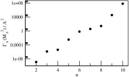
Figure 2: The two-particle decay width $\Gamma_{n}(M_{n}^{2})$ as a function of radial quantum number. Deviation from strictly exponential behaviour is due to the polynomial $P_{n}(s)$ in $\Gamma_{n}(s)\propto P_{n}(s)\exp({\rm const}\ s)$.

$$S(p) = \Lambda^{-2}e^{-p^{2}/\Lambda^{2}},$$

$$V^{nl}_{\mu_{1}\dots\mu_{l}}(K) = e^{i(q-p)x}\left[e^{ipx}V^{nl}_{\mu_{1}\dots\mu_{l}}\left(\stackrel{{\scriptstyle\leftrightarrow}}{{\partial}}_{x}\right)e^{-iqx}\right],$$ (16)

$$= (-1)^{n+l}\Lambda C_{nl}T^{l}_{\mu_{1},\dots,\mu_{l}}(K)L^{l+1}_{n}(aK^{2})e^{-bK^{2}}$$

with $K=(p+q)/2\Lambda$, $a=2\sqrt{3}$, $b=2/(1+\sqrt{3})=4/(2+a)$ and

$$C_{nl}={{2^{n+2+2l}\sqrt{3}^{l/2+1}}\over{(1+\sqrt{3})^{2n+l+2}}}\sqrt{{{n!(l+1)}\over{(n+l+1)!}}}.$$

Here the angular part of the vertex is given by $T^{l}_{\mu_{1}\dots\mu_{l}}$, the irreducible tensors of the Euclidean rotation group $O(4)$,

$$\int_{\Omega}\frac{d\omega}{2\pi^{2}}T^{l}_{\mu_{1}\dots\mu_{l}}(n_{y})T^{k}_{\nu_{1}\dots\nu_{k}}(n_{y})=\frac{1}{2^{l}(l+1)}\delta^{lk}\delta_{\mu_{1}\nu_{1}}\dots\delta_{\mu_{l}\nu_{l}}$$

$$T^{l}_{\mu_{1}\dots\mu\dots\nu\dots\mu_{l}}(n_{y})=T^{l}_{\mu_{1}\dots\nu\dots\mu\dots\mu_{l}}(n_{y}),\ T^{l}_{\mu\mu\dots\mu_{l}}(n_{y})=0,$$

$$T^{l}_{\mu_{1}\dots\mu_{l}}(n_{y})T^{l}_{\mu_{1}\dots\mu_{l}}(n_{x})=\frac{1}{2^{l}}C_{l}^{(1)}(n_{y}n_{x}),\ \ n_{x}^{2}=n_{y}^{2}=1$$ (17)

with $C_{l}^{(1)}$ being Gegenbauer polynomials. The radial part corresponds to the Laguerre polynomials $L^{l+1}_{n}$, with

$$\int_{0}^{\infty}duu^{l+1}e^{-u}L^{l+1}_{n}(u)L^{l+1}_{n^{\prime}}(u)=\delta_{nn^{\prime}}$$

Calculation of the self-energy gives

$$E_{nl}(-p^{2}) = {e^{-{{p^{2}}\over{2\Lambda^{2}}}}\over{(2+\sqrt{3})^{2n+l+2}}},$$

and the square of the bound state masses read

$$M_{nl}^{2}=2\Lambda^{2}\left[\ln\frac{(2+\sqrt{3})^{2}}{\alpha}+(2n+l)\ln(2+\sqrt{3})\right]$$ (18)

which manifests a linear Regge spectrum. Finally the fields should be rescaled

$$\Psi_{\cal Q}=\Psi_{\cal Q}g^{-1}\Lambda h_{\cal Q},$$

$$h^{-2}_{\cal Q}=\frac{\Lambda^{2}}{(4\pi)^{2}}\frac{dE_{\cal Q}(-p^{2})}{dp^{2}}\Big{|}_{p^{2}=-M^{2}_{\cal Q}}$$ (19)

in order to ensure the correct residue of the propagator at the mass pole. The coupling constant $h_{\cal Q}$ is defined as a dimensionless quantity. Thus the final form of the functional integral for composite fields is

$$Z = \prod_{\cal Q}\int{\cal D}\Psi_{\cal Q}\exp\left\{-\frac{\Lambda^{4}h^{2}_{\cal Q}}{2g^{2}}\int d^{4}p\Psi_{\cal Q}(-p)(1-\alpha E_{\cal Q}(-p^{2}))\Psi_{\cal Q}(p)+W_{I}[h_{\cal Q}\Psi]\right\}.$$ (20)

The original coupling constant $g$ enters only the quadratic part of the effective action, while the remaining terms contain the effective coupling constant $h_{\cal Q}$.

The formal functional integral (20) can be used to define a unitary nonlocal theory for the interacting fields $\Psi_{\cal Q}$ by defining the appropriate Gaussian measure for its computation. Namely, one rewrites $E_{\cal Q}(-p^{2})$ as

$$1-\alpha E_{\cal Q}(-p^{2})=(M^{2}_{\cal Q}+p^{2})\alpha E^{\prime}_{\cal Q}(M^{2}_{\cal Q})-\left[\alpha E_{\cal Q}(-p^{2})-1+(M^{2}_{\cal Q}+p^{2})\alpha E^{\prime}_{\cal Q}(M^{2}_{\cal Q})\right],$$ (21)

$$1-\alpha E_{\cal Q}(M^{2}_{\cal Q})=0.$$

This decomposition exists since $E_{\cal Q}(-p^{2})$ is an entire analytical function. If one uses now the first term of the RHS of Eq.(21) to define the standard free field Gaussian measure for computation of the functional integral then the theory of interacting composite fields $\Psi_{\cal Q}$ so defined is unitary since all nonlocal form factors in the action are entire analytical functions, and the only singularities which appear in the $S$-matrix are related to the physical particles associated with fields $\Psi_{\cal Q}$. In particular, this theory satisfies the conditions required for the derivation of the high energy bound Eq.(1) with $\kappa=1$. Such a “free field” Gaussian measure is appropriate for computing the processes in which all composite particles are almost on-shell. In this case $\left[\alpha E_{\cal Q}(-p^{2})-1+(M^{2}_{\cal Q}+p^{2})\alpha E^{\prime}_{\cal Q}(M^{2}_{\cal Q})\right]=O((M^{2}_{\cal Q}+p^{2})^{2})$ is small and can be considered as a perturbation.

Figure 3: Graphical representation of the polarisation function.

III Total cross section of $\bar{l}l$ annihilation to “hadrons”.

According to the optical theorem the total cross section for the inclusive process $\bar{l}l\to{\rm``hadrons^{\prime\prime}}$

$$\sigma_{\rm tot}(s)=\frac{1}{2s}\sum_{\cal Q}(2\pi)^{4}\delta^{(4)}(p_{\cal Q}-q)|\langle{\cal Q}|T|\bar{l}l\rangle|^{2}$$

can be expressed through the imaginary part of the amplitude for elastic forward scattering, which is proportional to the spectral density $\rho(s)$, namely the imaginary part of the correlator of two scalar currents

$$\rho(s)=\Im\int d^{4}xe^{iqx}\langle 0|j(x)j(0)|0\rangle|_{q^{2}=s},\ \ j(x)=\Phi^{\dagger}(x)\Phi(x).$$

In terms of the effective action in Eq.(12) the spectral density is given by the imaginary part of diagrams with one, two and generally $n$ intermediate “hadrons” as shown in Fig.3a-c. Since the propagator of the constituent field $\Phi$ (thin solid line) and the vertices $V_{\cal Q}$ (see Eq.(II)) are entire analytical functions no contribution to the imaginary part of diagrams in Fig.3 can come from the constituent field loops. In particular, the diagram in Fig.3d has no imaginary part and does not contribute to the spectral density.

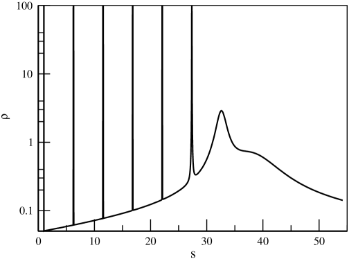
Figure 4: Spectral density in the Breit-Wigner approximation as defined by Eq.(22)

In the Breit-Wigner approximation of the resonance propagator, the contribution of diagram in Fig.3a to the spectral density takes the form

$$\rho_{BW}(s)=\sum_{n=0}^{\infty}\lim_{\varepsilon\to 0}\frac{h^{2}_{n0}g^{2}_{n0}(M^{2}_{n0})[\varepsilon+\Gamma_{n}(M^{2}_{n0})]}{[(M^{2}_{n0}-s)]^{2}+[\varepsilon+\Gamma_{n}(M^{2}_{n0})]^{2}},$$ (22)

where $\Gamma_{n}(M^{2}_{n0})$ is the width of the resonance, which is equal to zero for the lowest state. It should be noted that the expansion analogous to that in $1/N_{\rm c}$ in the ’t Hooft model or $QCD$ is represented in the model under consideration via an expansion in the number of loops which include internal resonance propagators. Further calculations will be based on this decomposition over “hadronic” loops. At this point we take this expansion as a way of classifying the various contributions, and will discuss its validity in more detail shortly. As for the leading order contributions in $1/N_{\rm c}$ in the ’t Hooft model, the bound states in the nonlocal model are stable in the zeroeth order of this expansion over “hadronic” loops. In this approximation, namely with decay widths neglected in Eq.(22), the spectral density is simply an infinite equidistant sequence of delta functions. The lowest order contribution to the widths of resonances in this loop expansion are the two-particle decays. Numerically the widths for few lowest resonances are shown in Fig.2. One can see that the width is exponentially growing with $n$, which ensures convergence of the series for the spectral density in Eq.(22) for any $s$ since

$$h^{2}_{n0}g^{2}_{n0}\propto n$$

for $n\gg 1$. The exponential growth of the decay width is precisely due to nonlocality. This should be compared with the behaviour $\Gamma_{n}\propto\sqrt{n}$ and $g_{n}\to{\rm const}$ in the ’t Hooft model or string based picture of confinement. We comment in the discussion section on whether available experimental data can distinguish between these two qualitatively different dependencies.

Summing the convergent series in Eq.(22) gives the spectral density shown in Fig.4. Qualitatively it has a reasonable form and decreases at large $s$. The advantage of the Breit-Wigner approximation for the resonance propagator is that it explicitly ensures the correct analytical properties: only physical singularities in the complex $s$-plane are present in the Breit-Wigner propagator.

However, there are three important factors at large $s$ which are missed in the spectral density calculated through the Breit-Wigner propagator with inclusion of two-particle decay widths. First of all decays to three and more particles become important at large $s$. Accounting for them would broaden the resonances and lower the spectral density. The second contribution comes from the diagrams with two or more intermediate bound states (see Fig.3b,c) which would increase the spectral density at large $s$. These two factors indicate that Eq.(22) cannot give a truly reliable result for asymptotically large $s$. At most it provides a hint at the tendency of $\rho(s)$ to decrease at larger $s$. The third factor is that the Breit-Wigner approximation is valid, strictly speaking, only in the vicinity of a resonance pole and if the resonance is narrow enough. This means for $s$ located away from the resonance position the contribution of the $n$-th resonance to the series Eq.(22) might not be reflected correctly. In terms of the effective action discussed in the previous section the Breit-Wigner approximation for the propagator corresponds to the “free field” Gaussian measure in the functional integral with the addition of the on-shell widths of resonances. It is clear that corrections coming from the second term in the RHS of Eq.(21) are not small for $p^{2}$ being off-shell. Certain resummations are necessary.

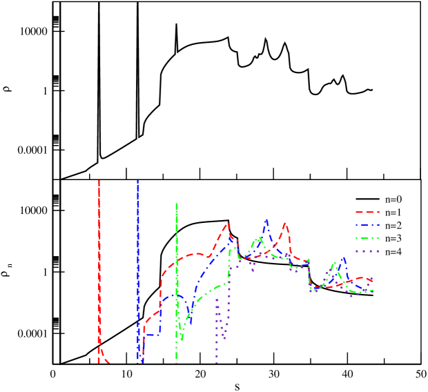
Figure 5: Spectral density $\rho(s)$ as a function of the energy variable $s$ (upper plot) and the contributions $\rho_{n}(s)$ of few lowest radial numbers to the total spectral density (lower plot)

The effective action at our disposal offers an extension of the Breit-Wigner representation, which can account for such resummations just mentioned via inclusion of the energy dependence of the self-energy $E_{n0}(s)$, the transition amplitude $g_{n0}(s)$ and the imaginary part – decay width $\Gamma_{n0}(s)$. This extension of the spectral density takes the form

$$\rho(s)=\sum_{n=0}^{\infty}\rho_{n}(s),\$$

$$\rho_{n}(s)=\lim_{\varepsilon\to 0}\frac{|g_{n0}(s)|^{2}[\varepsilon+\tilde{\Gamma}_{n0}(s)]}{[1-\alpha E_{n0}(s)]^{2}+[\varepsilon+\tilde{\Gamma}_{n0}(s)]^{2}},$$

$$\tilde{\Gamma}_{n0}=\frac{16\pi^{2}\alpha}{h_{n0}\Lambda^{2}}\Gamma_{n0}$$ (23)

where the summation spans only radial excitations with $l=0$ because of conservation of orbital momentum which is a good quantum number in this problem. The transition amplitude $g_{n0}(s)$ is given by the diagram in Fig.1b. Simple calculation gives

$$g_{n0}(s)=(-1)^{n}\sqrt{n+1}E_{n0}(s),\ E_{n0}(s)=\frac{e^{s/2\Lambda^{2}}}{(2+\sqrt{3})^{2n+2}}.$$ (24)

The quantity $\Gamma_{n0}(s)$ is the total width of two-particle decays of a resonance with orbital momentum $l=0$, radial number $n$ and squared-energy $s$. Details of the calculation of $\Gamma_{n0}(s)$ are given in the appendix.

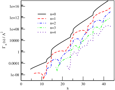
Figure 6: Two-particle decay widths $\Gamma_{n}(s)$ as a function of energy variable $s$ for the few lowest resonances.

Numerical results for $\Gamma_{n0}(s)$ are given in Fig.6, which shows its exponential growth with $s$, and

$$\Gamma_{n0}(s)\gg g_{n0}(s)\propto E_{n0}(s)$$

for large $s$. This inequality results in the behaviour of the separate terms $\rho_{n}(s)$ shown in the lower plot in Fig.5. Summing up these terms gives the spectral density shown in the upper plot in Fig.5. Qualitatively this spectral density reproduces the character of the simple Breit-Wigner approximation, Fig.4. The oscillations seen in $\rho_{n}(s)$ in Fig.5 additional to the resonance peaks are reflections of two features. The first is the corresponding oscillations in $\Gamma_{n}(s)$ in Fig.6 which are due to the opening of new decay channels at certain values of $s$. The second, and more important, cause is the functional structure of the amplitude ${\cal A}_{n}(s)$ (see appendix): essentially it is a product of a polynomial and exponent in $s$. Again the spectral density shows several sharp peaks corresponding to the lowest narrow resonances, then it has a maximum and a tendency to decrease at higher energy. It should be stressed that $\rho(s)$ is limited by the region of not very large values of $s$ because of the same as for $\rho_{\rm BW}(s)$ two reasons (decays into more than two final states and diagrams with two or more intermediate resonances). However unlike the plain Breit-Wigner approximation the extended formulae for the propagator should be more appropriate for the values of $s$ away from resonance position although only in the vicinity of the real axis in the complex $s$-plane. The reason preventing it from being a good approximation in the whole complex plane is hidden in the property of entire functions which have infinitely many zeroes in the complex plane. In addition to the desirable physical pole corresponding to the resonance, the extended propagator has artificial unphysical poles for complex values of $s$. As soon as these poles are sufficiently far from the real axis and do not noticeably affect the form of $\rho(s)$ the approximation Eq. (III) can be considered appropriate. In the absence of the term with $\Gamma_{n}$ in Eq. (III) and using Eq. (II), the unphysical singularities would appear at $s=M_{nl}^{2}+4i\pi k\Lambda^{2}$ for any nonzero integer $k$. The addition of $\Gamma_{n}(s)$ shifts all poles to the complex plane, and a cursory numerical check reveals that the artificial singularities produced by the resummation are located sufficiently far from the real axis.

IV Discussion

In summary, we have presented the spectral density in the Breit-Wigner approximation for a nonlocal model with confined constituent fields but a Regge spectrum of bound states. The two-particle decay widths have been computed and incorporated into the evaluation of the spectral density. The main observations are: firstly, due to rapid growth of resonance widths with growing radial number the formal sum over resonances (which represents the spectral density) is convergent; secondly, apart from the expected delta-function like peaks corresponding to the lowest narrow resonances the spectral density in this approximation decays at larger values of the energy variable $s$ as shown in Fig.4.

The Breit-Wigner approximation roughly reproduces the behaviour of the resonance propagator as a function of $s$ away from the resonance position. In order to improve this a resummation of the series over the effective “bound state-constituent field” coupling constants $h_{\cal Q}$ are necessary, what we have called an “extended” Breit-Wigner approximation. The spectral density computed by means of such a resummation shows qualitatively the same behaviour as the Breit-Wigner spectral function – there are several peaks corresponding to the lowest narrow resonances and a tendency to decay at higher energies.

As already discussed, the resummation introduces artificial unphysical singularities. However, in the particular case under consideration these unphysical singularities are located sufficiently far from the real $s$-axis. Insofar as we consider the resonance propagator in the vicinity of the real axis, the approximation based on resummation of higher orders in $h_{\cal Q}$ is quite reliable. It should be noted that, in the context of nonlocal quantum field theory, the problem of unphysical singularities appearing in the complex $s$-plane is akin to the Landau pole problem in local quantum field theory: a partial resummation of the perturbation series is generally hard to achieve without introducing unphysical singularities, which applies both to local and nonlocal models. There are two aspects to this issue. The practical way to manage is to look for summation prescriptions which are appropriate in the restricted region of the complex momentum plane relevant to a given problem; this is what we have pursued in the present work. A more fundamental approach to the problem would require formulation of the general principles and methods of summation which would avoid the appearance of unphysical singularities.

As mentioned, the asymptotic dependence of two particle decay widths on the bound state quantum number in the nonlocal model $\Gamma_{n}\propto\exp\{{\rm const}\ n\}$ is drastically different from the dependence in the t’Hooft model $\Gamma_{n}\propto\sqrt{n}$, and semi-classical string based estimations of Casher where $\Gamma(M)\propto M$. The computation in the ’t Hooft model is similar to ours in that decays of excitations to lower states at the same trajectory are considered, while the computation of Casher applies to all possible decays. It is interesting to take a look at experimental data on decay widths in the hope to distinguish between these qualitatively different situations. Unfortunately the available data seem to be inconclusive in this respect. The problem is that for the purpose of extracting asymptotic dependence of the width on radial or orbital number one should consider only decay modes of a given excited state to states lower on the same Regge trajectory. In the real multiflavour world, decays of excited states are dominated by the modes into final states which include ground state mesons from Regge trajectories of other flavour octet states. A typical example is the family of orbital excitations of $K^{*}$,

$$((K^{*}(892),K^{*}_{2}(1430),K^{*}_{3}(1780),K^{*}_{4}(2045))$$

with the total widths (using pdg and data available through the 2003 partial update)

$$\Gamma_{K^{*}}=50\pm.9{\rm MeV},\ \Gamma_{K_{2}^{*}}=98.5\pm 2.9{\rm MeV},\Gamma_{K_{3}^{*}}=159\pm.21{\rm MeV},\Gamma_{K_{4}^{*}}=198\pm 30{\rm MeV},$$

looking as well fitting linear in $l$ behaviour of the width (though $\Gamma\propto e^{M}$ expected in the domain model NK2001 ; NK2004 would also fit but be implausible with the limited range of data). However the problem is that decay modes which contribute to the widths of these resonances all include $K$, $\pi$, $\rho$, $\eta$ mesons which obviously do not belong to the trajectory of $K^{*}$. So, this approximately linear dependence in $l$ does not contain the information which we are interested in. It can be strongly influenced by chiral dynamics, and its description requires a model with both chiral symmetry and confinement implemented simultaneously (for instance the model of PRD96 has a chance to provide such a suitable framework for calculating partial widths known from experiment and enabling thus a detailed analysis). The clearest case would be the Regge family of radial excitations of a pseudoscalar meson like $\pi,\pi(1300),\pi(1800)$, however the widths and especially the partial widths for different decay modes are not known for these mesons with the required accuracy. These two examples are quite typical, and we conclude that it is not yet possible to distinguish between the two asymptotic behaviours on the basis of experimental data. It should be stressed that the nonlocal model, despite the exponential asymptotics for the width, indicates very small partial widths of the few lowest resonances for decays into lower states on the same trajectory due to the polynomial pre-exponent, and can considerably deviate from strictly exponential form as can be seen from Fig. 6. These partial modes would anyway be screened by other modes in the multiflavour real world. A further signature of exponential behaviour for larger $(n,l)$ states would be that observable trajectories cannot be ”long”, since resonances with radial or orbital numbers bigger than some critical $n_{c}$ ($n_{c}=6$ in Fig. 6) or $l_{c}$ are too wide to be observable. Such a sharp cut-off of the trajectories would be typical for exponential dependence, but not for linear or square root behaviour. The property that the known Regge trajectories, for example, for unflavoured mesons cut-off at about $2$ GeV may be an indication of this feature.

The crucial role of the finite widths in modulating the behaviour of the cross-section for growing energy can be understood in terms of the energy being dissipated into the creation of unstable particles, which decay into more stable particles and so on. In this respect, the mechanism is close in spirit to the Hagedorn mechanism for a maximal temperature in hadron-hadron collisions Hag where one has no recourse to the optical theorem and thus the machinery of the statistical bootstrap is necessary a priori. In our case, this framework would be useful once the narrow width approximation has broken down. In this context we mention that exponentially growing decay widths can impact on the deconfinement phase transition in particular the persistence of hadronic properties beyond the critical temperature. For example in BlB03 , an ansatz involving $\exp(m/T_{H})$ for the width contribution to the spectral function of a hadron gas at temperatures greater than the Hagedorn temperature, $T_{H}$, reproduces the characteristic slow approach to the Stefan-Boltzmann ideal quark-gluon gas result seen in lattice calculations KRT03 . Interestingly, the Hagedorn temperature scale, traditionally argued to be determined by the mass of the lightest hadron, is commensurate with the confinement scale which figures prominently in analytical confinement and the exponentially growing decay widths discussed in this paper: $\Lambda\sim T_{H}\sim 200{\rm{MeV}}$. The possibility that the confinement scale is more significant in fixing the Hagedorn temperature, especially in the chiral limit, has been argued recently BFS04 . Further study of the consequences of analytic confinement to high temperature behaviour is appropriate.

Finally, we have not addressed the relation between our study to the idea and formalism of “quark-hadron duality”. With the purely Gaussian propagators treated in this article, such an investigation would be pointless. However this problem becomes well-formulated if one considers the more realistic propagators of the form Eq. (2). This propagator has the same short distance behaviour as the local one and nonlocal corrections are exponentially small in the deep Euclidean region. With such propagators one can address the issue of quark-hadron duality within a model with dynamical confinement of constituent fields, in a spirit close to that of Shif .

Appendix A Two-particle decay width.

The width for two-particle decay for a state with the time-like four momentum squared $p^{2}=s$ decaying to particles with masses $m_{1}$ and $m_{2}$ is given by the standard equation

$$\Gamma^{(2)}(s,m_{1},m_{2})={1\over{2s}}{1\over{(2\pi)^{2}}}\int\prod_{i=1,2}{{d^{3}p_{i}}\over{2E_{i}}}\delta^{(4)}(p-p_{1}-p_{2})|A(p,p_{1},p_{2})|^{2}.$$ (25)

The modulus of the amplitude is independent of the momenta. Thus for the width for the decay of the state with angular momentum $l=0$ and radial number $n$ into the final states with masses $m_{1}$ and $m_{2}$ and quantum numbers $(n_{1},l_{1})$ and $(n_{2},l_{2})$ respectively, we get

$$\Gamma_{n,n_{1}l_{1},n_{2}l_{2}}^{(2)}={1\over{(2\pi)^{2}}}{R_{2}(s,m_{1},m_{2})\over{2s}}T_{n,n_{1}l_{1},n_{2}l_{2}}(s,m_{1}^{2},m_{2}^{2}),$$

$$T_{n,n_{1}l_{1},n_{2}l_{2}}=|A_{n,n_{1}l_{1},n_{2}l_{2}}(p,p_{1},p_{2})|^{2},$$

where $R_{2}(s,m_{1},m_{2})$ is the two-particle phase space

$$R_{2}(s,m_{1},m_{2})={{\pi}\over s}\lambda^{\frac{1}{2}}(s,m_{1}^{2},m_{2}^{2})$$

$$\lambda(s,m_{1}^{2},m_{2}^{2})=(s-(m_{1}+m_{2})^{2})(s-(m_{1}-m_{2})^{2}).$$

The total width is then

$$\Gamma_{n}^{(2)}(s)=\sum_{n_{1}l_{1},n_{2}l_{1}}\Gamma_{n,n_{1}l_{1},n_{2}l_{2}}^{(2)}(s,m_{1}^{2},m_{2}^{2}).$$

The amplitude $A_{n;n_{1}l_{1},n_{2}l_{2}}$ which should be computed is given by the diagram Fig.1c. For arbitrary $(l_{1},l_{2})$ and polarisations, the corresponding loop integral takes the form (all momenta below represent dimensionless ratios, e.g. $p=p/\Lambda$)

$$A_{\mu_{1}\dots\mu_{l_{1}},\nu_{1}\dots\nu_{l_{2}}}^{n;n_{1}l_{1},n_{2}l_{2}}=\Lambda h_{n0}h_{n_{1}l}h_{n_{2}l}\int{{d^{4}q}\over{(2\pi)^{4}}}V^{n0}(q)S(q+p/2)V_{\mu_{1}\dots\mu_{l_{1}}}^{n_{1}l_{1}}(q+p/2-k_{1}/2)S(q+p/2-k_{1})$$

$$\times V_{\nu_{1}\dots\nu_{l_{2}}}^{n_{2}l_{2}}(q-k_{1}/2)S(q-p/2).$$

Since the orbital momentum of the incoming state is zero, the final states are required to be on-shell, and the angular momentum is a conserved quantum number in this problem, we need to extract from this amplitude the contribution of final states with total angular momentum equal to zero. Thus we need the term with the angular momentum $l=0$ in the decomposition of the amplitude $A_{\mu_{1}\dots\mu_{l_{1}},\nu_{1}\dots\nu_{l_{2}}}^{n;n_{1}l_{1},n_{2}l_{2}}$ over the irreducible tensors $T^{l}$ with $l=0,\dots,l_{1}+l_{2}$. The required contribution is proportional to the trace of $A_{\mu_{1}\dots\mu_{l_{1}},\nu_{1}\dots\nu_{l_{2}}}^{n;n_{1}l_{1},n_{2}l_{2}}$ for $l_{2}=l_{1}$

$${\cal A}_{n;n_{1},n_{2};l_{1}}=\frac{\Lambda^{-1}}{l_{1}!}\sum_{\mu_{1}\dots\mu_{l_{1}}}A_{\mu_{1}\dots\mu_{l_{1}},\mu_{1}\dots\mu_{l_{1}}}^{n;n_{1}l_{1},n_{2}l_{1}},$$

where ${\cal A}$ is defined as a dimensionless quantity. Taking into account Eqs.(II) and (17) we arrive at

$${\cal A}_{n;n_{1},n_{2};l} = \frac{(-1)^{n+n_{1}+n_{2}}}{l!2^{l}}h_{n0}h_{n_{1}l}h_{n_{2}l}C_{n0}C_{n_{1}l}C_{n_{2}l}\int\frac{d^{4}q}{(2\pi)^{4}}C_{l}^{(1)}[(q+(p-k_{1})/2)(q-k_{1}/2)]$$ (26)

$$\times L^{1}_{n}[aq^{2}]L^{l+1}_{n_{1}}[a(q+(p-k_{1})/2)^{2}]L^{l+1}_{n_{2}}[a(q-k_{1}/2)^{2}]C_{l}^{(1)}[(q+(p-k_{1})/2)(q-k_{1}/2)]$$

$$\times \exp\left\{-bq^{2}-b(q+(p-k_{1})/2)^{2}-b(q-k_{1}/2)^{2}-(q+p/2)^{2}-(q+p/2-k_{1})^{2}-(q-p/2)^{2}\right\},$$

where $C_{l}^{(1)}$ are Gegenbauer polynomials. The Gaussian integral over the loop momentum $q$ can be performed analytically. The most convenient way to do this is to use a generating function for Laguerre polynomials

$$\sum_{n=0}^{\infty}L^{\beta}_{n}(x)z^{n}={1\over{(1-z)^{\beta+1}}}e^{\frac{xz}{z-1}}.$$

Both sides of Eq.(LABEL:ampl) are multiplied by $z^{n}z_{1}^{n_{1}}z_{2}^{n_{2}}$ and summed over $n,n_{1},n_{2}$ and the result of integration is expanded in a power series in each of $z,\ z_{1}$ and $z_{2}$. The coefficients of expansion gives the amplitudes ${\cal A}_{n;n_{1},n_{2};l}$. The Gegenbauer polynomials are substituted in explicit form. This procedure can be easily implemented in Mathematica or Maple. Finally the amplitude ${\cal A}_{n;n_{1},n_{2};l}$ as a function of $s$ is a product of a polynomial in $s$ and an exponential of $s$. The degree of the polynomial depends on $n$, $n_{1}$, $n_{2}$ and $l$.

The total two-particle decay width of the resonance with four momentum squared $s$, zero orbital momentum and radial number $n$ entering Eq.(III) is then

$$\Gamma^{(2)}_{n}={\Lambda^{2}\over{8\pi^{2}s}}\sum_{l,n_{1},n_{2}}R_{2}[s,M^{2}(n_{1},l),M^{2}(n_{2},l)]|{\cal A}_{n;n_{1},n_{2};l}[s,M^{2}(n_{1},l),M^{2}(n_{2},l)]|^{2},$$ (27)

where all states with nonzero phase space are summed.

References

- (1) N.N. Meiman, JETP, 47 (1964) 1966, A.M. Jaffe, Phys. Rev. Lett., 17 (1966) 661.
- (2) V.Ya. Fainberg, and M.A. Soloviev, Theor.Math.Phys.93 (1992) 1438; ibid Ann. Phys. (N.Y.) 113 (1978) 421; V.Ya. Fainberg, and M.Z. Yoffa, Nuovo Cim. A, 5 (1971) 275; ibid JETP, 56 (1969) 1644. ibid Commun.Math.Phys., 57 (1977) 149;
- (3) V.A. Alebastrov, and G.V. Efimov, Commun. Math. Phys., 31 (1973) 1; ibid Commun. Math. Phys., 38 (1974) 11; G.V. Efimov, and O.A. Mogilevsky, Nucl. Phys. B44 (1972) 541; G.V. Efimov, “Nonlocal interactions of quantised fields”, Nauka, Moscow (1977) (in russian); Kh. Namsrai, ”Nonlocal Quantum Field Theory and Stochastic Quantum Mechanics”, D. Reidel Publishing Company, Dordrecht/Boston/Lancaster/Tokyo (1986).
- (4) G.V. Efimov, Theor. Math. Phys., 128, 1169 (2001).
- (5) J.W. Moffat, Phys. Rev. D 41 (1991) 1177; D. Evens et al, Phys. Rev. D 43 (1991) 499.
- (6) G. Kleppe and R.P. Woodard, Nucl. Phys. B388 (1992) 81; ibid Ann. Phys. (N.Y.) 221 (1993) 106.
- (7) H. Leutwyler, Phys. Lett. B96 (1980) 154.
- (8) G.V. Efimov, M.A. Ivanov, “The Quark Confinement Model of Hadrons”, IOP, Bristol (1993).
- (9) R.P. Feynman, A.R. Hibbs, ”Quantum Mechanics and Path Integrals”, New York, McGraw-Hill, 1965.
- (10) G.V. Efimov, Extended version of the talk at the XII International Conference ”Selected problems of modern physics”, Dubna, June 8-11, 2003 , to appear in Phys. Part. Nucl. 35 (5), 2004.
- (11) R. Alkofer, and L. von Smekal, Phys. Rep. 353 (2001) 281.
- (12) A. Jain, and S.D. Joglekar, hep-th/0307208.
- (13) J. Finjord, Nucl. Phys. B 194 (1982) 77; ibid Nucl. Phys. B 222 (1983) 507; A. I. Milshtein and Y. F. Pinelis, Z. Phys. C 27 (1985) 461.
- (14) A.C. Kalloniatis, S. N. Nedelko, Phys. Rev. D 64 (2001) 114025; ibid Phys. Rev. D 66 (2002) 074020.
- (15) A.C. Kalloniatis, S. N. Nedelko, Phys. Rev. D 69 (2004) 074029.
- (16) J. Praschifka, C.D. Roberts, R.T. Cahill, Phys. Rev. D 36 (1987) 209; H. Reinhardt, Phys. Lett. B 244(1990) 316-326; D. Ebert, H. Reinhardt, Nucl.Phys. B 271 (1986) 188.
- (17) G.V. Efimov, S.N. Nedelko, Phys. Rev. D 51, 176 (1995).
- (18) Ja.V. Burdanov, G.V. Efimov, S.N. Nedelko, S.A. Solunin, Phys. Rev. D 54, 4483 (1996); ibid hep-ph/9806478 (1998).
- (19) G.V. Efimov, G. Ganbold, Phys.Rev.D65 (2002) 054012.
- (20) G.C. Wick, Phys. Rev. 96 (1954) 1124; R.E. Cutkosky, ibid 1135.
- (21) B. Blok, M. Shifman, D-X. Zhang, Phys.Rev.D57 (1998) 2691.
- (22) R. Hagedorn, Suppl. Nuov. Cim. 3, 147 (1965).
- (23) A. Casher, H. Neuberger, S. Nussinov Phys.Rev. D 20 (1979) 179
- (24) K. Hagiwara et al. (Particle Date Group), Phys. Rev. D 66, 010001 (2002). See 2002 mass-width data available at: http://pdg.lbl.gov/rpp/mcdata/ and partial 2003 data available on the web page.
- (25) D.B. Blaschke, K.A. Bugaev, nucl-th/0311021.
- (26) F. Karsch, K. Redlich, A. Tawfik, Eur. Phys. J. C29 (2003) 549.
- (27) P. Blanchard, S. Fortunato, H. Satz, Eur. Phys. J. C34 (2004) 361.