Abstract

We consider the minimal supersymmetric $SO(10)$ model, where only one 10 and one $\overline{\bf 126}$ Higgs multiplets have Yukawa couplings with matter multiplets. This model has the high predictive power for the Yukawa coupling matrices consistent with the experimental data of the charged fermion mass matrices, and all the Yukawa coupling matrices are completely determined once a few parameters in the model are fixed. This feature is essential for definite predictions to the proton decay rate through the dimension five operators. Althogh it is not completely general, we analyze the proton decay rate for the dominant decay modes $p\to K^{+}\overline{\nu}$ by including as many free parameters as possible and varying them. There are two free parameters in the Yukawa sector, while three in the Higgsino sector. It is found that an allowed region exists when the free parameters in the Higgs sector are tuned so as to cancel the proton decay amplitude. The resultant proton lifetime is proportional to $1/\tan^{2}\beta$ and the allowed region eventually disappears as $\tan\beta$ becomes large.

1 Introduction

One particularly attractive idea for the physics beyond the standard model (SM) is the possible appearance of a grand unified theory (GUT) [1], where the standard model gauge interactions are all unified into a simple gauge group. The successful gauge coupling unification of the minimal supersymmetric (SUSY) standard model (MSSM) at a scale $M_{G}\simeq 2\times 10^{16}\,\mathrm{[GeV]}$ [2] strongly suggests the circumstantial evidence of both ideas of SUSY and GUT, namely the SUSY GUTs.

The most characteristic prediction of the (SUSY) GUTs is the proton decay. Normally in SUSY GUTs the proton decay process through the dimension five operators involving MSSM matters and the color triplet Higgsino turns out to be the dominant decay modes, since the process is suppressed by only a power of the Higgsino mass scale. Experimental lower bound on the proton decay modes $p\to K^{+}\overline{\nu}$ through the dimension five operators is given by SuperKamiokande (SuperK) [3],

$$\tau(p\rightarrow K^{+}\overline{\nu})\geq 2.2\times 10^{33}\,\,[{\mathrm{years}}].$$ (1)

This is one of the most stringent constraints in construction of realistic SUSY GUT models. In fact, the minimal SUSY $SU(5)$ model has been argued to be excluded from the experimental bound together with the requirement of the success of the three gauge coupling unification [4] [5]. However note that the minimal $SU(5)$ model predictions contradicts against the realistic charged fermion mass spectrum, and thus, strictly speaking, the model is ruled out from the beginning. Obviously some extensions of the flavor structures in the model is necessary to accommodate the realistic fermion mass spectrum. On the other hand, knowledge of the flavor structure is essential in order to give definite predictions about the proton decay processes through the dimension five operators. Some models in which flavor structures are extended have been found to be consistent with the experiments [6] [7].

Recently, masses and flavor mixings of neutrinos have been confirmed through the neutrino oscillation phenomena. This is the evidence of new physics beyond the standard model. One of the most promising candidates for new physics naturally accommodating the neutrino physics is the SUSY GUTs based on the gauge group $SO(10)$. This is because in $SO(10)$ models all the matters in the standard model together with additional right-handed neutrinos are unified into a single representation ${\bf 16}$. Also the models can naturally explain the tiny neutrino masses compared to the electroweak scale through the seesaw mechanism [8]. Lots of models based on $SO(10)$ have been proposed and extensively discussed. To be realistic, any models must accommodate all the experimental data of the fermion mass matrices and also be consistent with the experimental lower bound of the proton lifetime. As discussed above, knowledge of the flavor structure in a given model is necessary in order to give a definite results on the proton lifetime.

In this paper, we consider the so-called minimal SUSY $SO(10)$ model proposed in [9] and analyzed in detail in [10] [11] [12], and we perform detailed analysis on the proton decay rate. The important fact is that this model has the high predictive power for the Yukawa matrices with leaving a few parameters free. Fixing these parameters, we can completely determine all the elements in the Yukawa matrices, whose information is essential for the definite predictions to the proton decay process through the dimension five operators. Information of the Higgs sector in the model is also necessary for the definite predictions, and we include it in our analysis as free parameters. For simplicity, we assume all the soft masses are flavor diagonal.

This paper is organized as follows: in the next section, we consider the minimal SUSY $SO(10)$ model, and show the fact that the model has the high predictive power for the Yukawa matrices. In section 3 we analyze the proton decay processes with some free parameters and the predicted Yukawa matrices in the model. We show the distributions of the predicted proton lifetime for typical values of the free parameters. Section 4 is devoted to conclusions and discussions.

2 Minimal SO(10) model and its predictions

We begin with a review of the minimal SUSY $SO(10)$ model proposed in [9] and recently analyzed in detail in Ref. [10] [11] [12]. Even when we concentrate our discussion on the issue how to reproduce the realistic fermion mass matrices in the $SO(10)$ model, there are lots of possibilities for introduction of Higgs multiplets. The minimal supersymmetric $SO(10)$ model is the one where only one 10 and one $\overline{\bf 126}$ Higgs multiplets have Yukawa couplings (superpotential) with 16 matter multiplets such as

$$W_{Y}=Y_{10}^{ij}{\bf 16}_{i}{\bf 10}_{H}{\bf 16}_{j}+Y_{126}^{ij}{\bf 16}_{i}{\bf\overline{126}}_{H}{\bf 16}_{j}\;,$$ (2)

where ${\bf 16}_{i}$ is the matter multiplet of the $i$-th generation, ${\bf 10}_{H}$ and ${\bf\overline{126}}_{H}$ are the Higgs multiplet of ${\bf 10}$ and $\overline{\bf 126}$ representations under $SO(10)$, respectively. Note that, by virtue of the gauge symmetry, the Yukawa couplings, $Y_{10}$ and $Y_{126}$, are complex symmetric $3\times 3$ matrices. We assume some appropriate Higgs multiplets, whose vacuum expectation values (VEVs) correctly break the $SO(10)$ GUT gauge symmetry into the standard model one at the GUT scale, $M_{G}\simeq 2\times 10^{16}\mathrm{[GeV]}$. Suppose the Pati-Salam subgroup [14], $G_{422}=SU(4)_{c}\times SU(2)_{L}\times SU(2)_{R}$, at the intermediate breaking stage. Under this symmetry, the above Higgs multiplets are decomposed as ${\bf 10}\rightarrow({\bf 6},{\bf 1},{\bf 1})+({\bf 1},{\bf 2},{\bf 2})$ and $\overline{\bf 126}\rightarrow({\bf 6},{\bf 1},{\bf 1})+({\bf\overline{10}},{\bf 3},{\bf 1})+({\bf 10},{\bf 1},{\bf 3})+({\bf 15},{\bf 2},{\bf 2})$, while ${\bf 16}\rightarrow({\bf 4},{\bf 2},{\bf 1})+(\overline{\bf 4},{\bf 1},{\bf 2})$. Breaking down to the standard model gauge group, $SU(4)_{c}\times SU(2)_{R}\rightarrow SU(3)_{c}\times U(1)_{Y}$, is accomplished by non-zero VEV of the $({\bf 10},{\bf 1},{\bf 3})$ Higgs multiplet. Note that Majorana masses for the right-handed neutrinos are also generated by this VEV through the Yukawa coupling $Y_{126}$ in Eq. (2). In general, the $SU(2)_{L}$ triplet Higgs in $({\bf\overline{10}},{\bf 3},{\bf 1})\subset\overline{\bf 126}$ would obtain the VEV induced through the electroweak symmetry breaking and may play a crucial role of the light Majorana neutrino mass matrix. This model is called the type II seesaw model, and we include this possibility in our model.

After the symmetry breaking, we find two pair of Higgs doublets in the same representation as the pair in the MSSM. One pair comes from $({\bf 1},{\bf 2},{\bf 2})\subset{\bf 10}$ and the other comes from $({\bf 15},{\bf 2},{\bf 2})\subset\overline{\bf 126}$. Using these two pairs of the Higgs doublets, the Yukawa couplings of Eq. (2) are rewritten as

$$W_{Y} = (U^{c})_{i}\left(Y_{10}^{ij}H^{u}_{10}+Y_{126}^{ij}H^{u}_{126}\right)Q_{j}+(D^{c})_{i}\left(Y_{10}^{ij}H^{d}_{10}+Y_{126}^{ij}H^{d}_{126}\right)Q_{j}$$ (3)

$$+ (N^{c})_{i}\left(Y_{10}^{ij}H^{u}_{10}-3Y_{126}^{ij}H^{u}_{126}\right)L_{j}+(E^{c})_{i}\left(Y_{10}^{ij}H^{d}_{10}-3Y_{126}^{ij}H^{d}_{126}\right)L_{j}$$

$$+ L_{i}\left(Y_{126}^{ij}\;v_{T}\right)L_{j}+(N^{c})_{i}\left(Y_{126}^{ij}\;v_{R}\right)(N^{c})_{j}\;,$$

where $U^{c}$, $D^{c}$, $N^{c}$ and $E^{c}$ are the right-handed $SU(2)_{L}$ singlet quark and lepton superfields, $Q$ and $L$ are the left-handed $SU(2)_{L}$ doublet quark and lepton superfields, $H_{10}^{u,d}$ and $H_{126}^{u,d}$ are up-type and down-type Higgs doublet superfields originated from ${\bf 10}$ and ${\bf\overline{126}}$, respectively, and the last two terms is the Majorana mass term of the left-handed and the right-handed neutrinos, respectively, developed by the VEV of the $({\bf\overline{10}},{\bf 3},{\bf 1})$ Higgs ($v_{T}$) and the $({\bf 10},{\bf 1},{\bf 3})$ Higgs ($v_{R}$). The factor $-3$ in the lepton sector is the Clebsch-Gordan coefficient.

In order to keep the successful gauge coupling unification, suppose that one pair of Higgs doublets given by a linear combination $H_{10}^{u,d}$ and $H_{126}^{u,d}$ is light while the other pair is heavy ($\simeq M_{G}$). The light Higgs doublets are identified as the MSSM Higgs doublets ($H_{u}$ and $H_{d}$) and given by

$$H_{u} = \widetilde{\alpha}_{u}H_{10}^{u}+\widetilde{\beta}_{u}H_{126}^{u},$$

$$H_{d} = \widetilde{\alpha}_{d}H_{10}^{d}+\widetilde{\beta}_{d}H_{126}^{d}\;,$$ (4)

where $\widetilde{\alpha}_{u,d}$ and $\widetilde{\beta}_{u,d}$ denote elements of the unitary matrix which rotate the flavor basis in the original model into the (SUSY) mass eigenstates. Omitting the heavy Higgs mass eigenstates, the low energy superpotential is described by only the light Higgs doublets $H_{u}$ and $H_{d}$ such that

$$W_{Y} = (U^{c})_{i}\left(\alpha^{u}Y_{10}^{ij}+\beta^{u}Y_{126}^{ij}\right)H_{u}\,Q_{j}+(D^{c})_{i}\left(\alpha^{d}Y_{10}^{ij}+\beta^{d}Y_{126}^{ij}\right)H_{d}\,Q_{j}$$ (5)

$$+ (N^{c})_{i}\left(\alpha^{u}Y_{10}^{ij}-3\beta^{u}Y_{126}^{ij}\right)H_{u}\,L_{j}+(E^{c})_{i}\left(\alpha^{d}Y_{10}^{ij}-3\beta^{d}Y_{126}^{ij}\right)H_{d}\,L_{j}$$

$$+ L_{i}\left(Y_{126}^{ij}\;v_{T}\right)L_{j}+(N^{c})_{i}\left(Y_{126}^{ij}v_{R}\right)(N^{c})_{j}\;,$$

where the formulas of the inverse unitary transformation of Eq. (4), $H_{10}^{u,d}=\alpha^{u,d}H_{u,d}+\cdots$ and $H_{126}^{u,d}=\beta^{u,d}H_{u,d}+\cdots$, have been used.

Providing the Higgs VEVs, $H_{u}=v\sin\beta$ and $H_{d}=v\cos\beta$ with $v\simeq 174.1\mbox{[GeV]}$, the quark and lepton mass matrices can be read off as

$$M_{u} = c_{10}M_{10}+c_{126}M_{126},$$

$$M_{d} = M_{10}+M_{126},$$

$$M_{D} = c_{10}M_{10}-3c_{126}M_{126},$$

$$M_{e} = M_{10}-3M_{126},$$

$$M_{T} = c_{T}M_{126},$$

$$M_{R} = c_{R}M_{126},$$ (6)

where $M_{u}$, $M_{d}$, $M_{D}$, $M_{e}$, $M_{T}$ and $M_{R}$ denote up-type quark, down-type quark, neutrino Dirac, charged-lepton, left-handed neutrino Majorana, and right-handed neutrino Majorana mass matrices, respectively. Note that all the quark and lepton mass matrices are characterized by only two basic mass matrices, $M_{10}$ and $M_{126}$, and four complex coefficients $c_{10}$, $c_{126}$, $c_{T}$ and $c_{R}$, which are defined as $M_{10}=Y_{10}\,\alpha^{d}v\cos\beta$, $M_{126}=Y_{126}\,\beta^{d}v\cos\beta$, $c_{10}=(\alpha^{u}/\alpha^{d})\tan\beta$, $c_{126}=(\beta^{u}/\beta^{d})\tan\beta$, $c_{T}=v_{T}/(\beta^{d}v\cos\beta)$, and $c_{R}=v_{R}/(\beta^{d}v\cos\beta)$, respectively.

The mass matrix formulas in Eq. (6) leads to the GUT relation among the quark and lepton mass matrices,

$$M_{e}=c_{d}\left(M_{d}+\kappa M_{u}\right)\;,$$ (7)

where

$$c_{d} = -\frac{3c_{10}+c_{126}}{c_{10}-c_{126}},$$

$$\kappa = -\frac{4}{3c_{10}+c_{126}}.$$ (8)

Without loss of generality, we can begin with the basis where $M_{u}$ is real and diagonal, $M_{u}=D_{u}$. Since $M_{d}$ is the symmetric matrix, it can be described as $M_{d}=V_{\mathrm{CKM}}^{*}\,D_{d}\,V_{\mathrm{CKM}}^{\dagger}$ by using the CKM matrix $V_{\mathrm{CKM}}$ and the real diagonal mass matrix $D_{d}$. Considering the basis-independent quantities, $\mathrm{tr}[M_{e}^{\dagger}M_{e}]$, $\mathrm{tr}[(M_{e}^{\dagger}M_{e})^{2}]$ and $\mathrm{det}[M_{e}^{\dagger}M_{e}]$, and eliminating $|c_{d}|$, we obtain two independent equations,

$$\left(\frac{\mathrm{tr}[\widetilde{M_{e}}^{\dagger}\widetilde{M_{e}}]}{m_{e}^{2}+m_{\mu}^{2}+m_{\tau}^{2}}\right)^{2} = \frac{\mathrm{tr}[(\widetilde{M_{e}}^{\dagger}\widetilde{M_{e}})^{2}]}{m_{e}^{4}+m_{\mu}^{4}+m_{\tau}^{4}},$$ (9)

$$\left(\frac{\mathrm{tr}[\widetilde{M_{e}}^{\dagger}\widetilde{M_{e}}]}{m_{e}^{2}+m_{\mu}^{2}+m_{\tau}^{2}}\right)^{3} = \frac{\mathrm{det}[\widetilde{M_{e}}^{\dagger}\widetilde{M_{e}}]}{m_{e}^{2}\;m_{\mu}^{2}\;m_{\tau}^{2}},$$ (10)

where $\widetilde{M_{e}}\equiv V_{\mathrm{CKM}}^{*}\,D_{d}\,V_{\mathrm{CKM}}^{\dagger}+\kappa D_{u}$. With input data of six quark masses, three angles and one CP-phase in the CKM matrix and three charged lepton masses, we can solve the above equations and determine $\kappa$ and $|c_{d}|$, but one parameter, the phase of $c_{d}$, is left undetermined [10]. The original basic mass matrices, $M_{10}$ and $M_{126}$, are described by

$$M_{10} = \frac{3+|c_{d}|e^{i\sigma}}{4}\overline{V}_{\mathrm{CKM}}^{\,*}\,D_{d}\,\overline{V}_{\mathrm{CKM}}^{\,\dagger}+\frac{|c_{d}|e^{i\sigma}\kappa}{4}D_{u},$$ (11)

$$M_{126} = \frac{1-|c_{d}|e^{i\sigma}}{4}\overline{V}_{\mathrm{CKM}}^{\,*}\,D_{d}\,\overline{V}_{\mathrm{CKM}}^{\,\dagger}-\frac{|c_{d}|e^{i\sigma}\kappa}{4}D_{u}.$$ (12)

Here the unitary matrix $\overline{V}_{\mathrm{CKM}}$ is reltated with the conventional $V_{\mathrm{CKM}}$ as

$$\overline{V}_{\mathrm{CKM}}=e^{i\alpha}e^{i\beta T_{3}}e^{i\gamma T_{8}}V_{\mathrm{CKM}}e^{i\beta^{\prime}T_{3}}e^{i\gamma^{\prime}T_{8}}.$$ (13)

However, in this paper we adopt these phases $\alpha$, $\beta$, $\gamma$, $\beta^{\prime}$ and $\gamma^{\prime}$ to zero or $\pi$. So $M_{10}$ and $M_{126}$ are the functions of $\sigma$, the phase of $c_{d}$, with the solutions, $|c_{d}|$ and $\kappa$, determined by the GUT relation.

Now let us solve the GUT relation and determine $|c_{d}|$ and $\kappa$. Since the GUT relation of Eq. (7) is valid only at the GUT scale, we first evolve the data at the weak scale to the ones at the GUT scale with given $\tan\beta$ according to the renormalization group equations (RGEs) and use them as input data at the GUT scale. Note that it is non-trivial to find the solution of the GUT relation, since the number of the free parameters (fourteen) is almost the same as the number of inputs (thirteen). The solution of the GUT relation exists, only if we take appropriate input parameters. Therefore, in the following analysis, we vary two input parameters, $m_{s}$ and CP-phase $\delta$ in the CKM matrix, within the experimental errors so as to find the solution. We take input fermion masses at $M_{Z}$ as follows (in GeV):

$$m_{u}=0.00233\;,\;\;m_{c}=0.677\;,\;\;m_{t}=176,$$

$$m_{d}=0.00469\;,\;\;m_{b}=3.00,$$

$$m_{e}=0.000487\;,\;\;m_{\mu}=0.103\;,\;\;m_{\tau}=1.75.$$

Here the experimental values extrapolated from low energies to $M_{Z}$ were used [15], and we choose the signs of the input fermion masses as $-$ for $m_{c}$, $m_{d}$ and $m_{s}$, and $+$ for $m_{u}$, $m_{t}$ and $m_{b}$. For the CKM mixing angles in the “standard” parameterization, we input the center values measured by experiments as follows [16]:

$$s_{12}=\frac{0.219+0.226}{2},\;\;s_{23}=\frac{0.037+0.043}{2},\;\;s_{13}=\frac{0.002+0.005}{2}\;.$$

In the following, we show our analysis in detail in two cases $\tan\beta=2.5$ and $10$. The lower bound on $\tan\beta>2.4$ comes from the LEP Higgs searches [17]. We take $m_{s}=70.1\,\mathrm{[MeV]}$ at $M_{Z}$ scale for both cases of $\tan\beta=2.5$ and $10$, but take $\delta=132^{\circ}$ and $\delta=108^{\circ}$ for $\tan\beta=2.5$ and $10$, respectively. After RGE evolutions to the GUT scale, fermion masses (up to sign) and the CKM matrix are found as follows (in GeV): For $\tan\beta=2.5$,

$$m_{u}=0.00126\;,\;\;m_{c}=0.365\;,\;\;m_{t}=184,$$

$$m_{d}=0.00134\;,\;\;m_{s}=0.0200\;,\;\;m_{b}=1.07,$$

$$m_{e}=0.000323\;,\;\;m_{\mu}=0.0682\;,\;\;m_{\tau}=1.16,$$

and

$$V_{\mathrm{CKM}}(M_{G})=\left(\begin{array}[]{ccc}0.975&0.222&-0.00188-0.00208i\\ -0.222-0.000101i&0.974+0.000142i&0.0321\\ 0.00896-0.00203i&-0.0308-0.000468i&0.999\end{array}\right)\;,$$ (17)

and for $\tan\beta=10$,

$$m_{u}=0.000980\;,\;\;m_{c}=0.285\;,\;\;m_{t}=113,$$

$$m_{d}=0.00135\;,\;\;m_{s}=0.0201\;,\;\;m_{b}=0.996,$$

$$m_{e}=0.000326\;,\;\;m_{\mu}=0.0687\;,\;\;m_{\tau}=1.17,$$

and

$$V_{\mathrm{CKM}}(M_{G})=\left(\begin{array}[]{ccc}0.975&0.222&-0.000940-0.00289i\\ -0.222-0.000129i&0.974+0.000124i&0.0347\\ 0.00864-0.00282i&-0.0337-0.000647i&0.999\end{array}\right)\;.$$ (21)

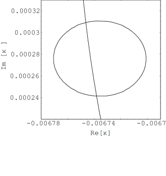
Figure 1: Contour plot on complex $\kappa$-plane in case of $\tan\beta=2.5$. The vertical line and the circle correspond to the solutions of Eqs. (9) and (10), respectively.

in the standard parameterization. By using these outputs at the GUT scale as input parameters, we solve Eqs. (9) and (10). The contours of solutions of each equations are depicted in Figure 1 for $\tan\beta=2.5$. The crossing points of two contours are the solutions. As an example, we list a solution (at the upper crossing point)

$$\kappa=-0.00675+0.000309i\;,$$

$$|c_{d}|=5.99\;,$$ (22)

for $\tan\beta=2.5$, and

$$\kappa=-0.0103+0.000606i\;,$$

$$|c_{d}|=6.32\;,$$ (23)

for $\tan\beta=10$.

Once the parameters, $|c_{d}|$ and $\kappa$, are determined, we can describe all the fermion mass matrices as a functions of $\sigma$ from the mass matrix formulas of Eqs. (6), (11) and (12). Interestingly, in the minimal $SO(10)$ model even light Majorana neutrino mass matrix, $M_{\nu}$, can be determined as a function of $\sigma$, $c_{T}$ and $c_{R}$ through the seesaw mechanism $M_{\nu}=-M_{D}^{T}M_{R}^{-1}M_{D}+M_{T}$ . The case where the the first term dominates is called type I seesaw model, while the case where the the second term dominates is called type II seesaw model. Each cases have been analyzed in detail in [10] and [11], respectively, and discussed the consistency with the current neutrino oscillation data. Recently the general case has been analyzed, it is found that the minimal $SO(10)$ model is not so good to fit all the neutrino oscillation data [12]. This means that the structure of the model is somewhat too restrictive for the neutrino sector. It would be inevitable to extend the model at least for the neutrino sector in order to make the data fitting much better. Note that there are lots of possible ways to minimally extend the model only for the neutrino sector but keep the predictive power for the charged fermion mass matrices. Remember that there are two free parameters relevant to the neutrino sector, $v_{T}$ and $v_{R}$, in the model. If $v_{T}$ is smaller than the mass scale of the neutrino oscillation data, and if $v_{R}$ is the GUT scale the resultant light neutrino mass eigenvalues through the seesaw mechanism are too small to be compatible with the scale of the neutrino oscillation data. In such a case, we have to extend the neutrino sector. For instance, we can introduce an additional ${\bf\overline{126}}$ multiplet which admits to obtain the VEV only in the $SU(2)_{L}$ triplet direction, $v_{T}^{\prime}$. Now suppose that the type II seesaw mechanism works and we obtain the light neutrino Majorana mass matrix as $Y_{126}^{\prime}v_{T}^{\prime}$, where $Y_{126}^{\prime}$ is newly introduced Yukawa coupling. If each elements in $Y_{126}^{\prime}$ are much smaller than that in $Y_{126}$, our analysis above remains correct and the predictive power for the charged fermion mass matrices is maintained. In the following analysis, we assume such a minimal extension of the model.

3 Proton decay via dimension five operator

The Yukawa interactions of the MSSM matter with the color triplet Higgs induces the following Baryon and Lepton number violating dimension five operator

$$W=C_{L}^{ijkl}Q^{i}Q^{j}Q^{k}L^{l}.$$ (24)

Here the coefficients are given by the products of the Yukawa coupling matrices and the (effective) color triplet Higgsino mass matrix, and are model dependent. In the minimal $SO(10)$ model, the coefficients are given by the products of two basic Yukawa coupling matrices, $Y_{10}$ and $Y_{126}$, and the effective $2\times 2$ color triplet Higgsino mass matrix, $M_{C}$, such as [18]

$$C_{L}^{ijkl}=\left(Y_{10}^{ij},~{}Y_{126}^{ij}\right)\left(M_{C}^{-1}\right)\left(\begin{array}[]{c}Y_{10}^{kl}\\ Y_{126}^{kl}\end{array}\right).$$ (25)

As discussed in the previous section the Yukawa coupling matrices, $Y_{10}$ and $Y_{126}$, are related to the corresponding mass matrices $M_{10}$ and $M_{126}$ such that

$$Y_{10} = \frac{c_{10}}{\alpha^{u}v\sin{\beta}}M_{10},$$

$$Y_{126} = \frac{c_{126}}{\beta^{u}v\sin{\beta}}M_{126},$$ (26)

with $v\simeq 174.1\,\mathrm{[GeV]}$. Here $\alpha^{u}$ and $\beta^{u}$ are the Higgs doublet mixing parameters introduced in the previous section, which are restricted in the range $|\alpha^{u}|^{2}+|\beta^{u}|^{2}\leq 1$. Although these parameters are irrelevant to fit the low energy experimental data of the fermion mass matrices, there are theoretical lower bound on them in order for the resultant Yukawa coupling constant not to exceed the perturbative regime. Since $c_{10}$, $c_{126}$, $M_{10}$ and $M_{126}$ are the functions of only $\sigma$, we can completely determine the Yukawa coupling matrices once $\sigma$, $\alpha^{u}$ and $\beta^{u}$ are fixed. In order to obtain the most conservative values of the proton decay rate, we make a choice of the Yukawa coupling matrices as small as possible. In the following analysis, we restrict the region of the parameters in the range $(\alpha^{u})^{2}+(\beta^{u})^{2}=1$ (we assume $\alpha^{u}$ and $\beta^{u}$ real for simplicity). Here we present examples of the Yukawa coupling matrices with fixed $\sigma=\pi$. For $\tan\beta=2.5$ with $\alpha^{u}=0.031$, we find

$$Y_{10}=\left(\begin{array}[]{ccc}\begin{array}[]{c}0.000839+2.79\times{10}^{-6}\,i\\ 0.00151-0.0000265\,i\\ 0.000692-0.000818\,i\\ \end{array}\begin{array}[]{c}0.00151-0.0000265\,i\\ 0.00479+0.0000811\,i\\ -0.0128+3.17\times{10}^{-6}\,i\end{array}\begin{array}[]{c}0.000692-0.000818\,i\\ -0.0128+3.17\times{10}^{-6}\,i\\ 0.525-0.0420\,i\end{array}\end{array}\right),$$ (27)

$$Y_{126}=\left(\begin{array}[]{ccc}\begin{array}[]{c}-0.0000613-2.17\times{10}^{-7}\,i\\ -0.000111+1.94\times{10}^{-6}\,i\\ -0.0000508+0.0000600\,i\end{array}\begin{array}[]{c}-0.000111+1.94\times{10}^{-6}\,i\\ -0.000428-2.46\times{10}^{-6}\,i\\ 0.000941-2.33\times{10}^{-7}\,i\end{array}\begin{array}[]{c}-0.0000508+0.0000600\,i\\ 0.000941-2.33\times{10}^{-7}\,i\\ 1.42\times{10}^{-7}+0.00132\,i\end{array}\end{array}\right),$$ (28)

and for $\tan\beta=10$ with $\alpha^{u}=0.111$,

$$Y_{10}=\left(\begin{array}[]{ccc}\begin{array}[]{c}0.00101+1.87\times{10}^{-6}\,i\\ 0.00179-0.0000439\,i\\ 0.000348-0.00125\,i\end{array}\begin{array}[]{c}0.00179-0.0000439\,i\\ 0.00541+0.000141\,i\\ -0.0154+5.21\times{10}^{-6}\,i\end{array}\begin{array}[]{c}0.000348-0.00125\,i\\ -0.0154+5.21\times{10}^{-6}\,i\\ 0.530-0.0567\,i\end{array}\end{array}\right),$$ (29)

$$Y_{126}=\left(\begin{array}[]{ccc}\begin{array}[]{c}-0.000244-5.21\times{10}^{-7}\,i\\ -0.000436+0.0000107\,i\\ -0.0000847+0.000305\,i\end{array}\begin{array}[]{c}-0.000436+0.0000107\,i\\ -0.00164-0.0000154\,i\\ 0.00375-1.27\times{10}^{-6}\,i\end{array}\begin{array}[]{c}-0.0000847+0.000305\,i\\ 0.00375-1.27\times{10}^{-6}\,i\\ -0.000684+0.00626\,i\end{array}\end{array}\right).$$ (30)

For the effective color triplet Higgsino mass matrix, we assume the eigenvalues being the GUT scale, $M_{G}=2\times 10^{16}\,\mathrm{[GeV]}$, which is necessary to keep the successful gauge coupling unification. Then, in general, we can parameterize the $2\times 2$ mass matrix as

$$M_{C}=M_{G}I_{2}\times U,$$ (31)

with the unitary matrix,

$$U=e^{i\varphi\sigma_{3}}\left(\begin{array}[]{cc}\begin{array}[]{c}\cos{\theta}\\ -\sin{\theta}\end{array}\begin{array}[]{c}\sin{\theta}\\ \cos{\theta}\end{array}\end{array}\right)e^{i\varphi^{\prime}\sigma_{3}}.$$ (32)

Here we omit an over all phase since it is irrelevant to calculations of the proton decay rate. Now there are five free parameters in total involved in the coefficient $C_{L}^{ijkl}$, namely, $\sigma$, $\alpha_{u}$, $\theta$, $\varphi$ and $\varphi^{\prime}$. Once these parameters are fixed, $C_{L}^{ijkl}$ is completely determined.

The proton decay mode via the dimension five operator in Eq. (24) with the Wino dressing diagram is found to be dominant, and leads to the proton decay process, $p\to K^{+}\overline{\nu}$. The decay rate for this process is approximately estimated as (in the leading order of the Cabibbo angle $\lambda\sim 0.22$)

$$\Gamma(p\to K^{+}\overline{\nu}) \simeq \Gamma(p\to K^{+}\overline{\nu_{\tau}})=\frac{m_{p}}{32\pi f_{\pi}^{2}}\,\left|\beta_{H}\right|^{2}\times\left|A_{L}A_{S}\right|^{2}\times\left(\frac{\alpha_{2}}{4\pi}\right)^{2}\frac{1}{m_{S}^{2}}$$ (33)

$$\times \Big{|}C_{L}^{2311}-C_{L}^{1312}+\lambda\left(C_{L}^{2312}-C_{L}^{1322}\right)\Big{|}^{2}$$

$$\times 5.0\times 10^{31}\,[{\mathrm{years^{-1}/GeV}}].$$

Here the first term denotes the phase factor and the hadronic factor, $\beta_{H}=0.0096\,[{\mathrm{G}eV^{3}}]$ given by lattice calculations [19]. $A_{L}\simeq 0.32$, $A_{S}\simeq 0.93$ are the long-distance and the short-distance renormalization factors about the coefficient $C_{L}^{ijkl}$, respectively. The third term in the first line comes from the Wino dressing diagram, and $m_{S}$ is a typical sparticle mass scale multiplied by the ratio of a sfermion and Wino. In the case with the mass hierarchy between the sfermions and the Wino $(\widetilde{m}_{f}\gg M_{2})$, we find $m_{S}\sim\widetilde{m}_{f}\times({\widetilde{m}_{f}}/M_{2})$. In the following numerical analysis, we take $\widetilde{m}_{f}=1\,{\mathrm{[TeV]}}$ and $M_{2}=100\,{\mathrm{[GeV]}}$.

Now we perform numerical analysis. Note that because of the very constrained flavor structure of the minimal SUSY $SO(10)$ model we can give definite predictions for the proton decay rate once the five parameters in the above are fixed. For a specific choice of the Yukawa coupling matrices in the minimal $SO(10)$ model with the type II seesaw, the proton decay rate has been calculated in [21]. In our analysis, we make no such a specific choice, and perform detailed analysis in general situations of the minimal $SO(10)$ model by varying the above five free parameters. The result for $\tan\beta=2.5$ is presented in Figure 2. Here the distributions of the proton lifetime (log years) for arbitrary choices of the five free parameters (normalized by 1) is depicted. We can see that some special sets of the free parameters can result the proton lifetime consistent with SuperK results. In that region, cancellation in the second line in Eq. (33) occurs by tuning of the free parameters in the Higgsino mass matrix. Note that number of free parameters is not enough to cancel both of the process $p\to K^{+}\overline{\nu_{\tau}}$ (dominant mode) and $p\to K^{+}\overline{\nu_{\mu}}$ (sub-dominant mode), and thus the proton lifetime has an upper bound in the $SO(10)$ model. For $\tan\beta=10$, we obtain the same figure depicted in Figure 3 but the lifetime is scaled by roughly $(2.5/10)^{2}$, which is consistent with the naive expectation that the lifetime is proportional to $1/\tan^{2}\beta$. Whole region is excluded in the case with $\tan\beta=10$.

In the case of nondegenerate masses of $M_{C}$, the parameters increase from three to $5+1$ (the last 1 is the ratio of masses). However, the results only slide by the square of this mass ratio and do not show the special cancellation.

4 Conclusion and discussions

We have discussed the minimal SUSY SO(10) model, which can reproduce the realistic charged fermion mass matrices with only one parameter left free. This model has high predictive power for the fermion Yukawa coupling matrices, and they are completely determined once a few parameters in the model fixed. This feature is essential for definite predictions of the proton decay rate vis the dimension five operators. Including additional 3 free parameters in the effective Higgsino mass matrix with mass eigenvalue being the GUT scale, we have analyzed the proton decay rate by varying the five free parameters in total. We have found that for $\tan\beta=2.5$ some special sets of the parameters predicts the proton decay rate consistent with the SuperK results, where the cancellation for the dominant modes of the proton decay amplitude occurs by tuning of the parameters. Although there exists the allowed region, it is very narrow. Our result is consistent with the one in the previous work [21] for only one specific choice of the Yukawa coupling matrices. It has been found that the resultant proton decay rate is proportional to $\tan^{2}\beta$ as expected and the allowed region eventually disappears as $\tan\beta$ becomes large, even for $\tan\beta=10$.

There are some theoretically possible ways to extend the proton lifetime. One way is to adopt a large mass hierarchy between the sfermions and the Wino as can be seen in Eq. (33). The proton lifetime is pushed up according to the squared powers of the mass hierarchy, and the allowed region becomes wide. How large the hierarchy can be depends on the mechanism of the SUSY breaking and its mediation. When we assume the minimal supergravity scenario, the cosmologically allowed region [22] consistent with the recent WMAP satellite data [23] suggests that masses between sfermion masses the Wino is not so hierarchical and the value we have taken in our analysis seems to be reasonable. Another way is to abandon the assumption of Higgsino degeneracy at the GUT scale, and to make the mass eigenvalues of the effective colored Higgsino mass matrix heavy. We can examine this possibility based on a concrete Higgs sector. However this seems to be a very difficult task even if we introduce a minimal Higgs sector in the minimal $SO(10)$ model discussed in [18] [24], since there are lots of free parameters in the Higgs sector. Furthermore, even in the minimal Higgs sector, there are lots of Higgs multiplets involved and the beta function coefficients of the gauge couplings are huge. It seems to be very hard to succeed the gauge coupling unification before blowing up of the gauge couplings. Therefore, the assumption that all the Higgs multiplets are degenerate at the GUT scale would be natural. Consequently our results show the typical properties of SO(10) GUT but are not exhaustive. Also there is possibility to vary GUT phases $\alpha$, $\beta$, $\gamma$, $\beta^{\prime}$ and $\gamma^{\prime}$ in Eq. (13).

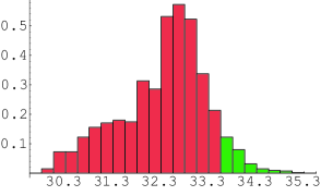
Figure 2: The distributions of the proton lifetime (log years) for $\tan\beta=2.5$ in arbitrary five parameter choices (normalized by 1). The green region (right hand side) is consistent with experiment.

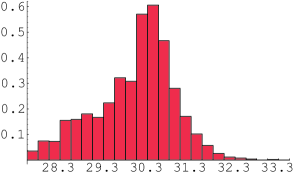
Figure 3: Same as in Figure 2, but for $\tan\beta=10$.

References

- [1] H. Georgi and S.L. Glashow, Phys. Rev. Lett. 32, 438 (1974).
- [2] U. Amaldi, W.de Boer, and H. Fürstenau, Phys. Lett. B260, 447 (1991); P. Langacker and M. Luo, Phys. Rev. D44, 817 (1991).
- [3] M. Shiozawa, talk at the 4th workshop on ”Neutrino Oscillations and their Origin” (NOON 2003), [http://www-sk.icrr.u-tokyo.ac.jp/noon2003/].
- [4] H. Murayama and A. Pierce, Phys. Rev. D65, 055009 (2002).
- [5] T. Goto and T. Nihei, Phys. Rev. D59, 115009 (1999).
- [6] B. Bajc, P.F. Perez and G. Senjanovic, Phys. Rev. D66, 075005 (2002).
- [7] D. Emmanuel-Costa and S. Wiesenfeldt, Nucl. Phys. B 661, 62 (2003)
- [8] T. Yanagida, in Proceedings of the workshop on the Unified Theory and Baryon Number in the Universe, edited by O. Sawada and A. Sugamoto (KEK, Tsukuba, 1979); M. Gell-Mann, P. Ramond, and R. Slansky, in Supergravity, edited by D. Freedman and P. van Nieuwenhuizen (North-Holland, Amsterdam, 1979); R.N. Mohapatra and G. Senjanovic, Phys. Rev. Lett. 44, 912 (1980).
- [9] K.S. Babu and R.N. Mohapatra, Phys. Rev. Lett. 70, 2845 (1993).
- [10] T. Fukuyama and N. Okada, JHEP 0211, 011 (2002); K. Matsuda, Y. Koide, T. Fukuyama and H. Nishiura, Phys. Rev. D65, 033008 (2002) [Erratum-ibid. D65, 079904 (2002)]; K. Matsuda, Y. Koide and T. Fukuyama, Phys. Rev. D64, 053015 (2001).
- [11] B. Bajc, G. Senjanovic and F. Vissani, Phys. Rev. Lett. 90, 051802 (2003); H.S. Goh, R.N. Mohapatra and Siew-Phang Ng, Phys. Lett. B570, 215 (2003), Phys. Rev. D68, 115008 (2003).
- [12] B. Dutta, Y. Mimura and R.N. Mohapatra, arXiv: hep-ph/0402113.
- [13] P.F. Perez, arXiv: hep-ph/0403286.
- [14] J.C. Pati and A. Salam, Phys. Rev. D10, 275 (1974).
- [15] H. Fusaoka and Y. Koide, Phys. Rev. D57, 3986 (1998).
- [16] K. Hagiwara et al. [Particle Data Group Collaboration], Phys. Rev. D66, 010001 (2002).
- [17] LEP Higgs Working Group and ALEPH collaboration and DELPHI collaboration and L3 collaboration and OPAL Collaboration, arXiv: hep-ex/0107030.
- [18] T. Fukuyama, A. Ilakovac, T. Kikuchi, S. Meljanac, and N. Okada, arXiv: hep-ph/0401213.
- [19] N. Tsutsui et al. [CP-PACS collabolation and JLQCD collaboration], [arXiv:hep-lat/0402026].
- [20] K. Turzynski, JHEP 0210, 044 (2002).
- [21] H.S. Goh, R.N. Mohapatra, S. Nasri, Siew-Phang Ng, Phys. Lett. B587, 105 (2004).
- [22] For a review article, for example, A.B. Lahanas, N.E. Mavromatos, D.V. Nanopoulos, Int. J. Mod. Phys. D12 1529, (2003).
- [23] C.L. Bennett et al., Astrophys. J. Suppl. 148, 1 (2003); D.N. Spergel et al., Astrophys. J. Suppl. 148, 175 (2003).
- [24] B. Bajc, A. Melfo, G. Senjanovic and F. Vissani, arXiv:hep-ph/0402122.