Status of Global Analysis of Neutrino Oscillation Data

Abstract

In this talk we discuss some details of the analysis of neutrino data and our present understanding of neutrino masses and mixing. This talk is based on Refs. [newthree,ourcpt,atmnp].

1 Analysis of Solar and KamLAND

In Fig. 1 we show the results from our latest analysis of KamLAND [kland] reactor $\overline{\nu}_{e}$ disappearance data, solar $\nu_{e}$ data [sksol,sno2] and the combined analysis under the hypothesis of CPT symmetry. The main new ingredient in this analysis with respect to the previous ones is the inclusion of the first results from the SNO salt phase (SNOII) data [sno2]. We have also taken into account the new gallium measurement which leads to the new average value $69.3\pm 4.0$. The main changes as compared to the pre-SNOII analysis are:

• in the analysis of solar data, only LMA is allowed at more than $3\sigma$;

• maximal mixing is rejected by the solar analysis at more than $5\sigma$;

• the combined analysis allows only the lowest LMA region at 99.4% CL;

• the new best-fit point is:

  $$\Delta m^{2}=7.1\times 10^{-5}~{}\text{eV}^{2}\,,\qquad\tan^{2}\theta=0.41\,,\qquad\frac{\Phi_{\rm{}^{8}B}}{\Phi_{\rm{}^{8}B,BP04}}=0.88\,.$$ (1)

These results are in agreement with those reported in the several state-of-the-art analysis of solar and KamLAND data which exist in the literature. All these analysis share the same basic characteristics.

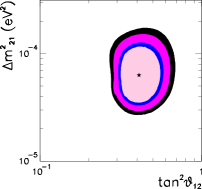
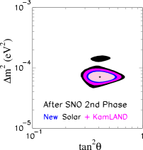
Figure 1: Allowed regions for 2-$\nu$ oscillations of $\bar{\nu}_{e}$ in KamLAND and CHOOZ (left panel), of $\nu_{e}$ in the sun (central panel), and for the combination of KamLAND and solar data under the hypothesis of CPT conservation (right). The different contours correspond to the allowed regions at 90%, 95%, 99% and $3\sigma$ CL.

In the analysis of KamLAND we used the following approximations:

• the antineutrino spectrum is parameterized [vogel] without detailed theoretical uncertainties;

• the yearly average reactor power is used.

Presently the uncertainties of the KamLAND results are statistics dominated so these effects do not make any difference in the extracted allowed regions. The minor differences between the several phenomenological analysis in the literature are more likely to arise from the use of different statistical functions in the analysis of KamLAND data.

Before moving to atmospheric neutrinos, we wish to point out some important features of the analysis of solar data:

• the SSM [carlos] provides detailed informations not only on the solar neutrino fluxes themselves, but also on their theoretical uncertainties and correlations due to variations of the SSM inputs;

• the spectral shape experimental uncertainty for ⁸B spectrum is properly taken into account;

• the energy dependence of the interaction cross sections and their uncertainties is also included;

• the interplay between the energy-dependent part of the theoretical and systematic uncertainties and the neutrino survival probability (which depends on the oscillation parameters) is properly taken into account.

2 Atmospheric Neutrinos

In the left panel of Fig. 2 we show the results of our latest analysis of the atmospheric neutrino data, which included the full data set of Super-Kamiokande phase I (SK1). As discussed in Ref. [skatmos] the new elements in the Super-Kamiokande analysis include:

• use of new three-dimensional fluxes from Honda [honda3d];

• improved interaction cross sections which agree better with the measurements performed with near detector in K2K [k2k];

• some improvements in the Monte-Carlo which lead to some changes in the actual values of the data points.

We have included these elements in our calculations and we have also improved our statistical analysis (see Ref. [atmnp] for details). Our results show good quantitative agreement with those of the Super-K collaboration. In particular we find that after inclusion of the above effects, the allowed region is shifted to lower $\Delta m^{2}$. The new best-fit point is located at:

$$\Delta m^{2}=2.2\times 10^{-3}~{}\text{eV}^{2}\,,\qquad\sin^{2}\theta=0.5\,.$$ (2)

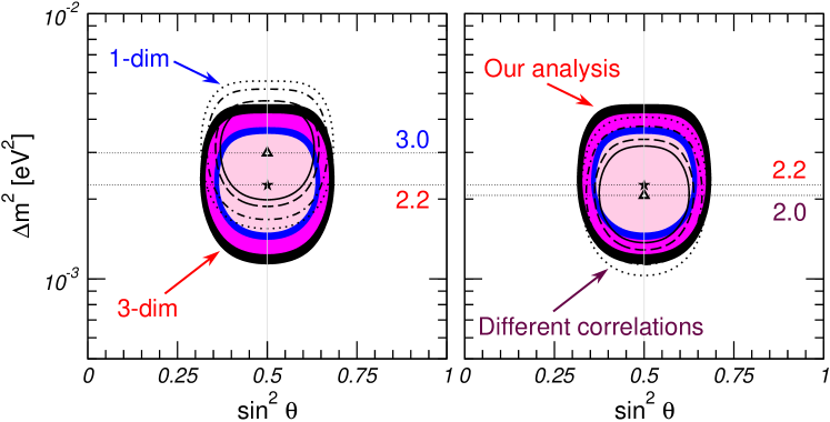
Figure 2: Left: allowed regions from the analysis of atmospheric data using the new (full regions labeled “3-dim”) and old (empty curves labeled as “1-dim”) SK1 data and atmospheric fluxes. Right: impact of a small change in the correlation between the theoretical uncertainties of the low-energy (sub-GeV) and high-energy (multi-GeV, and upgoing $\mu$) data samples. The different contours correspond to at 90%, 95%, 99% and $3\sigma$ CL.

At this point it is important to remark that, unlike for solar neutrinos, the energy dependence of the theoretical uncertainties in the atmospheric fluxes and in the interaction cross sections are not so well determined in terms of a set of model inputs. To address this issue, we have performed the same analysis assuming slightly different correlations among the theoretical errors for the different data sets, and we have found that the size of the final shift in $\Delta m^{2}$ of the allowed region depends on these details (see right panel of Fig. 2). The reason for this behavior is illustrated in Fig. 3, where we show the allowed regions obtained with the new analysis as compared to the old one for the different atmospheric data sets. As can be seen in the figure, the different sets favor slightly different ranges of $\Delta m^{2}$, thus the treatment of the energy dependence of the uncertainties becomes relevant in outcome of the combined analysis.

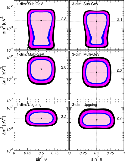
Figure 3: The left (right) panels show the allowed regions for the analysis of the different sets of atmospheric data using the new (old) SK1 analysis and atmospheric fluxes. The different contours correspond to the allowed regions at 90%, 95%, 99% and $3\sigma$ CL.

These results lead us to raise here a word of caution. In all present analysis of atmospheric data, two main sources of theoretical flux uncertainties are included: an energy independent normalization error and a “tilt” error which parametrizes the uncertainty in the $E^{-\gamma}$ dependence of the flux. Some additional uncertainties in the ratios of the samples at different energies are also allowed as well as uncertainties in the zenith dependences. However, we still lack a well established range of theoretical flux uncertainties within a given atmospheric flux calculation, in a similar fashion to what it is provided for the solar neutrino fluxes by the SSM. In the absence of these, we cannot be sure that we are accounting for the most general characterization of the energy dependence of the atmospheric neutrino flux uncertainties.

Given the large amount of data points provided by the Super-K experiment, this is becoming an important issue in the atmospheric neutrino analysis. There is a chance that the atmospheric fluxes may be still too “rigid”, even when allowed to change within the presently considered uncertainties. As a consequence, we may be over-constraining the oscillation parameters.

3 Three-Neutrino Oscillations

The minimum joint description of atmospheric [skatmos], K2K [k2k], solar [sksol,sno2] and reactor [kland,chooz] data requires that all the three known neutrinos take part in the oscillation process. The mixing parameters are encoded in the $3\times 3$ lepton mixing matrix which can be conveniently parametrized in the standard form:

$$U=\left(\begin{array}[]{ccc}1&0&0\\ 0&{c_{23}}&{s_{23}}\\ 0&-{s_{23}}&{c_{23}}\end{array}\right)\times\left(\begin{array}[]{ccc}{c_{13}}&0&{s_{13}}e^{i{\delta}}\\ 0&1&0\\ -{s_{13}}e^{-i{\delta}}&0&{c_{13}}\end{array}\right)\times\left(\begin{array}[]{ccc}c_{21}&{s_{12}}&0\\ -{s_{12}}&{c_{12}}&0\\ 0&0&1\end{array}\right)$$ (3)

where $c_{ij}\equiv\cos\theta_{ij}$ and $s_{ij}\equiv\sin\theta_{ij}$. Note that the two Majorana phases are not included in the expression above since they do not affect neutrino oscillations. The angles $\theta_{ij}$ can be taken without loss of generality to lie in the first quadrant, $\theta_{ij}\in[0,\pi/2]$.

There are two possible mass orderings, which we denote as “normal” and “inverted”. In the normal scheme $m_{1}<m_{2}<m_{3}$ while in the inverted one $m_{3}<m_{1}<m_{2}$. The two orderings are often referred to in terms of $\mathop{\rm sign}\nolimits(\Delta m^{2}_{31})$.

In total the three-neutrino oscillation analysis involves seven parameters: 2 mass differences, 3 mixing angles, the CP phase and the sign of $\Delta m^{2}_{31}$. Generic three-neutrino oscillation effects include:

• coupled oscillations with two different oscillation lengths;

• CP violating effects;

• difference between Normal and Inverted schemes.

The strength of these effects is controlled by the values of the ratio of mass differences $\alpha\equiv\Delta m^{2}_{21}/|\Delta m_{31}^{2}|$, by the mixing angle $\theta_{13}$ and by the CP phase $\delta$.

For solar and atmospheric oscillations, the required mass differences satisfy:

$$\Delta m^{2}_{\odot}=\Delta m^{2}_{21}\ll|\Delta m_{31}^{2}|=\Delta m^{2}_{\rm atm}.$$ (4)

Under this condition, the joint three-neutrino analysis simplifies and we have:

• for solar and KamLAND neutrinos, the oscillations with the atmospheric oscillation length are completely averaged and the survival probability takes the form:

  $$P^{3\nu}_{ee}=\sin^{4}\theta_{13}+\cos^{4}\theta_{13}P^{2\nu}_{ee}$$ (5)

  where in the Sun $P^{2\nu}_{ee}$ is obtained with the modified sun density $N_{e}\rightarrow\cos^{2}\theta_{13}N_{e}$. So the analyses of solar data constrain three of the seven parameters: $\Delta m^{2}_{21},\theta_{12}$ and $\theta_{13}$. The effect of $\theta_{13}$ is to decrease the energy dependence of the solar survival probability;

• for atmospheric and K2K neutrinos, the solar wavelength is too long and the corresponding oscillating phase is negligible. As a consequence, the atmospheric data analysis restricts $\Delta m^{2}_{31}\simeq\Delta m^{2}_{32}$, $\theta_{23}$ and $\theta_{13}$, the latter being the only parameter common to both solar and atmospheric neutrino oscillations and which may potentially allow for some mutual influence. The effect of $\theta_{13}$ is to add a $\nu_{\mu}\rightarrow\nu_{e}$ contribution to the atmospheric oscillations;

• at CHOOZ [chooz] the solar wavelength is unobservable if $\Delta m^{2}<8\times 10^{-4}~{}\text{eV}^{2}$ and the relevant survival probability oscillates with wavelength determined by $\Delta m^{2}_{31}$ and amplitude determined by $\theta_{13}$.

In this approximation, the CP phase is unobservable. In principle there is a dependence on the Normal versus Inverted orderings due to matter effects in the Earth for atmospheric neutrinos. However, this effect is controlled by the mixing angle $\theta_{13}$, which is constrained to be small by the combined analysis of CHOOZ reactor and atmospheric analysis. As a consequence, this effect is too small to be statistically meaningful in the present analysis.

In Fig. 4 we plot the individual bounds on each of the five parameters derived from the global analysis. To illustrate the impact of SNOII and the new ATM analysis we also show the corresponding bounds when either SNOII and the new ATM fluxes are not included in the analysis. In each panel the displayed $\chi^{2}$ has been marginalized with respect to the undisplayed parameters.

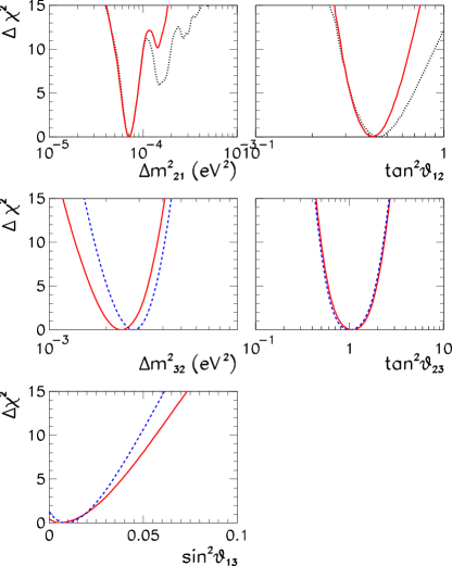
Figure 4: Global $3\nu$ oscillation analysis. Each panel on the left shows the dependence of $\Delta\chi^{2}$ on each of the five parameters from the global analysis (full line) compared to the bound prior to the inclusion of the new ATM analysis (dashed blue line) and SNO data (dotted black line).

Quantitatively we find the following $3\sigma$ CL allowed ranges:

$$5.2\leq\Delta m^{2}_{21}/{10^{-5}~{}\text{eV}^{2}} \leq 9.8\,, \quad 0.29\leq\tan^{2}\theta_{12} \leq 0.64\,,$$

$$1.4\leq\Delta m^{2}_{32}/{10^{-3}~{}\text{eV}^{2}} \leq 3.4\,, \quad 0.49\leq\tan^{2}\theta_{23} \leq 2.2\,,$$ (6)

$$\sin^{2}\theta_{13} \leq 0.054\,.$$

These results can be translated into our present knowledge of the moduli of the mixing matrix $U$:

$$|U|=\left(\begin{array}[]{ccc}0.78-0.88&0.47-0.62&<0.23\\ 0.18-0.55&0.40-0.73&0.57-0.82\\ 0.19-0.55&0.41-0.75&0.55-0.82\end{array}\right)$$ (7)

which presents a structure

$$|U|\simeq\left(\begin{array}[]{ccc}\frac{1}{\sqrt{2}}(1+{\lambda})&\frac{1}{\sqrt{2}}(1-{\lambda})&{\epsilon}\\ \frac{1}{{2}}(1-{\lambda}+{\Delta}+{\epsilon}\,{\cos\delta})&\frac{1}{{2}}(1+{\lambda}+{\Delta}-{\epsilon}\,{\cos\delta})&\frac{1}{\sqrt{2}}(1-{\Delta})\\ \frac{1}{{2}}(1-{\lambda}-{\Delta}-{\epsilon}\,{\cos\delta})&\frac{1}{{2}}(1+{\lambda}-{\Delta}+{\epsilon}\,{\cos\delta})&\frac{1}{\sqrt{2}}(1+{\Delta})\end{array}\right)$$ (8)

with $1\sigma$ ranges

$$\lambda=0.23\pm 0.03\,,\quad\Delta=0\pm 0.08\,,\quad\epsilon\leq 0.02\,,\quad-1\leq\cos\delta\leq 1\,.$$ (9)

3.1 LSND and Sterile Neutrinos

Together with the results from the solar and atmospheric neutrino experiments, we have one more piece of evidence pointing towards the existence of neutrino masses and mixing: the LSND experiment, which found evidence of $\overline{\nu}_{\mu}\rightarrow\overline{\nu}_{e}$ neutrino conversion with $\Delta m^{2}\geq 0.1~{}\text{eV}^{2}$. All these data can be accommodated into a single neutrino oscillation framework only if there are at least three different scales of neutrino mass-squared differences. This requires the existence of a fourth light neutrino, which must be sterile in order not to affect the invisible $Z^{0}$ decay width, precisely measured at LEP.

One of the most important issues in the context of four-neutrino scenarios is the neutrino mass spectrum. There are six possible four-neutrino schemes which can in principle accommodate the results of solar and atmospheric neutrino experiments as well as the LSND result. They can be divided in two classes: (3+1) and (2+2). In the (3+1) schemes, there is a group of three close-by neutrino masses that is separated from the fourth one by a gap of the order of 1 $\text{eV}^{2}$, which is responsible for the SBL oscillations observed in the LSND experiment. In (2+2) schemes, there are two pairs of close masses separated by the LSND gap. The main difference between these two classes is the following: if a (2+2)-spectrum is realized in nature, the transition into the sterile neutrino is a solution of either the solar or the atmospheric neutrino problem, or the sterile neutrino takes part in both. This is not the case for a (3+1)-spectrum, where the sterile neutrino could be only slightly mixed with the active ones and mainly provide a description of the LSND result.

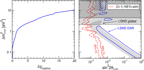
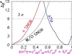
Figure 5: Left: Status of the 3+1 oscillation scenarios. Right: Present status of the bounds on the active-sterile admixture from solar and atmospheric neutrino data in (2+2)-models.

The phenomenological situation at present is that none of the four-neutrino scenarios are favored by the data. Concerning (2+2)-spectra, they are ruled out by the existing constraints from the sterile oscillations in solar and atmospheric data. As for (3+1)-spectra, they are disfavored by the incompatibility between the LSND signal and and the negative results found by other short-baseline laboratory experiments. There is also a constraint on the possible value of the heavier neutrino mass in this scenario from their contribution to the energy density in the Universe which is presently constrained by cosmic microwave background radiation and large scale structure formation data [cosmo].

We show in Fig. 5 the latest results of the analysis of neutrino data in these scenarios. In the left and central panel we summarize the results from Ref. [michele] on the (3+1) scenarios; we see that after the inclusion of the cosmological bound there is only a marginal overlap at 95% CL between the allowed LSND region and the excluded region from SBL+ATM experiments. The right panel illustrates the status of the (2+2) scenarios. At present, the lower bound on the sterile component from the analysis of atmospheric data and the upper bound from the analysis of solar data do not overlap at more than $4\sigma$. The figure also illustrates the effect of the inclusion of the SNOII in this conclusion.

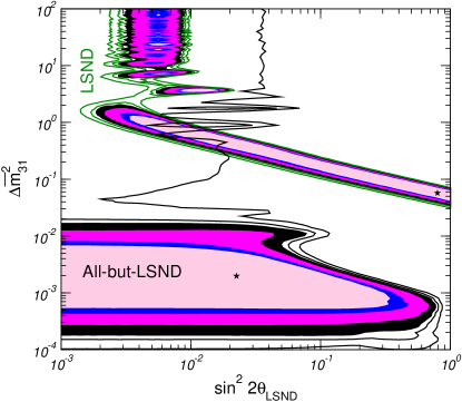
Figure 6: 90%, 95%, 99%, and $3\sigma$ CL allowed regions (filled) in required to explain the LSND signal together with the corresponding allowed regions from our global analysis of all-but-LSND data. The contour lines correspond to $\Delta\chi^{2}=13$ and 16 (3.2$\sigma$ and 3.6$\sigma$, respectively).

Alternative explanations to the LSND result include the possibility of CPT violation [CPT], which implies that the masses and mixing angles of neutrinos may be different from those of antineutrinos. We have performed an analysis of the existing data from solar, atmospheric, long baseline, reactor and short baseline data in the framework of CPT violating oscillations [ourcpt]. The summary of the results of this analysis is presented in Fig. 6, which shows clearly that there is no overlap below the $3\sigma$ level between the LSND and the all-but-LSND allowed regions. We also note that that the all-but-LSND region is restricted to $\Delta\overline{m}_{31}^{2}=\Delta m^{2}_{\rm LSND}<0.02~{}\text{eV}^{2}$, whereas for LSND we always have $\Delta\overline{m}_{31}^{2}=\Delta m^{2}_{\rm LSND}>0.02~{}\text{eV}^{2}$.

References

- [1] M. C. Gonzalez-Garcia and C. Pena-Garay, Phys. Rev. D 68, 093003 (2003).
- [2] M. C. Gonzalez-Garcia, M. Maltoni and T. Schwetz, Phys. Rev. D 68, 053007 (2003).
- [3] M. C. Gonzalez-Garcia and M. Maltoni, hep-ph/0404085.
- [4] See S. Freedman in these proceedings.
- [5] See Y. Koshio in these proceedings.
- [6] See K. Graham in these proceedings.
- [7] See C. Peña-Garay in these proceedings.
- [8] P. Vogel and J. Engel, Phys. Rev. D 39, 3378 (1989).
- [9] See C. Saji in these proceedings.
- [10] M. Honda, T. Kajita, K. Kasahara and S. Midorikawa, astro-ph/0404457.
- [11] See T. Ishii in these proceedings.
- [12] M. Apollonio et al., Phys. Lett. B 466 (1999) 415.
- [13] M. Maltoni, T. Schwetz, M. A. Tortola and J. W. F. Valle, Nucl. Phys. B 643, 321 (2002); see also hep-ph/0305312.
- [14] See M. Kawasaki in these proceedings.
- [15] H. Murayama, and T. Yanagida, Phys. Lett. B 520, 263 (2001); G. Barenboim et al., JHEP 0210 (2002) 001, hep-ph/0108199.