CP asymmetry, branching ratios, and isospin breaking effects of $B\to K^{*}\gamma$ with the perturbative QCD approach

Abstract

The main contribution to the radiative ${B\rightarrow K^{*}\gamma}$ mode is from penguin operators which are quantum corrections. Thus, this mode may be useful in the search for physics beyond the standard model. In this paper, we compute the branching ratio, direct CP asymmetry, and isospin breaking effects within the standard model in the framework of perturbative QCD, and discuss how new physics might show up in this decay.

I Introduction

The large CP violation in ${B\rightarrow J/\psi K_{s}}$ decay mode predicted by the standard model with Kobayashi-Masukawa (KM) scheme has been verified by ${B}$ factories at KEK ( High Energy Accelerator Research Organization) and Stanford Linear Accelerator Center (SLAC). The standard model predicts the CP asymmetries for ${B\rightarrow J/\psi K_{s}}$ and ${B\rightarrow\phi K_{s}}$ to be equal to ${\sin{2\phi_{1}}}$. However, recent experimental data from Belle showed that these asymmetries differ by nearly ${2\sigma}$; the averaged ${\sin{2\phi_{1}}}$ from Bell and BaBar in ${B\to J/\psi K_{s}}$ system is ${\sin{2\phi_{1}}=0.736\pm 0.049}$ Eidelman:2004wy and in ${B\rightarrow\phi K_{s}}$ decay mode is ${\sin{2\phi_{1}}=0.06\pm 0.33\pm 0.09}$ from Belle Abe:2004xp , and ${\sin{2\phi_{1}}=0.50\pm 0.25^{+0.07}_{-0.04}}$ from BaBar Aubert:2004dy . Experimental error is still large, so the situation is inconclusive, but if this result continues to hold, it implies existence of new physics beyond the standard model.

In this paper, we want to concentrate on ${B\rightarrow K^{*}\gamma}$ decay mode. The decay mode has large a branching ratio, so the experimental error on the CP asymmetry has been getting small and is now down to several percent.

$$Br(B^{0}\rightarrow K^{*0}\gamma)=\begin{cases}(4.01\pm 0.21\pm 0.17)\times 10^{-5}&\mbox{\cite[cite]{\@@bibref{Authors Phrase1YearPhrase2}{Nakao:2004th}{\@@citephrase{(}}{\@@citephrase{)}}}}\\ (3.92\pm 0.20\pm 0.24)\times 10^{-5}&\mbox{\cite[cite]{\@@bibref{Authors Phrase1YearPhrase2}{Aubert:2004te}{\@@citephrase{(}}{\@@citephrase{)}}}}\end{cases}$$

$$Br(B^{\pm}\rightarrow K^{*\pm}\gamma)=\begin{cases}(4.25\pm 0.31\pm 0.24)\times 10^{-5}&\mbox{\cite[cite]{\@@bibref{Authors Phrase1YearPhrase2}{Nakao:2004th}{\@@citephrase{(}}{\@@citephrase{)}}}}\\ (3.87\pm 0.28\pm 0.26)\times 10^{-5}&\mbox{\cite[cite]{\@@bibref{Authors Phrase1YearPhrase2}{Aubert:2004te}{\@@citephrase{(}}{\@@citephrase{)}}}}\end{cases}$$

$$A_{CP}=\begin{cases}-0.015\pm 0.044\pm 0.012&\mbox{\cite[cite]{\@@bibref{Authors Phrase1YearPhrase2}{Nakao:2004th}{\@@citephrase{(}}{\@@citephrase{)}}}}\\ -0.013\pm 0.036\pm 0.010&\mbox{\cite[cite]{\@@bibref{Authors Phrase1YearPhrase2}{Aubert:2004te}{\@@citephrase{(}}{\@@citephrase{)}}}}\end{cases}$$

CP Asymmetry is defined as

$$A_{CP}\equiv\frac{\Gamma(\bar{B}\to\bar{K^{*}}\gamma)-\Gamma(B\to K^{*}\gamma)}{\Gamma(\bar{B}\to\bar{K^{*}}\gamma)+\Gamma(B\to K^{*}\gamma)}~{},$$ (1)

and in general, theoretical predictions of the CP asymmetries depend less on hadronic parameters than those of branching ratios as many uncertainties cancel in the ratio. So comparing predictions for CP asymmetries within the standard model with experimental data may be effective way to search for new physics. Many authors have pointed out for some time, that the CP asymmetry in this mode is very small. We can easily understand why the asymmetry is so small. In order to generate CP asymmetry, at least two amplitudes with nonvanishing relative weak and strong phases must interfere. This decay is mainly caused by an ${O_{7\gamma}}$ operator, and other contributions which interfere with this contribution are small and the Cabibbo-Kobayashi-Masukawa quark-mixing matrix (CKM) unitary triangle is crushed, making the CP asymmetry in this decay mode very small. However, if we were to look for new physics, we need to be able to give a quantitative estimate of the standard model contribution to the CP asymmetry. For this purpose, we include small contributions which interfere with ${O_{7\gamma}}$, including also the long distance contributions, for example, ${B\rightarrow K^{*}J/\psi\rightarrow K^{*}\gamma}$.

Furthermore, the isospin breaking effect ${\Delta_{0+}}$ is also very interesting because it’s size and sign are sensitive to the existence of physics beyond the standard model.

$$\Delta_{0+} \equiv \frac{\Gamma(B^{0}\to K^{*0}\gamma)-\Gamma(B^{+}\to K^{*+}\gamma)}{\Gamma(B^{0}\to K^{*0}\gamma)+\Gamma(B^{+}\to K^{*+}\gamma)}$$

$$= \frac{(\tau_{B^{+}}/\tau_{B^{0}})Br(B^{0}\to K^{*0}\gamma)-Br(B^{+}\to K^{*+}\gamma)}{(\tau_{B^{+}}/\tau_{B^{0}})Br(B^{0}\to K^{*0}\gamma)+Br(B^{+}\to K^{*+}\gamma)}$$

In order to test the standard model, we need to know if the penguin contribution within the standard model can explain the experimental data. Experiments show ${\Delta_{0+}=+0.012\pm 0.044\pm 0.026}$ in Bell Nakao:2004th and ${\Delta_{0-}=0.050\pm 0.045\pm 0.028\pm 0.024}$ in BaBar Aubert:2004te . More precise data will become available in the near future, so the theoretical prediction of it’s size and sign of this asymmetry should be pinned down.

In this paper, we calculate the branching ratio, direct CP asymmetry, and isospin breaking effects in ${B\to K^{*}\gamma}$ decay mode, based on the standard model. First, we briefly review the concept of the pQCD in Sect.II, and in Sect.III, we show the effective Hamiltonian which causes ${B\to K^{*}\gamma}$ decay. Then we present the factorization formulas for the ${B\rightarrow K^{*}\gamma}$ decay mode in Sect.IV, and in Sect.V, we mention about the long distance contributions. Next we will show the numerical results in Sect.VI, and Sect.VII is our conclusion. Finally in Appendix A, we present a brief review of pQCD.

II Outline of pQCD

Theoretically, it is easy to analyze the inclusive ${B}$ meson decay like ${B\rightarrow X_{s}\gamma}$ because we can estimate the decay width, for example, by inserting the complete set for all possible intermediate states. The experimental and theoretical branching ratio of ${B\to X_{s}\gamma}$ are

$$Br(B\to X_{s}\gamma)^{\scriptsize\mbox{exp}} = (3.52^{+0.30}_{-0.28})\times 10^{-4},\hskip 14.22636pt\mbox{\cite[cite]{\@@bibref{Authors Phrase1YearPhrase2}{Alexander:2005cx}{\@@citephrase{(}}{\@@citephrase{)}}}}$$

$$Br(B\to X_{s}\gamma)^{\scriptsize\mbox{th}} = (3.57\pm 0.30)\times 10^{-4},\hskip 14.22636pt\mbox{\cite[cite]{\@@bibref{Authors Phrase1YearPhrase2}{Buras:2002tp}{\@@citephrase{(}}{\@@citephrase{)}}}}$$

and this good agreement strongly constraints new physics parameters. However, inclusive decays are experimentally difficult to analyze because all ${B\to X_{s}\gamma}$ candidates should be counted. If we can directly calculate the exclusive decay mode ${B\to K^{*}\gamma}$, we ought to obtain many interesting results to test the standard model or to search for new physics.

Perturbative QCD is one of the theoretical instrument for handling the exclusive decay modes. The concept of pQCD is the factorization between soft and hard dynamics. In order to physically understand the pQCD approach, we consider ${B^{0}}$ meson decays into ${K^{*0}}$ meson and ${\gamma}$ in the rest frame of the ${B^{0}}$ meson (Fig.1). The heavy ${\bar{b}}$ quark which has most of ${B^{0}}$ meson mass is nearly static in this frame and the other quark, which forms the ${B^{0}}$ meson together with the ${\bar{b}}$ quark, called the spectator quark, carries momentum of order ${O(\bar{\Lambda})=O(M_{B}-m_{b})}$. This ${\bar{b}}$ quark decays into the light ${\bar{s}}$ quark and ${\gamma}$ through the electromagnetic penguin operator and the decay products dash away back-to-back, with momentum of ${O(M_{B}/2)}$. (This process is depicted in Fig.1(a).) ${K^{*0}}$ meson is composed of ${\bar{s}}$ quark and a spectator quark. In order for the fast moving ${\bar{s}}$ quark and slow moving spectator ${d}$ quark to form a ${K^{*0}}$ meson and nothing else, the spectator quark must be kicked by the gluon, so that the ${\bar{s}}$ and ${d}$ quark have more or less parallel momenta in the direction of ${K^{*0}}$. (This process is depicted in Fig.1(b).) Since the invariant-mass square of this gluon is the order of ${O(\bar{\Lambda}M_{B})}$, we can treat this decay process perturbatively.

(a)                                         (b)

Figure 1: The left figure is no gluon exchange diagram. ${\bar{s}}$ and spectator ${d}$ are not lines up to form an energetic ${K^{*}}$ meson. In order to hadronize ${K^{*}}$ meson, one gluon with large ${q^{2}}$ should be exchanged.

There is also diagram shown in Fig.2. This can also be computed in the pQCD approach. The diagram can be cut along the dotted line indicating the presence of the physical intermediate state. This results in a strong interaction phase which can be computed. The direct CP asymmetry is caused by interfering some amplitudes which have relative weak and strong phase, and it can be written in the form proportioning to ${\sin{(\theta_{w1}-\theta_{w2})}\sin{(\delta_{s1}-\delta_{s2})}}$: in short, it depends on both weak and strong phases.

$$A(B\to f) = A_{1}e^{i\theta_{w1}}e^{i\delta_{s1}}+A_{2}e^{i\theta_{w2}}e^{i\delta_{s2}}$$

$$A(\bar{B}\to\bar{f}) = A_{1}e^{-i\theta_{w1}}e^{i\delta_{s1}}+A_{2}e^{-i\theta_{w2}}e^{i\delta_{s2}}$$

We can determine the strong phases by using the pQCD approach, then we can extract the information about the weak phases and examine the standard model. A more detailed review for the pQCD approach is in Appendix A.

Figure 2: Example of annihilation diagram which produces strong phase through the branch-cut.

III Kinematics for ${B\rightarrow K^{*}\gamma}$ decay mode

The effective Hamiltonian which induces flavor-changing ${b\rightarrow s\gamma}$ transition is given by Buchalla:1995vs

$$H_{eff} = \frac{G_{F}}{\sqrt{2}}\Big{[}\sum_{q=u,c}V_{qb}V_{qs}^{*}\left(C_{1}(\mu)O_{1}^{(q)}(\mu)+C_{2}(\mu)O_{2}^{(q)}(\mu)\right)$$ (3)

$$\hskip 28.45274pt-V_{tb}V_{ts}^{*}\sum_{i=3\sim 8g}C_{i}(\mu)O_{i}(\mu)\Big{]}+\mbox{h.c.}~{},$$

$$O_{1}^{(q)}=(\bar{s}_{i}q_{j})_{V-A}(\bar{q}_{j}b_{i})_{V-A},$$

$$O_{2}^{(q)}=(\bar{s}_{i}q_{i})_{V-A}(\bar{q}_{j}b_{j})_{V-A},$$

$$O_{3}=(\bar{s}_{i}b_{i})_{V-A}\sum_{q}(\bar{q}_{j}q_{j})_{V-A},$$

$$O_{4}=(\bar{s}_{i}b_{j})_{V-A}\sum_{q}(\bar{q}_{j}q_{i})_{V-A},$$ (4)

$$O_{5}=(\bar{s}_{i}b_{i})_{V-A}\sum_{q}(\bar{q}_{j}q_{j})_{V+A},$$

$$O_{6}=(\bar{s}_{i}b_{j})_{V-A}\sum_{q}(\bar{q}_{j}q_{i})_{V+A},$$

$$O_{7\gamma}=\frac{e}{4{\pi}^{2}}\bar{s}_{i}\sigma^{\mu\nu}(m_{s}P_{L}+m_{b}P_{R})b_{i}F_{\mu\nu},$$

$$O_{8g}=\frac{g}{4{\pi}^{2}}\bar{s}_{i}\sigma^{\mu\nu}(m_{s}P_{L}+m_{b}P_{R})T_{ij}^{a}b_{j}G_{\mu\nu}^{a},$$

where ${P^{L}_{R}=(1\mp\gamma^{5})/2}$. We define the ${B}$ meson and the ${K^{*}}$ meson momenta ${P_{1}}$ and ${P_{2}}$ in the light-cone coordinates

$$p=(p^{+},p^{-},\vec{p}_{T})=\left(\frac{p^{0}+p^{3}}{\sqrt{2}},\frac{p^{0}-p^{3}}{\sqrt{2}},(p^{1},p^{2})\right)$$ (5)

within the ${B}$ meson rest frame as

$$P_{1} = (P_{1}^{+},P_{1}^{-},\vec{P}_{1T})=\frac{M_{B}}{\sqrt{2}}(1,1,\vec{0}_{T}),$$ (6)

$$P_{2} = (P_{2}^{+},P_{2}^{-},\vec{P}_{2T})=\frac{M_{B}}{\sqrt{2}}(0,1,\vec{0}_{T}),$$ (7)

and photon and the ${K^{*}}$ meson transverse polarization vectors as

$$\epsilon_{\gamma}^{\ast}(\pm) = \left(0,0,\frac{1}{\sqrt{2}}(\mp 1,-i)\right),$$

$$\epsilon_{K^{\ast}}^{\ast}(\pm) = \left(0,0,\frac{1}{\sqrt{2}}(\pm 1,-i)\right).$$ (8)

Throughout this paper, we keep only terms of order ${r_{K^{*}}}$ in the computation of the numerator, where ${r_{K^{*}}=M_{K^{*}}/M_{B}}$.

The fractions of the momenta which have the spectator quarks in ${B}$ and ${K^{*}}$ meson are ${x_{1}=k_{1}^{+}/P_{1}^{+}}$ and ${x_{2}=k_{2}^{-}/P_{2}^{-}}$, so the momenta of these spectator quarks are expressed as follows,

$$k_{1} = (k_{1}^{+},k_{1}^{-},\vec{k}_{1T})=(\frac{M_{B}}{\sqrt{2}}x_{1},0,\vec{k_{1T}}),$$ (9)

$$k_{2} = (k_{2}^{+},k_{2}^{-},\vec{k}_{2T})=(0,\frac{M_{B}}{\sqrt{2}}x_{2},\vec{k_{2T}}),$$ (10)

then the ${b}$ and ${s}$ quark momenta are ${p_{b}=P_{1}-k_{1}}$ and ${p_{s}=P_{2}-k_{2}}$, and we neglect the masses of the light quarks and identify the ${b}$ quark mass with the ${B}$ meson mass in calculations of the hard scattering amplitudes. The term proportional to ${\Lambda_{b}=M_{B}-m_{b}}$ is generated by higher order effects, so we included this effect in our error estimate.

From here, we extract the formulas for decay amplitudes caused by each operators,

$$M = \langle F\mid H_{eff}\mid I\rangle$$ (11)

$$= \frac{G_{F}}{\sqrt{2}}\sum_{i}V_{CKM}C_{i}(\mu)\langle F\mid O_{i}(\mu)\mid I\rangle$$

and they can be decomposed into scalar and pseudoscalar components as

$$M=(\epsilon^{\ast}_{\gamma}\cdot\epsilon^{\ast}_{K^{\ast}})M^{S}+i\epsilon_{\mu\nu+-}\epsilon^{\ast\mu}_{\gamma}\epsilon^{\ast\nu}_{K^{\ast}}M^{P}.$$ (12)

IV Formulas

In this section, we want to show the explicit formulas of the decay amplitudes caused by operators given in Sect.III.

IV.1 ${O_{7\gamma}}$ contribution

If we define the common factor as

$$F^{(0)}\equiv\frac{G_{F}}{\sqrt{2}}\frac{e}{\pi}V_{cb}^{*}V_{cs}C_{F}M_{B}^{5},$$ (13)

where ${C_{F}}$ is color factor, and ${\xi_{i}}$ as ${V_{ib}^{*}V_{is}/V_{cb}^{*}V_{cs}}$, the decay amplitude ${M_{7\gamma}}$ in Fig.3 can be expressed as follows.

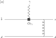
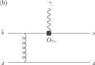
Figure 3: Feynman diagrams of electromagnetic penguin operator ${O_{7\gamma}}$. A photon is emitted through the ${O_{7\gamma}}$ operator, and one hard gluon exchange is needed to form hadrons.

$$M_{7\gamma}^{S(a)} = -M_{7\gamma}^{P(a)}$$ (14)

$$= -2\hskip 2.84526ptF^{(0)}\xi_{t}\int^{1}_{0}dx_{1}dx_{2}\int b_{1}db_{1}b_{2}db_{2}\phi_{B}(x_{1},b_{1})S_{t}(x_{1})\alpha_{s}(t_{7}^{a})e^{\left[-S_{B}(t_{7}^{a})-S_{K^{*}}(t_{7}^{a})\right]}C_{7}(t_{7}^{a})$$

$$\times H_{7}^{(a)}\left(A_{7}b_{2},B_{7}b_{1},B_{7}b_{2}\right)r_{K^{\ast}}\left[\phi_{K^{\ast}}^{v}(x_{2})+\phi_{K^{\ast}}^{a}(x_{2})\right]\hskip 14.22636pt\left(t_{7}^{a}=\mbox{max}(A_{7},B_{7},1/b_{1},1/b_{2})\right)$$

$$M_{7\gamma}^{S(b)} = -M_{7\gamma}^{P(b)}$$ (15)

$$= -2\hskip 2.84526ptF^{(0)}\xi_{t}\int^{1}_{0}dx_{1}dx_{2}\int b_{1}db_{1}\hskip 2.84526ptb_{2}db_{2}\phi_{B}(x_{1},b_{1})~{}S_{t}(x_{2})\hskip 2.84526pt\alpha_{s}(t_{7}^{b})e^{\left[-S_{B}(t_{7}^{b})-S_{K^{*}}(t_{7}^{b})\right]}C_{7}(t_{7}^{b})$$

$$\times H_{7}^{(b)}(A_{7}b_{1},C_{7}b_{1},C_{7}b_{2})\Big{[}(1-2x_{2})r_{K^{*}}(\phi_{K^{\ast}}^{v}(x_{2})+\phi_{K^{\ast}}^{a}(x_{2}))+(1+x_{2})\phi_{K^{\ast}}^{T}(x_{2})\Big{]}$$

$$\hskip 71.13188pt\left(t_{7}^{b}=\mbox{max}(A_{7},C_{7},1/b_{1},1/b_{2})\right)$$

$$H_{7}^{(a)}\left(A_{7}b_{2},B_{7}b_{1},B_{7}b_{2}\right)\equiv K_{0}(A_{7}b_{2})\Big{[}\theta(b_{1}-b_{2})K_{0}\left(B_{7}b_{1}\right)I_{0}\left(B_{7}b_{2}\right)+\theta(b_{2}-b_{1})K_{0}\left(B_{7}b_{2}\right)I_{0}\left(B_{7}b_{1}\right)\Big{]}$$ (16)

$$H_{7}^{(b)}(A_{7}b_{1},C_{7}b_{1},C_{7}b_{2})=H_{7}^{(a)}(A_{7}b_{1},C_{7}b_{1},C_{7}b_{2})$$ (17)

$$A_{7}^{2}=x_{1}x_{2}M_{B}^{2},\hskip 14.22636ptB_{7}^{2}=x_{1}{M_{B}}^{2}\hskip 14.22636ptC_{7}^{2}=x_{2}M_{B}^{2}\hskip 14.22636pt$$ (18)

Here ${K_{0}}$, ${I_{0}}$ are modified Bessel functions which come from propagator integrations. The meson wave functions are not calculable because of its nonperturbative feature. But they should be universal since they absorb long-distance dynamics, so we can use the meson wave functions determined by some approaches. We use in this paper a model ${B}$ meson wave function which is shown to give adequate form factors for ${B\to K\pi}$ decays Bauer:fx ; Keum:2000ph , and ${K^{*}}$ meson determined by light-cone QCD sum rule Ball:1998ff ; Ball:2003sc . Their explicit formulas are shown in Appendix B.

IV.2 ${O_{8g}}$ contribution

Similarly, we can calculate the ${O_{8g}}$ contributions as follows. In these cases, a hard gluon is emitted through the ${O_{8g}}$ operator and glued to the spectator quark line (Fig.4). In the following formulas, ${Q_{q}}$ express the electric charge of the external quark: ${Q_{u}=2/3}$ and ${Q_{d}=Q_{s}=Q_{b}=-1/3}$.

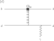
Figure 4: Feynman diagrams of chromomagnetic penguin operator ${O_{8g}}$. A hard gluon is emitted through the ${O_{8g}}$ operator and glued to the spectator quark line. Then photon is emitted by bremsstrahlung of external quark lines.

$$M_{8}^{S(a)} = -M_{8}^{P(a)}$$ (19)

$$= -F^{(0)}\xi_{t}Q_{b}\int^{1}_{0}dx_{1}dx_{2}\int b_{1}db_{1}\hskip 2.84526ptb_{2}db_{2}\hskip 2.84526pt\phi_{B}(x_{1},b_{1})S_{t}(x_{1})\alpha_{s}(t_{8}^{a})e^{\left[-S_{B}(t_{8}^{a})-S_{K^{*}}(t_{8}^{a})\right]}C_{8}(t_{8}^{a})H_{8}^{(a)}(A_{8}b_{2},B_{8}b_{1},B_{8}b_{2})$$

$$\times [x_{1}\phi_{K^{*}}^{T}(x_{2})+r_{K^{*}}x_{2}(\phi_{K^{*}}^{v}(x_{2})+\phi_{K^{*}}^{a}(x_{2}))]\hskip 14.22636pt\left(t_{8}^{a}=\mbox{max}(A_{8},B_{8},1/b_{1},1/b_{2})\right)$$

$$M_{8}^{S(b)} = -M_{8}^{P(b)}$$ (20)

$$= -F^{(0)}\xi_{t}Q_{s}\int^{1}_{0}dx_{1}dx_{2}\int b_{1}db_{1}\hskip 2.84526ptb_{2}db_{2}\hskip 2.84526pt\phi_{B}(x_{1},b_{1})S_{t}(x_{2})\alpha_{s}(t_{8}^{b})\hskip 2.84526pte^{\left[-S_{B}(t_{8}^{b})-S_{K^{*}}(t_{8}^{b})\right]}C_{8}(t_{8}^{b})H_{8}^{(b)}(A_{8}b_{1},C_{8}b_{1},C_{8}b_{2})$$

$$\times [-3x_{2}r_{K^{*}}(\phi_{K^{*}}^{v}(x_{2})+\phi_{K^{*}}^{a}(x_{2}))+(2x_{2}-x_{1})\phi_{K^{*}}^{T}(x_{2})]\hskip 14.22636pt\left(t_{8}^{b}=\mbox{max}(A_{8},C_{8},1/b_{1},1/b_{2})\right)$$

$$M_{8}^{S(c)} = -M_{8}^{P(c)}$$ (21)

$$= -F^{(0)}\xi_{t}Q_{q}\int^{1}_{0}dx_{1}dx_{2}\int b_{1}db_{1}\hskip 2.84526ptb_{2}db_{2}\hskip 2.84526pt\phi_{B}(x_{1},b_{1})S_{t}(x_{1})\alpha_{s}(t_{8}^{c})\hskip 2.84526pte^{\left[-S_{B}(t_{8}^{c})-S_{K^{*}}(t_{8}^{c})\right]}C_{8}(t_{8}^{c})H_{8}^{(c)}(\sqrt{|A_{8}^{\prime 2}|}b_{2},D_{8}b_{1},D_{8}b_{2})$$

$$\times[-x_{1}\phi_{K^{*}}^{T}(x_{2})+x_{2}r_{K^{*}}(\phi_{K^{*}}^{v}(x_{2})+\phi_{K^{\ast}}^{a}(x_{2}))]\hskip 14.22636pt\left(t_{8}^{c}=\mbox{max}(\sqrt{\mid A_{8}^{\prime 2}\mid},D_{8},1/b_{1},1/b_{2})\right)$$

$$M_{8}^{S(d)} = -F^{(0)}\xi_{t}Q_{q}\int^{1}_{0}dx_{1}dx_{2}\int b_{1}db_{1}\hskip 2.84526ptb_{2}db_{2}\hskip 2.84526pt\phi_{B}(x_{1},b_{1})S_{t}(x_{2})\alpha_{s}(t_{8}^{d})\hskip 2.84526pte^{\left[-S_{B}(t_{8}^{d})-S_{K^{\ast}}(t_{8}^{d})\right]}C_{8}(t_{8}^{d})H_{8}^{(d)}(\sqrt{|A_{8}^{\prime 2}|}b_{1},E_{8}b_{1},E_{8}b_{2})$$ (22)

$$\times [~{}6x_{2}r_{K^{\ast}}\phi_{K^{\ast}}^{v}(x_{2})+(2+x_{2}-x_{1})\phi_{K^{\ast}}^{T}(x_{2})]$$

$$M_{8}^{P(d)} = F^{(0)}\xi_{t}Q_{q}\int^{1}_{0}dx_{1}dx_{2}\int b_{1}db_{1}\hskip 2.84526ptb_{2}db_{2}\hskip 2.84526pt\phi_{B}(x_{1},b_{1})S_{t}(x_{2})\alpha_{s}(t_{8}^{d})\hskip 2.84526pte^{\left[-S_{B}(t_{8}^{d})-S_{K^{\ast}}(t_{8}^{d})\right]}C_{8}(t_{8}^{d})H_{8}^{(d)}(\sqrt{|A_{8}^{\prime 2}|}b_{1},E_{8}b_{1},E_{8}b_{2})$$ (23)

$$\times [~{}(2+x_{2}-x_{1})\phi_{K^{\ast}}^{T}(x_{2})+6x_{2}r_{K^{\ast}}\phi_{K^{\ast}}^{a}(x_{2})]\hskip 14.22636pt\left(t_{8}^{d}=\mbox{max}(\sqrt{|A_{8}^{\prime 2}|},E_{8},1/b_{1},1/b_{2})\right)$$

$$H_{8}^{(a)}(A_{8}b_{2},B_{8}b_{1},B_{8}b_{2})\equiv K_{0}(A_{8}b_{2})\Big{[}\theta(b_{1}-b_{2})K_{0}(B_{8}b_{1})I_{0}(B_{8}b_{2})+(b_{1}\leftrightarrow b_{2})\Big{]}$$ (24)

$$H_{8}^{(b)}(A_{8}b_{1},C_{8}b_{1},C_{8}b_{2})\equiv\frac{i\pi}{2}K_{0}(A_{8}b_{1})\Big{[}\theta(b_{1}-b_{2})H_{0}^{(1)}(C_{8}b_{1})J_{0}(C_{8}b_{2})+(b_{1}\leftrightarrow b_{2})\Big{]}$$ (25)

$$H_{8}^{(c)}(\sqrt{|A_{8}^{\prime 2}|}b_{2},D_{8}b_{1},D_{8}b_{2})\equiv\theta(A_{8}^{\prime 2})\hskip 2.84526ptK_{0}(\sqrt{|A_{8}^{\prime 2}|}b_{2})\Big{[}\theta(b_{1}-b_{2})K_{0}(D_{8}b_{1})I_{0}(D_{8}b_{2})+(b_{1}\leftrightarrow b_{2})\Big{]}$$

$$\hskip 113.81102pt+\theta(-A_{8}^{\prime 2})\hskip 2.84526pti\frac{\pi}{2}H_{0}^{(1)}(\sqrt{|A_{8}^{\prime 2}|}b_{2})\Big{[}\theta(b_{1}-b_{2})K_{0}(D_{8}b_{1})I_{0}(D_{8}b_{2})+(b_{1}\leftrightarrow b_{2})\Big{]}$$ (26)

$$H_{8}^{(d)}(\sqrt{|A_{8}^{\prime 2}|}b_{1},E_{8}b_{1},E_{8}b_{2})\equiv\theta(A_{8}^{\prime 2})\hskip 2.84526pti\frac{\pi}{2}K_{0}(\sqrt{|A_{8}^{\prime 2}|}b_{1})\left[\theta(b_{1}-b_{2})H_{0}^{(1)}(E_{8}b_{1})J_{0}(E_{8}b_{2})+(b_{1}\leftrightarrow b_{2})\right]$$

$$\hskip 113.81102pt-\theta(-A_{8}^{\prime 2})\hskip 2.84526pt\left(\frac{\pi}{2}\right)^{2}H_{0}^{(1)}(\sqrt{|A_{8}^{\prime 2}}|b_{1})\left[\theta(b_{1}-b_{2})H_{0}^{(1)}(E_{8}b_{1})J_{0}(E_{8}b_{2})+(b_{1}\leftrightarrow b_{2})\right]$$ (27)

$$A_{8}^{2}=x_{1}x_{2}M_{B}^{2},\hskip 8.53581ptB_{8}^{2}=M_{B}^{2}(1+x_{1}),\hskip 8.53581ptC_{8}^{2}=M_{B}^{2}(1-x_{2}),\hskip 8.53581ptA_{8}^{\prime 2}=(x_{1}-x_{2})M_{B}^{2},\hskip 8.53581ptD_{8}^{2}=x_{1}{M_{B}}^{2},\hskip 8.53581ptE_{8}^{2}=x_{2}{M_{B}}^{2}$$ (28)

IV.3 Loop contributions

IV.3.1 Quark line photon emission

Next we want to mention about charm and up quark penguin contributions (Fig.5). The subtitle like “Quark line photon emission” means that a photon is emitted through the external quark lines.

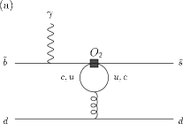
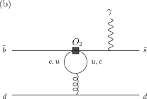
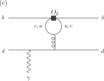
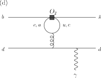
Figure 5: Feynman diagrams of “Quark line photon emission”. The charm or up loop go to gluon and attach to the spectator quark line. A photon is emitted through the external quark lines.

We define the ${c}$ and ${u}$ loop function in order that the ${b\to sg}$ vertex can be expressed as ${\bar{s}\gamma^{\mu}(1-\gamma^{5})I_{\mu\nu}b}$. It has the gauge invariant form Bander:px and the explicit formula is as follows,

$$I_{\mu\nu}^{a} = \frac{gT^{a}}{2\pi^{2}}(k^{2}g_{\mu\nu}-k_{\mu}k_{\nu})\int^{1}_{0}dxx(1-x)\left[1+\log\left[\frac{m_{i}^{2}-x(1-x)k^{2}}{t^{2}}\right]\right]$$ (29)

$$= -\frac{gT^{a}}{8\pi^{2}}(k^{2}g_{\mu\nu}-k_{\mu}k_{\nu})\left[G(m_{i}^{2},k^{2},t)-\frac{2}{3}\right],$$

where ${k}$ is the gluon momentum and ${m_{i}}$ is the loop internal quark mass.

$$G(m_{i}^{2},k^{2},t) = \theta(-k^{2})\frac{2}{3}\Big{[}\frac{5}{3}+\frac{4m_{i}^{2}}{k^{2}}-\ln{\frac{m_{i}^{2}}{t^{2}}}+\left(1+\frac{2m_{i}^{2}}{k^{2}}\right)\sqrt{1-\frac{4m_{i}^{2}}{k^{2}}}\ln{\frac{\sqrt{1-4m_{i}^{2}/k^{2}}-1}{\sqrt{1-4m_{i}^{2}/k^{2}}+1}}\Big{]}$$

$$+\theta(k^{2})\theta(4m_{i}^{2}-k^{2})\frac{2}{3}\Big{[}\frac{5}{3}+\frac{4m_{i}^{2}}{k^{2}}-\ln{\frac{m_{i}^{2}}{t^{2}}}-2\left(1+\frac{2m_{i}^{2}}{k^{2}}\right)\sqrt{\frac{4m_{i}^{2}}{k^{2}}-1}\arctan{\left(\frac{1}{\sqrt{4m_{i}^{2}/k^{2}-1}}\right)}\Big{]}$$

$$+\theta(k^{2}-4m_{i}^{2})\frac{2}{3}\Big{[}\frac{5}{3}+\frac{4m_{i}^{2}}{k^{2}}-\ln{\frac{m_{i}^{2}}{t^{2}}}+\left(1+\frac{2m_{i}^{2}}{k^{2}}\right)\sqrt{1-\frac{4m_{i}^{2}}{k^{2}}}\left[\ln{\frac{1-\sqrt{1-4m_{i}^{2}/k^{2}}}{1+\sqrt{1-4m_{i}^{2}/k^{2}}}}+i\pi\right]\Big{]}$$

The loop function ${G}$ has the dependence of gluon momentum square of ${k^{2}}$. But there is no singularity when we take the limit of ${k\rightarrow 0}$, so we can neglect ${k_{T}}$ components of ${k^{2}}$ in the loop function ${G}$.

Then the “Quark line photon emission” contributions can be expressed as follows.

$$M_{1i}^{S(a)} = M_{1i}^{P(a)}$$ (31)

$$= \frac{Q_{b}}{2}F^{(0)}\xi_{i}\int^{1}_{0}dx_{1}dx_{2}\int b_{1}db_{1}b_{2}db_{2}\phi_{B}(x_{1},b_{1})C_{2}(t_{2}^{a})\alpha_{s}(t_{2}^{a})S_{t}(x_{1})e^{\left[-S_{B}(t_{2}^{a})-S_{K^{*}}(t_{2}^{a})\right]}H_{2}^{(a)}(A_{2}b_{2},B_{2}b_{1},B_{2}b_{2})$$

$$\times\Big{[}G(m_{i}^{2},-A_{2}^{2},t_{2}^{a})-\frac{2}{3}\Big{]}x_{1}x_{2}r_{K^{*}}(\phi_{K^{*}}^{v}(x_{2})-\phi_{K^{*}}^{a}(x_{2}))\hskip 14.22636pt\left(t_{2}^{a}=\mbox{max}(A_{2},B_{2},\hskip 2.84526pt1/b_{1},1/b_{2})\right)$$

$$M_{1i}^{S(b)} = -M_{1i}^{P(b)}$$ (32)

$$= -\frac{Q_{s}}{2}F^{(0)}\hskip 2.84526pt\xi_{i}\int^{1}_{0}dx_{1}dx_{2}\int b_{1}db_{1}b_{2}db_{2}\phi_{B}(x_{1},b_{1})C_{2}(t_{2}^{b})\alpha_{s}(t_{2}^{b})S_{t}(x_{2})e^{\left[-S_{B}(t_{2}^{b})-S_{K^{*}}(t_{2}^{b})\right]}H_{2}^{(b)}(A_{2}b_{1},C_{2}b_{1},C_{2}b_{2}^{b})$$

$$\times\Big{[}G(m_{i}^{2},-A_{2}^{2},t_{2}^{b})-\frac{2}{3}\Big{]}\Big{[}x_{2}^{2}r_{K^{*}}(\phi_{K^{*}}^{v}(x_{2})+\phi_{K^{*}}^{a}(x_{2}))+3x_{1}x_{2}\phi_{K^{*}}^{T}(x_{2})\Big{]}\hskip 14.22636pt\left(t_{2}^{b}=\mbox{max}(A_{2},C_{2},\hskip 2.84526pt1/b_{1},1/b_{2})\right)$$

$$M_{1i}^{S(c)} = -M_{1i}^{P(c)}$$ (33)

$$= \frac{Q_{q}}{2}F^{(0)}\hskip 2.84526pt\xi_{i}\int^{1}_{0}dx_{1}dx_{2}\int b_{1}db_{1}b_{2}db_{2}\phi_{B}(x_{1},b_{1})C_{2}(t_{2}^{c})\alpha_{s}(t_{2}^{c})S_{t}(x_{1})e^{\left[-S_{B}(t_{2}^{c})-S_{K^{*}}(t_{2}^{c})\right]}H_{2}^{(c)}(\sqrt{|A_{2}^{{}^{\prime}2}|}b_{2},D_{2}b_{1},D_{2}b_{2})$$

$$\times\Big{[}G(m_{i}^{2},-A_{2}^{{}^{\prime}2},t_{2}^{c})-\frac{2}{3}\Big{]}\Big{[}x_{2}r_{K^{*}}(\phi_{K^{*}}^{v}(x_{2})+\phi_{K^{*}}^{a}(x_{2}))-x_{1}\phi_{K^{*}}^{T}(x_{2})\Big{]}\hskip 14.22636pt\left(t_{2}^{c}=\mbox{max}(\sqrt{|A_{2}^{{}^{\prime}2}|},D_{2},\hskip 2.84526pt1/b_{1},1/b_{2})\right)$$

$$M_{1i}^{S(d)} = \frac{Q_{q}}{2}F^{(0)}\hskip 2.84526pt\xi_{i}\int^{1}_{0}dx_{1}dx_{2}\int b_{1}db_{1}b_{2}db_{2}\phi_{B}(x_{1},b_{1})C_{2}(t_{2}^{d})\alpha_{s}(t_{2}^{d})S_{t}(x_{2})e^{\left[-S_{B}(t_{2}^{d})-S_{K^{*}}(t_{2}^{d})\right]}H_{2}^{(d)}(\sqrt{|A_{2}^{{}^{\prime}2}|}b_{1},E_{2}b_{1},E_{2}b_{2})$$ (34)

$$\times\Big{[}G(m_{i}^{2},-A_{2}^{{}^{\prime}2},t_{2}^{d})-\frac{2}{3}\Big{]}\Big{[}x_{2}r_{K^{*}}[3(1+x_{2})\phi_{K^{*}}^{v}(x_{2})-(1-x_{2})\phi_{K^{*}}^{a}(x_{2})]+3(x_{2}-x_{1})\phi_{K^{*}}^{T}(x_{2})\Big{]}$$

$$M_{1i}^{P(d)} = -\frac{Q_{q}}{2}F^{(0)}\hskip 2.84526pt\xi_{i}\int^{1}_{0}dx_{1}dx_{2}\int b_{1}db_{1}b_{2}db_{2}\phi_{B}(x_{1},b_{1})C_{2}(t_{2}^{d})\alpha_{s}(t_{2}^{d})S_{t}(x_{2})e^{\left[-S_{B}(t_{2}^{d})-S_{K^{*}}(t_{2}^{d})\right]}H_{2}^{(d)}(\sqrt{|A_{2}^{{}^{\prime}2}|}b_{1},E_{2}b_{1},E_{2}b_{2})$$ (35)

$$\times\Big{[}G(m_{i}^{2},-A_{2}^{{}^{\prime}2},t_{2}^{d})-\frac{2}{3}\Big{]}\Big{[}x_{2}r_{K^{*}}[-(1-x_{2})\phi_{K^{*}}^{v}(x_{2})+3(1+x_{2})\phi_{K^{*}}^{a}(x_{2})]+3(x_{2}-x_{1})\phi_{K^{*}}^{T}(x_{2})\Big{]}$$

$$\hskip 113.81102pt\left(t_{2}^{d}=\mbox{max}(\sqrt{|A_{2}^{{}^{\prime}2}|},E_{2},\hskip 2.84526pt1/b_{1},1/b_{2})\right)$$

$$H_{2}^{(a)}(A_{2}b_{2},B_{2}b_{1},B_{2}b_{2}) = H_{8}^{(a)}(A_{8}b_{2},B_{8}b_{1},B_{8}b_{2})$$

$$H_{2}^{(b)}(A_{2}b_{1},C_{2}b_{1},C_{2}b_{2}) = H_{8}^{(b)}(A_{8}b_{1},C_{8}b_{1},C_{8}b_{2})$$

$$H_{2}^{(c)}(\sqrt{|A_{2}^{{}^{\prime}2}|}b_{2},D_{2}b_{1},D_{2}b_{2}) = H_{8}^{(c)}(\sqrt{|A_{8}^{{}^{\prime}2}|}b_{2},D_{8}b_{1},D_{8}b_{2})$$ (36)

$$H_{2}^{(d)}(\sqrt{|A_{2}^{{}^{\prime}2}|}b_{1},E_{2}b_{1},E_{2}b_{2}) = H_{8}^{(d)}(\sqrt{|A_{8}^{{}^{\prime}2}|}b_{1},E_{8}b_{1},E_{8}b_{2})$$

$$A_{2}^{2}=x_{1}x_{2}M_{B}^{2},\hskip 8.53581ptB_{2}^{2}=(1+x_{1})M_{B}^{2},\hskip 8.53581ptC_{2}^{2}=(1-x_{2})M_{B}^{2},\hskip 8.53581ptA_{2}^{{}^{\prime}2}=(x_{1}-x_{2})M_{B}^{2},\hskip 8.53581ptD_{2}^{2}=x_{1}M_{B}^{2},\hskip 8.53581ptE_{2}^{2}=x_{2}M_{B}^{2}$$ (37)

IV.3.2 Loop line photon emission

Next we consider the “Loop line photon emission”: a photon is emitted through the ${c}$ or ${u}$ quark loop line.

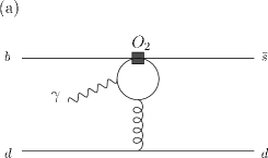
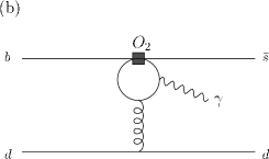
Figure 6: The Feynman diagrams of “Loop line photon emission”. The charm or up loop go to gluon and attach to the spectator quark line. A photon is emitted by bremsstrahlung of loop quark line.

We sum up Fig.6(a) and 6(b), the ${b\to sg\gamma}$ decay amplitude is expressed as

$$A(b\to sg\gamma)=\epsilon_{\gamma}^{\mu}(q)\epsilon_{a}^{\nu}(k)\hskip 2.84526pt\bar{s}(p^{\prime})I_{\mu\nu}^{a}b(p),$$ (38)

where vertex function ${I_{\mu\nu}}$ is defined as follows Liu:1990yb ; Simma:nr ; Li:1998tk ,

$$I_{\mu\nu}^{a} = F_{1}^{a}\Big{[}(k\cdot q)\epsilon_{\mu\nu\rho\sigma}\hskip 2.84526pt(q^{\rho}-k^{\rho})\gamma^{\sigma}+q_{\nu}\epsilon_{\mu\rho\sigma\delta}\hskip 2.84526ptq^{\rho}k^{\sigma}\gamma^{\delta}-k_{\mu}\epsilon_{\nu\rho\sigma\delta}\hskip 2.84526ptq^{\rho}k^{\sigma}\gamma^{\delta}\Big{]}L$$ (39)

$$+F_{2}^{a}\Big{[}k_{\nu}\epsilon_{\mu\rho\sigma\delta}\hskip 2.84526ptq^{\rho}k^{\sigma}\gamma^{\delta}+k^{2}\hskip 2.84526pt\epsilon_{\mu\nu\rho\sigma}\hskip 2.84526ptq^{\rho}\gamma^{\sigma}\Big{]}L,$$

$$F_{1}^{a} = -\frac{i2\sqrt{2}}{3\pi^{2}}egT^{a}G_{F}\int^{1}_{0}dx\int^{1-x}_{0}dy\frac{xy}{m_{i}^{2}-2xy(k\cdot q)-k^{2}x(1-x)},$$ (40)

$$F_{2}^{a} = -\frac{i2\sqrt{2}}{3\pi^{2}}egT^{a}G_{F}\int^{1}_{0}dx\int^{1-x}_{0}dy\frac{x(1-x)}{m_{i}^{2}-2xy(k\cdot q)-k^{2}x(1-x)},$$ (41)

where ${L=(1-\gamma^{5})/2}$, ${k}$ is the gluon momentum and ${q}$ is the photon one. Then the amplitudes can be expressed as follows:

$$M_{2i}^{S} = -\frac{4}{3}F^{(0)}\xi_{i}\int^{1}_{0}dx\int^{1-x}_{0}dy\int^{1}_{0}dx_{1}dx_{2}\int b_{1}db_{1}\phi_{B}(x_{1},b_{1})C_{2}(t_{2})\alpha_{s}(t_{2})e^{\left[-S_{B}(t_{2})-S_{K^{*}}(t_{2})\right]}H_{2}(b_{1}A,b_{1}\sqrt{|B^{2}|})$$

$$\times\frac{1}{xyx_{2}M_{B}^{2}-m_{i}^{2}}\Big{[}xyx_{2}\Big{[}(1-2x_{2})r_{K^{*}}\phi_{K^{*}}^{v}(x_{2})-(1+2x_{1})\phi_{K^{*}}^{T}(x_{2})+r_{K^{*}}\phi_{K^{*}}^{a}(x_{2})\Big{]}$$

$$\hskip 113.81102pt+x(1-x)\Big{[}x_{2}^{2}r_{K^{*}}(\phi_{K^{*}}^{v}(x_{2})+\phi_{K^{*}}^{a}(x_{2}))+3x_{1}x_{2}\phi_{K^{*}}^{T}(x_{2})\Big{]}\Big{]}$$

$$M_{2i}^{P} = \frac{4}{3}F^{(0)}\xi_{i}\int^{1}_{0}dx\int^{1-x}_{0}dy\int^{1}_{0}dx_{1}dx_{2}\int b_{1}db_{1}\phi_{B}(x_{1},b_{1})C_{2}(t_{2})\alpha_{s}(t_{2})e^{\left[-S_{B}(t_{2})-S_{K^{*}}(t_{2})\right]}H_{2}(b_{1}A,b_{1}\sqrt{|B^{2}|})$$ (43)

$$\times\frac{1}{xyx_{2}M_{B}^{2}-m_{i}^{2}}\Big{[}xyx_{2}\Big{[}r_{K^{*}}\phi_{K^{*}}^{v}(x_{2})-(1+2x_{1})\phi_{K^{*}}^{T}(x_{2})+(1-2x_{2})r_{K^{*}}\phi_{K^{*}}^{a}(x_{2})\Big{]}$$

$$\hskip 113.81102pt+x(1-x)[x_{2}^{2}r_{K^{*}}(\phi_{K^{*}}^{v}(x_{2})+\phi_{K^{*}}^{a}(x_{2}))+3x_{1}x_{2}\phi_{K^{*}}^{T}(x_{2})]\Big{]}$$

$$\hskip 85.35826pt\left(t_{2}=\mbox{max}(A,\sqrt{|B^{2}|},\hskip 2.84526pt1/b_{1})\right)$$

$$H_{2}(b_{1}A,b_{1}\sqrt{|B^{2}|}) \equiv K_{0}(b_{1}A)-K_{0}(b_{1}\sqrt{|B^{2}|})\hskip 14.22636pt(B^{2}\geq 0)$$ (44)

$$\equiv K_{0}(b_{1}A)-i\frac{\pi}{2}H_{0}(b_{1}\sqrt{|B^{2}|})\hskip 8.53581pt(B^{2}<0)$$

$$A^{2}=x_{1}x_{2}M_{B}^{2},\hskip 14.22636ptB^{2}=x_{1}x_{2}M_{B}^{2}-\frac{y}{1-x}x_{2}M_{B}^{2}+\frac{m_{i}^{2}}{x(1-x)}$$ (45)

In general, it is hard to estimate the ${u}$ loop contributions accurately because of the nonperturbative hadronic uncertainties. For ${k^{2}<1}$GeV, nonperturbative correction to the ${u}$ quark loop shown in Fig.7 is large and in fact ${u\bar{u}}$ pair may be better represented by resonances. On the other hand if ${k^{2}}$ is large, the perturbative computation is expected to be reliable.

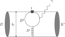
Figure 7: The energy scale of the loop contribution is ${t=\mbox{max}(A,\sqrt{|B|^{2}},1/b_{1})}$, where ${A^{2}}$ is gluon momentum , ${B^{2}}$ is the loop momentum, and ${b_{1}}$ is the transverse interval between the quark and antiquark pair in the ${B}$ meson.

In the pQCD approach, the factorization energy scale ${t}$ is determined at each point of the integration, i.e. for each point ${(x_{1},x_{2},b_{1},b_{2})}$. Then these variables are integrated over the entire physical region. So for each point ${(x_{1},x_{2},b_{1},b_{2})}$, ${\alpha_{s}(t)}$ can be determined. Thus we can observe the contribution to the amplitude as a function of ${\alpha_{s}(t)}$. Figures 9 and 9 show the distribution of ${\alpha_{s}(t)}$ for a diagram with the ${c}$ quark loop, and ${u}$ quark loop, respectively. We can see that the major part of the ${c}$ loop contribution comes from a perturbative region, on the other hand ${u}$ loop contribution includes also a nonperturbative region. Since ${M_{2u}^{S}}$ and ${M_{2u}^{P}}$ gets considerable contributions from the nonperturbative region, we introduce 100% theoretical error for these amplitudes.

Figure 8: The horizontal line is ${\alpha_{s}(t)/\pi}$ and the vertical axis is the contribution from the each energy region in ${\alpha_{s}}$ to the total decay amplitude. The left figure is the real part and right one is imaginary part of the ${c}$ loop contribution. These figures show that we can compute the ${c}$ quark loop contribution perturbatively.

Figure 9: The horizontal line is ${\alpha_{s}(t)/\pi}$ and the vertical axis is the distribution from the each energy region in ${\alpha_{s}}$ to the total decay amplitude. The left figure is the real part and right one is imaginary part of the ${u}$ loop contribution. These figures show that nonperturbative contributions are important, so we cannot accurately compute the ${u}$ quark loop contribution and have to take into account the hadronic uncertainty.

IV.4 Annihilation contributions

IV.4.1 Tree annihilation

We now discuss the annihilation contributions caused by ${O_{1}}$ and ${O_{2}}$ operators. The diagrams are shown in Fig.10.

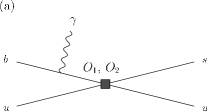
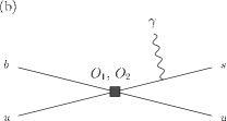
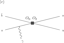
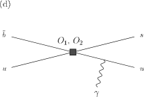
Figure 10: Annihilation diagrams caused by ${O_{1}}$, ${O_{2}}$ operators. In these cases, no hard gluons are needed because they are four Fermi interactions and do not include spectator quarks which should be line up to form hadrons.

The operators ${O_{1}}$, ${O_{2}}$ can be rewritten as

$$O_{1} = (\bar{s}_{i}u_{j})_{V-A}(\bar{u}_{j}b_{i})_{V-A}=(\bar{s}_{i}b_{i})_{V-A}(\bar{u}_{j}u_{j})_{V-A},\hskip 5.69054pt$$ (46)

$$O_{2} = (\bar{s}_{i}u_{i})_{V-A}(\bar{u}_{j}b_{j})_{V-A}=(\bar{s}_{i}b_{j})_{V-A}(\bar{u}_{j}u_{i})_{V-A}.$$ (47)

These annihilation contributions are tree processes: no hard gluons are needed because they are four Fermi interaction processes and do not include spectator quarks which should be line up to form hadrons. However, these contributions are small because it has ${(V-A)\otimes(V-A)}$ vertex: gets chiral suppression, and its’ CKM factor is ${V_{ub}^{*}V_{us}}$, ${O(\lambda^{2})}$ suppression compared to ${V_{tb}^{*}V_{ts}}$ and ${V_{cb}^{*}V_{cs}}$. Defining ${a_{2}(t)=C_{2}(t)+C_{1}(t)/3}$, the each decay amplitudes are as follows:

$$M_{2}^{S(a)} = M_{2}^{P(a)}$$ (48)

$$= -F^{(0)}\xi_{u}\frac{3\sqrt{6}Q_{b}f_{K^{*}}\pi}{4M_{B}^{2}}r_{K^{*}}\int^{1}_{0}dx_{1}\int b_{1}db_{1}$$

$$a_{2}(t_{a}^{a})S_{t}(x_{1})\hskip 2.84526pte^{\left[-S_{B}(t_{a}^{a})\right]}\phi_{B}(x_{1},b_{1})K_{0}(b_{1}A_{a})$$

$$\hskip 14.22636pt\left(t_{a}^{a}=\mbox{max}(A_{a},1/b_{1})\right)$$

$$M_{2}^{S(b)} = -F^{(0)}\xi_{u}\frac{3\sqrt{6}Q_{s}f_{B}\pi}{4M_{B}^{2}}r_{K^{*}}\int^{1}_{0}dx_{2}\int b_{2}db_{2}$$ (49)

$$a_{2}(t_{a}^{b})S_{t}(x_{2})\hskip 2.84526pte^{\left[-S_{K^{*}}(t_{a}^{b})\right]}i\frac{\pi}{2}H_{0}^{(1)}(b_{2}B_{a})$$

$$\times \Big{[}(2-x_{2})\phi_{K^{*}}^{v}(x_{2})+x_{2}\phi_{K^{*}}^{a}(x_{2})\Big{]}$$

$$M_{2}^{P(b)} = F^{(0)}\xi_{u}\frac{3\sqrt{6}Q_{s}f_{B}\pi}{4M_{B}^{2}}r_{K^{*}}\int^{1}_{0}dx_{2}\int b_{2}db_{2}$$ (50)

$$a_{2}(t_{a}^{b})S_{t}(x_{2})\hskip 2.84526pte^{\left[-S_{K^{*}}(t_{a}^{b})\right]}i\frac{\pi}{2}H_{0}^{(1)}(b_{2}B_{a})$$

$$\times \left[x_{2}\phi_{K^{*}}^{v}(x_{2})+(2-x_{2})\phi_{K^{*}}^{a}(x_{2})\right]$$

$$\hskip 14.22636pt\left(t_{a}^{b}=\mbox{max}(B_{a},1/b_{2})\right)$$

$$M_{2}^{S(c)} = -M_{2}^{P(c)}$$ (51)

$$= F^{(0)}\xi_{u}\frac{3\sqrt{6}Q_{u}f_{K^{*}}\pi}{4M_{B}^{2}}r_{K^{*}}\int^{1}_{0}dx_{1}\int b_{1}db_{1}$$

$$a_{2}(t_{a}^{c})S_{t}(x_{1})e^{\left[-S_{B}(t_{a}^{c})\right]}\phi_{B}(x_{1},b_{1})K_{0}(b_{1}C_{a})$$

$$\hskip 14.22636pt\left(t_{a}^{c}=\mbox{max}(C_{a},1/b_{1})\right)$$

$$M_{2}^{S(d)} = F^{(0)}\xi_{u}\frac{3\sqrt{6}Q_{u}f_{B}\pi}{4M_{B}^{2}}r_{K^{*}}\int^{1}_{0}dx_{2}\int b_{2}db_{2}$$ (52)

$$a_{2}(t_{a}^{d})S_{t}(x_{2})\hskip 2.84526pte^{\left[-S_{K^{*}}(t_{a}^{d})\right]}i\frac{\pi}{2}H_{0}^{(1)}(b_{2}D_{a})$$

$$\times \left[(1+x_{2})\phi_{K^{*}}^{v}(x_{2})-(1-x_{2})\phi_{K^{*}}^{a}(x_{2})\right]$$

$$M_{2}^{P(d)} = F^{(0)}\xi_{u}\frac{3\sqrt{6}Q_{u}f_{B}\pi}{4M_{B}^{2}}r_{K^{*}}\int^{1}_{0}dx_{2}\int b_{2}db_{2}$$ (53)

$$a_{2}(t_{a}^{d})S_{t}(x_{2})\hskip 2.84526pte^{\left[-S_{K^{*}}(t_{a}^{d})\right]}i\frac{\pi}{2}H_{0}^{(1)}(b_{2}D_{a})$$

$$\times \left[(1-x_{2})\phi_{K^{*}}^{v}(x_{2})-(1+x_{2})\phi_{K^{*}}^{a}(x_{2})\right]$$

$$\hskip 14.22636pt\left(t_{a}^{d}=\mbox{max}(D_{a},1/b_{2})\right)$$

$$A_{a}^{2}=(1+x_{1})M_{B}^{2},\hskip 28.45274ptB_{a}^{2}=(1-x_{2})M_{B}^{2},$$

$$C_{a}^{2}=x_{1}M_{B}^{2},\hskip 28.45274ptD_{a}^{2}=x_{2}M_{B}^{2}$$ (54)

IV.4.2 QCD Penguin

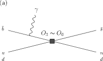
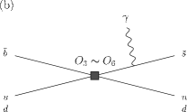
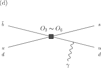
Figure 11: Annihilation diagrams caused by ${O_{3}\sim O_{6}}$ operators. QCD penguin annihilations include ${\alpha_{s}}$ in Wilson coefficient, so they are the same order of all contributions except for ${O_{1}}$, ${O_{2}}$ annihilations.

Next we mention the QCD penguin annihilation caused by ${O_{3}\sim O_{6}}$ operators like in Fig.11. Here we define ${a_{4}(t)=C_{4}(t)+C_{3}(t)/3,\hskip 5.69054pta_{6}(t)=C_{6}(t)+C_{5}(t)/3}$. ${O_{3}}$, ${O_{4}}$ have the same expression of ${O_{1}}$, ${O_{2}}$ annihilation contributions. ${O_{5}}$, ${O_{6}}$ have a ${(V-A)\otimes(V+A)}$ vertex so they have chiral enhancement compared to ${(V-A)\otimes(V-A)}$ vertex, and its’ CKM factor are ${V_{tb}^{*}V_{ts}}$, then its’ contributions are comparatively large and get main origins for isospin breaking effects.

$$M_{4}^{S(a)} = M_{4}^{P(a)}$$ (55)

$$= F^{(0)}\xi_{t}\frac{3\sqrt{6}Q_{b}f_{K^{*}}\pi}{4M_{B}^{2}}r_{K^{*}}\int^{1}_{0}dx_{1}\int b_{1}db_{1}$$

$$a_{4}(t_{a}^{a})S_{t}(x_{1})\hskip 2.84526pte^{\left[-S_{B}(t_{a}^{a})\right]}\phi_{B}(x_{1},b_{1})K_{0}(b_{1}A_{a})$$

$$\hskip 14.22636pt\left(t_{a}^{a}=\mbox{max}(A_{a},1/b_{1})\right)$$

$$M_{4}^{S(b)} = F^{(0)}\xi_{t}\frac{3\sqrt{6}Q_{s}f_{B}\pi}{4M_{B}^{2}}r_{K^{*}}\int^{1}_{0}dx_{2}\int b_{2}db_{2}$$ (56)

$$a_{4}(t_{a}^{b})S_{t}(x_{2})\hskip 2.84526pte^{\left[-S_{K^{*}}(t_{a}^{b})\right]}i\frac{\pi}{2}H_{0}^{(1)}(b_{2}B_{a})$$

$$\times \Big{[}(2-x_{2})\phi_{K^{*}}^{v}(x_{2})+x_{2}\phi_{K^{*}}^{a}(x_{2})\Big{]}$$

$$M_{4}^{P(b)} = -F^{(0)}\xi_{t}\frac{3\sqrt{6}Q_{s}f_{B}\pi}{4M_{B}^{2}}r_{K^{*}}\int^{1}_{0}dx_{2}\int b_{2}db_{2}$$ (57)

$$a_{4}(t_{a}^{b})S_{t}(x_{2})\hskip 2.84526pte^{\left[-S_{K^{*}}(t_{a}^{b})\right]}i\frac{\pi}{2}H_{0}^{(1)}(b_{2}B_{a})$$

$$\times \left[x_{2}\phi_{K^{*}}^{v}(x_{2})+(2-x_{2})\phi_{K^{*}}^{a}(x_{2})\right]$$

$$\hskip 14.22636pt\left(t_{a}^{b}=\mbox{max}(B_{a},1/b_{2})\right)$$

$$M_{4}^{S(c)} = -M_{4}^{P(c)}$$ (58)

$$= -F^{(0)}\xi_{t}\frac{3\sqrt{6}Q_{q}f_{K^{*}}\pi}{4M_{B}^{2}}r_{K^{*}}\int^{1}_{0}dx_{1}\int b_{1}db_{1}$$

$$a_{4}(t_{a}^{c})S_{t}(x_{1})e^{\left[-S_{B}(t_{a}^{c})\right]}\phi_{B}(x_{1},b_{1})K_{0}(b_{1}C_{a})$$

$$\hskip 14.22636pt\left(t_{a}^{c}=\mbox{max}(C_{a},1/b_{1})\right)$$

$$M_{4}^{S(d)} = -F^{(0)}\xi_{t}\frac{3\sqrt{6}Q_{q}f_{B}\pi}{4M_{B}^{2}}r_{K^{*}}\int^{1}_{0}dx_{2}\int b_{2}db_{2}$$ (59)

$$a_{4}(t_{a}^{d})S_{t}(x_{2})\hskip 2.84526pte^{\left[-S_{K^{*}}(t_{a}^{d})\right]}i\frac{\pi}{2}H_{0}^{(1)}(b_{2}D_{a})$$

$$\times \left[(1+x_{2})\phi_{K^{*}}^{v}(x_{2})-(1-x_{2})\phi_{K^{*}}^{a}(x_{2})\right]$$

$$M_{4}^{P(d)} = -F^{(0)}\xi_{t}\frac{3\sqrt{6}Q_{q}f_{B}\pi}{4M_{B}^{2}}r_{K^{*}}\int^{1}_{0}dx_{2}\int b_{2}db_{2}$$ (60)

$$a_{4}(t_{a}^{d})S_{t}(x_{2})\hskip 2.84526pte^{\left[-S_{K^{*}}(t_{a}^{d})\right]}i\frac{\pi}{2}H_{0}^{(1)}(b_{2}D_{a})$$

$$\times \left[(1-x_{2})\phi_{K^{*}}^{v}(x_{2})-(1+x_{2})\phi_{K^{*}}^{a}(x_{2})\right]$$

$$\hskip 14.22636pt\left(t_{a}^{d}=\mbox{max}(D_{a},1/b_{2})\right)$$

$$M_{6}^{S(b)} = -M_{6}^{P(b)}$$ (61)

$$= -F^{(0)}\xi_{t}\frac{3\sqrt{6}Q_{s}f_{B}\pi}{2M_{B}^{2}}\int^{1}_{0}dx_{2}\int b_{2}db_{2}~{}a_{6}(t_{a}^{b})$$

$$\times S_{t}(x_{2})e^{-\left[S_{K^{*}}(t_{a}^{b})\right]}\phi_{K^{*}}^{T}(x_{2})i\frac{\pi}{2}H_{0}^{(1)}(b_{2}B_{a})$$

$$\hskip 14.22636pt\left(t_{a}^{b}=\mbox{max}(B_{a},1/b_{2})\right)$$

$$M_{6}^{S(d)} = -M_{6}^{P(d)}$$ (62)

$$= -F^{(0)}\xi_{t}\frac{3\sqrt{6}Q_{q}f_{B}\pi}{2M_{B}^{2}}\int^{1}_{0}dx_{2}\int b_{2}db_{2}~{}a_{6}(t_{a}^{d})$$

$$\times S_{t}(x_{2})e^{-\left[S_{K^{*}}(t_{a}^{d})\right]}\phi_{K^{*}}^{T}(x_{2})i\frac{\pi}{2}H_{0}^{(1)}(b_{2}D_{a})$$

$$\hskip 14.22636pt\left(t_{a}^{d}=\mbox{max}(D_{a},1/b_{2})\right)$$

$$A_{a}^{2}=(1+x_{1})M_{B}^{2},\hskip 14.22636ptB_{a}^{2}=(1-x_{2})M_{B}^{2},$$

$$C_{a}^{2}=x_{1}M_{B}^{2},\hskip 28.45274ptD_{a}^{2}=x_{2}M_{B}^{2}$$ (63)

V Long distance contributions to the photon quark coupling

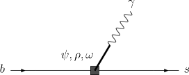
Figure 12: Vector-Meson-Dominance contributions mediated by ${\psi,\rho,\omega}$.

Here we want to discuss the long distance contributions. In order to examine the standard model or search for new physics indirectly by comparing the experimental data with the values predicted within the standard model, we have to take into account these long distance effects: ${B\to K^{*}(J/\psi,\rho,\omega)\rightarrow K^{*}\gamma}$ Golowich:1994zr ; Deshpande:1994cn (Fig.12). It should be noted that ${B\to D\bar{D}K^{*}\to K^{*}\gamma}$ is small compared to the ${J/\psi}$ intermediate state contribution.

These contributions are caused by ${O_{1}}$, ${O_{2}}$ operators, and the effective Hamiltonian describing these processes is

$$H_{eff}=\frac{G_{F}}{\sqrt{2}}\sum_{q=u,c}V_{qb}V_{qs}^{*}(C_{1}(t)O_{1}^{(q)}(t)+C_{2}(t)O_{2}^{(q)}(t))+\mbox{h.c.}$$

If we use the vector-meson-dominance, the ${B\to K^{*}\gamma}$ decay amplitude can be expressed as inserting the complete set of possible intermediate vector meson states like

$$\langle K^{*}\gamma|H_{eff}|B\rangle=\sum_{V}\langle\gamma|A_{\nu}J_{em}^{\nu}|V\rangle\frac{-i}{q_{V}^{2}-m_{V}^{2}}\langle VK^{*}|H_{eff}|B\rangle,$$

where ${V=\psi,\rho,\omega}$. Now we concretely consider the ${B\rightarrow K^{*}\psi\to K^{*}\gamma}$. Four diagrams contribute to the hadronic matrix element of ${\langle K^{*}\psi|H_{eff}|B\rangle}$ (see Fig.13), and first of all, we consider the leading contributions: the factorizable ones, Figs. 13(A) and 13(B).

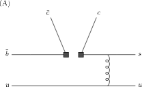
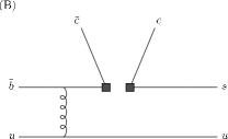
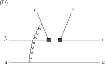
Figure 13: (A), (B) are factorizable and (C), (D) are nonfactorizable contributions to the hadronic matrix element for ${<K^{*}\psi|H_{eff}|B>}$.

V.1 Factorizable contribution

In this case, the ${B\to\psi K^{*}}$ decay amplitude can be factorized as

$$\langle\psi K^{*}\mid H_{eff}\mid B\rangle = \frac{G_{F}}{\sqrt{2}}V_{cb}V_{cs}^{*}a_{1}(t)\langle\psi\mid\bar{c}\gamma_{\mu}(1-\gamma^{5})c\mid 0\rangle$$ (66)

$$\times\langle K^{*}\mid\bar{s}\gamma^{\mu}(1-\gamma^{5})b\mid B\rangle,$$

and the definition of the decay constant is

$$\langle\psi(q)\mid\bar{c}\gamma_{\mu}c\mid 0\rangle\equiv im_{\psi}g_{\psi}(q^{2})\epsilon_{\psi\mu}^{*}(q),$$ (67)

then the decay amplitude can be written as

$$M(B\rightarrow K^{*}\psi(q)) = \frac{G_{F}}{\sqrt{2}}V_{cb}V_{cs}^{*}a_{1}(t)im_{\psi}g_{\psi}(q^{2})\epsilon^{*}_{\psi\mu}(q)$$ (68)

$$\times\langle K^{*}\mid\bar{s}\gamma^{\mu}(1-\gamma^{5})b\mid B\rangle,$$

where ${a_{1}(t)=C_{1}(t)+C_{2}(t)/3}$. The conversion part of the ${\psi}$ meson into photon can be expressed as

$$\langle\gamma\mid A_{\nu}J_{em}^{\nu}\mid\psi\rangle=-\frac{2}{3}em_{\psi}g_{\psi}(q^{2}),$$ (69)

then the total amplitude of ${B\to K^{*}\gamma}$ mediated by ${\psi}$ meson can be expressed as follows,

$$M(B\rightarrow K^{*}\psi\to K^{*}\gamma) = \frac{G_{F}}{\sqrt{2}}V_{cb}V_{cs}^{*}a_{1}(t)\left(\frac{2eg_{\psi}(0)^{2}}{3}\right)\epsilon_{\psi\mu}^{*}$$ (70)

$$\times\langle K^{*}\mid\bar{s}\gamma^{\mu}(1-\gamma^{5})b\mid B\rangle$$

where the real photon momentum is ${q^{2}=0}$. In principle, we need to include the width of the vector meson in the propagator and write

$$\frac{-i}{q^{2}-m^{2}+im\Gamma}~{},$$ (71)

but we have ${(\Gamma_{\psi}/m_{\psi})\sim O(10^{-5})}$ and the effects of the width can be safely neglected.

The amplitudes for ${B\rightarrow K^{*}\omega\rightarrow K^{*}\gamma}$ can be computed in a similar manner. In this case, ${(\Gamma_{\omega}/m_{\omega})=1.0\times 10^{-2}}$ and we can also neglect the width effect in the meson propagator. Differences with ${B\rightarrow K^{*}\psi\rightarrow K^{*}\gamma}$ are the value of decay constant ${g_{\omega}(0)}$ and the factor for the electromagnetic interaction.

$$M(B\rightarrow K^{*}\omega\rightarrow K^{*}\gamma) = \frac{G_{F}}{\sqrt{2}}V_{ub}V_{us}^{*}a_{1}(t)\left(\frac{eg_{\omega}(0)^{2}}{6}\right)\epsilon_{\omega\mu}^{*}$$ (72)

$$\times\langle K^{*}\mid\bar{s}\gamma^{\mu}(1-\gamma^{5})b\mid B\rangle$$

However in the ${B\rightarrow K^{*}\rho\rightarrow K^{*}\gamma}$ case, the ${\rho}$ resonance peak is not so sharp, so the propagation of ${\rho}$ meson generates the strong phase: ${(\Gamma_{\rho}/m_{\rho})\simeq 0.19}$ and it introduces ${\simeq 11^{\circ}}$ strong phase.

$$M(B\rightarrow K^{*}\rho\rightarrow K^{*}\gamma) = \frac{G_{F}}{\sqrt{2}}V_{ub}V_{us}^{*}a_{1}(t)\left(\frac{eg_{\rho}(0)^{2}}{2(1-i\Gamma_{\rho}/m_{\rho})}\right)\epsilon_{\rho\mu}^{*}$$ (73)

$$\times\langle K^{*}\mid\bar{s}\gamma^{\mu}(1-\gamma^{5})b\mid B\rangle$$

In order to estimate these long distance contributions, we have to know the decay constant ${g_{V}}$. The decay constants are experimentally determined by the ${V\rightarrow e^{+}e^{-}}$ data Eidelman:2004wy . The amplitude for ${V\to e^{+}e^{-}}$ can be expressed as

$$M(V\to e^{+}e^{-})=Qe^{2}m_{V}g_{V}(q^{2})$$ (74)

where ${Q}$ expresses the electric charge like that ${Q=Q_{c}}$ when ${V=\psi}$, ${Q=(Q_{u}-Q_{d})/\sqrt{2}}$ in ${V=\rho}$ case, and in ${V={\omega}}$ case, ${Q=(Q_{u}+Q_{d})/\sqrt{2}}$. Then the decay width for ${V\rightarrow e^{+}e^{-}}$ decay can be written like

$$\Gamma(V\rightarrow e^{+}e^{-})=\frac{4\pi Q^{2}\alpha_{em}^{2}g_{V}^{2}(q^{2})}{3m_{V}}~{},$$ (75)

and the values of ${g_{V}}$ are in Table 1.

${V}$	${\Gamma(V\rightarrow e^{+}e^{-})(GeV)}$	${m_{V}(GeV)}$	${g_{V}^{2}(GeV^{2})}$
${J/\psi(1S)}$	${5.26\times 10^{-6}}$	3.097	0.1642
${\psi(2S)}$	${2.19\times 10^{-6}}$	3.686	0.0814
${\psi(3770)}$	${0.26\times 10^{-6}}$	3.770	0.0099
${\psi(4040)}$	${0.75\times 10^{-6}}$	4.040	0.0306
${\psi(4160)}$	${0.77\times 10^{-6}}$	4.160	0.0323
${\psi(4415)}$	${0.47\times 10^{-6}}$	4.415	0.0209
${\rho}$	${7.02\times 10^{-6}}$	0.771	0.0485
${\omega}$	${0.60\times 10^{-6}}$	0.783	0.0379

Table 1: The coefficients ${g_{V}}$.

Furthermore, these decay constants are defined at the ${q^{2}=m_{V}^{2}}$ energy scale. We need ones at ${q^{2}=0}$, so we have to extrapolate these decay constants from ${q^{2}=m_{V}^{2}}$ to ${q^{2}=0}$. We express ${g_{V}(0)}$ as ${g_{V}(0)=\kappa g_{V}(q^{2})}$ by using suppression factor ${\kappa}$. In the ${\psi}$ cases, we take ${\kappa\simeq 0.4}$ Golowich:1994zr ; Deshpande:1994cn , and in the ${\rho,\omega}$ cases, we take ${\kappa\simeq 1.0}$ Anderson:1976hi ; Paul:1981dw . Then the long distance contributions mediated by ${\psi,\rho,\omega}$ are

$$M(B\rightarrow K^{*}\gamma) = \frac{G_{F}}{\sqrt{2}}a_{1}(t)e\Big{(}V_{cb}V_{cs}^{*}\frac{2\kappa g_{\psi}(m_{\psi}^{2})^{2}}{3}+V_{ub}V_{us}^{*}\left[\frac{g_{\omega}(m_{\omega}^{2})^{2}}{6}+\frac{g_{\rho}(m_{\rho}^{2})^{2}}{2(1-i\Gamma/m_{\rho})}\right]\Big{)}\epsilon_{\gamma\mu}\langle K^{*}\mid\bar{s}\gamma^{\mu}(1-\gamma^{5})b\mid B\rangle,$$ (76)

and if we calculate the form factor of ${\langle K^{*}\mid\bar{s}\gamma^{\mu}(1-\gamma^{5})b\mid B\rangle}$, the long distance contributions become as follows:

$$M^{S(A)} = -M^{P(A)}$$ (77)

$$= \frac{8\pi^{2}}{M_{B}^{2}}F^{(0)}\int^{1}_{0}dx_{1}dx_{2}\int b_{1}db_{1}b_{2}db_{2}\phi_{B}(x_{1},b_{1})S_{t}(x_{2})\alpha_{s}(t_{7}^{a})e^{[-S_{B}(t_{7}^{a})-S_{K^{*}}(t_{7}^{a})]}a_{1}(t_{7}^{a})H_{7}^{(a)}(A_{7}b_{2},B_{7}b_{1},B_{7}b_{2})$$

$$\times r_{K^{*}}\left[\phi_{K^{*}}^{v}(x_{2})+\phi_{K^{*}}^{a}(x_{2})\right]\left(\xi_{c}\frac{2\kappa g_{\psi}(m_{\psi}^{2})^{2}}{3}+\xi_{u}\left[\frac{g_{\omega}(m_{\omega}^{2})^{2}}{6}+\frac{g_{\rho}(m_{\rho}^{2})^{2}}{2(1-i\Gamma/m_{\rho})}\right]\right)$$

$$\hskip 85.35826pt\left(t_{7}^{a}=max(A_{7},B_{7},1/b_{1},1/b_{2})\right)$$

$$M^{S(B)} = \frac{8\pi^{2}}{M_{B}^{2}}F^{(0)}\int^{1}_{0}dx_{1}dx_{2}\int b_{1}db_{1}b_{2}db_{2})\phi_{B}(x_{1},b_{1})S_{t}(x_{2})\alpha_{s}(t_{7}^{b})e^{[-S_{B}(t_{7}^{b})-S_{K^{*}}(t_{7}^{b})]}a_{1}(t_{7}^{b})H_{7}^{(b)}(A_{7}b_{1},C_{7}b_{1},C_{7}b_{2})$$

$$\times\Big{[}(x_{2}+2)r_{K^{*}}\phi_{K^{*}}^{v}(x_{2})+\phi_{K^{*}}^{T}(x_{2})-x_{2}r_{K^{*}}\phi_{K^{*}}^{a}(x_{2})\Big{]}\left(\xi_{c}\frac{2\kappa g_{\psi}(m_{\psi}^{2})^{2}}{3}+\xi_{u}\left[\frac{g_{\omega}(m_{\omega}^{2})^{2}}{6}+\frac{g_{\rho}(m_{\rho}^{2})^{2}}{2(1-i\Gamma/m_{\rho})}\right]\right)$$

$$M^{P(B)} = -\frac{8\pi^{2}}{M_{B}^{2}}F^{(0)}\int^{1}_{0}dx_{1}dx_{2}\int b_{1}db_{1}b_{2}db_{2}\phi_{B}(x_{1},b_{1})S_{t}(x_{2})\alpha_{s}(t_{7}^{b})e^{[-S_{B}(t_{7}^{b})-S_{K^{*}}(t_{7}^{b})]}a_{1}(t_{7}^{b})H_{7}^{(b)}(A_{7}b_{1},C_{7}b_{1},C_{7}b_{2})$$ (79)

$$\times\Big{[}-x_{2}r_{K^{*}}\phi_{K^{*}}^{v}(x_{2})+\phi_{K^{*}}^{T}(x_{2})+(x_{2}+2)r_{K^{*}}\phi_{K^{*}}^{a}(x_{2})\Big{]}\left(\xi_{c}\frac{2\kappa g_{\psi}(m_{\psi}^{2})^{2}}{3}+\xi_{u}\left[\frac{g_{\omega}(m_{\omega}^{2})^{2}}{6}+\frac{g_{\rho}(m_{\rho}^{2})^{2}}{2(1-i\Gamma/m_{\rho})}\right]\right)$$

$$\hskip 85.35826pt\left(t_{7}^{b}=max(A_{7},C_{7},1/b_{1},1/b_{2})\right)$$

V.2 Nonfactorizable contribution

Next we estimate the the effect of nonfactorizable contributions to the physical quantity like branching ratio, CP asymmetry, and isospin breaking effects. In order to do so in the case of ${B\to K^{*}\psi\to K^{*}\gamma}$ at first, we use the experimental data on the branching ratio and different helicity amplitudes for ${B\to J/\psi~{}K^{*}}$ decay mode. The branching ratio is ${Br(B^{0}\to J/\psi~{}K^{*0})=(1.31\pm 0.07)\times 10^{-3}}$Eidelman:2004wy , and the fraction of the transversely polarized decay width to the total decay width is about ${\Gamma_{T}/\Gamma=\simeq 0.4}$ Abe:2002ha ; Aubert:2001pe ; Jpsi , then the corresponding transversally polarized branching ratio amounts to

$$Br(B\to J/\psi~{}K^{*})_{T}\simeq 5.0\times 10^{-4}.$$ (80)

On the other hand, if we compute the branching ratio by using eq.(66), we have

$$Br(B\to J/\psi~{}K^{*})_{T}\simeq 2.3\times 10^{-4}.$$ (81)

If we assume that the difference between the experimental value eq.(80) and our prediction eq.(81) is due to the nonfactorizable amplitude, then

$$\frac{\mbox{nonfactorizable}~{}A(B\to J/\psi~{}K^{*})_{T}}{\mbox{factorizable}~{}A(B\to J/\psi~{}K^{*})_{T}}\simeq 0.4~{}.$$ (82)

Note however, that ${B\to K^{*}\gamma}$ is dominated by the short distance amplitudes. The long distance correction from the factorizable diagram is about 4% of the total decay amplitude. So when we add the nonfactorizable amplitude, the long distance correction increases to 6% in the total amplitude, and 12% in the branching ratio. We have included these corrections in our numerical estimates given below.

Furthermore, we estimate the effect of nonfactorizable contribution to the direct CP asymmetry. In general, a nonfactorized amplitudes has a relative strong phase compared to the factorized amplitude. We already know that the nonfactorizable diagram amounts to about 2% to the short distance amplitude, then we can numerically estimate the CP asymmetry uncertainty from the nonfactorizable diagram by introducing the strong phase as a free parameter. We conclude that only less than 10% uncertainty is generated by the long distance nonfactorizable amplitude, and as we will see later, this error is small compared to the total uncertainty in CP asymmetry from other origins. Finally, we mention that these long distance contributions do not generate the isospin breaking effect, the nonfactorizable contribution can be neglected in computing the isospin breaking effects.

In the case of ${B\to K^{*}(\rho,\omega)\to K^{*}\gamma}$, we can expect that the factorized amplitudes are dominant to the total decay amplitude in ${B\to K^{*}(\rho,\omega)}$ by the analogy of ${B\to\rho\rho}$ decay Kagan:2004uw , then we can neglect the nonfactorized contribution to the above physical quantities.

V.3 Another diagrams for long distance contributions to the photon quark coupling

Next we want to consider another contribution with different topology which exist only in the charged decay mode like ${B^{\pm}\to K^{*\pm}\gamma}$ (Fig.14). If we neglect the nonfactorizable contributions and annihilation contributions, there are two diagrams that contribute to the hadronic matrix elements ${\langle K^{*\pm}\rho(\omega)\mid H_{eff}\mid B^{\pm}\rangle}$.

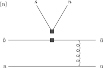
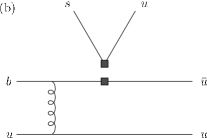
Figure 14: Long distance effects mediated by ${\rho,\omega}$ which contribute only to the charged mode.

We define the ${\rho}$ or ${\omega}$ meson momentum ${P_{3}=M_{B}/\sqrt{2}\hskip 2.84526pt(1,0,\vec{0}_{T})}$ and the spectator quark momentum fraction as ${x_{3}}$.

$$M^{S(a)} = -M^{P(a)}$$ (83)

$$= \frac{4\pi^{2}f_{K^{*}}}{M_{B}^{2}}F^{(0)}\xi_{u}\int^{1}_{0}dx_{1}dx_{3}\int b_{1}db_{1}b_{3}db_{3}~{}\phi_{B}(x_{1},b_{1})\Big{[}\frac{g_{\rho}(m_{\rho}^{2})}{1-i\Gamma/m_{\rho}}+\frac{g_{\omega}(m_{\omega}^{2})}{3}\Big{]}S_{t}(x_{1})\alpha_{s}(t^{a})e^{\left[-S_{B}(t^{a})-S_{\rho}(t^{a})\right]}$$

$$\times a_{2}(t^{a})r_{\rho}\left[\phi_{\rho}^{v}(x_{3})+\phi_{\rho}^{a}(x_{3})\right]H_{7}^{(a)}(A_{7}b_{3},B_{7}b_{1},B_{7}b_{3})\hskip 14.22636pt\left(t^{a}=\mbox{max}(A_{7},B_{7},1/b_{1},1/b_{3})\right)$$

$$M^{S(b)} = \frac{4\pi^{2}f_{K^{*}}}{M_{B}^{2}}F^{(0)}\xi_{u}\int^{1}_{0}dx_{1}dx_{3}\int b_{1}db_{1}b_{3}db_{3}~{}\phi_{B}(x_{1},b_{1})\Big{[}\frac{g_{\rho}(m_{\rho}^{2})}{1-i\Gamma/m_{\rho}}+\frac{g_{\omega}(m_{\omega}^{2})}{3}\Big{]}S_{t}(x_{2})\alpha_{s}(t^{b})e^{\left[-S_{B}(t^{b})-S_{\rho}(t^{b})\right]}$$ (84)

$$\times a_{2}(t^{b})\left[(x_{3}+2)r_{\rho}\phi_{\rho}^{v}(x_{3})+\phi_{\rho}^{T}(x_{3})-x_{3}r_{\rho}\phi_{\rho}^{a}(x_{3})\right]H_{7}^{(b)}(A_{7}b_{1},C_{7}b_{1},C_{7}b_{3})$$

$$M^{P(b)} = -\frac{4\pi^{2}f_{K^{*}}}{M_{B}^{2}}F^{(0)}\xi_{u}\int^{1}_{0}dx_{1}dx_{3}\int b_{1}db_{1}b_{3}db_{3}~{}\phi_{B}(x_{1},b_{1})\Big{[}\frac{g_{\rho}(m_{\rho}^{2})}{1-i\Gamma/m_{\rho}}+\frac{g_{\omega}(m_{\omega}^{2})}{3}\Big{]}S_{t}(x_{2})\alpha_{s}(t^{b})e^{\left[-S_{B}(t^{b})-S_{\rho}(t^{b})\right]}$$ (85)

$$\times a_{2}(t^{b})\left[-x_{3}r_{\rho}\phi_{\rho}^{v}(x_{3})+\phi_{\rho}^{T}(x_{3})+(x_{3}+2)r_{\rho}\phi_{\rho}^{a}(x_{3})\right]H_{7}^{(b)}(A_{7}b_{1},C_{7}b_{1},C_{7}b_{3})$$

$$\hskip 85.35826pt\left(t^{b}=\mbox{max}(A_{7},C_{7},1/b_{1},1/b_{3})\right)$$

$$A_{7}^{2}=x_{1}x_{3}M_{B}^{2},\hskip 17.07164ptB_{7}^{2}=x_{1}M_{B}^{2},\hskip 17.07164ptC_{7}^{2}=x_{3}M_{B}^{2}$$ (86)

In the computation of the above formulas, we use the ${\rho}$ and ${\omega}$ meson wave function extracted from light-cone QCD sum rule Ball:1998ff , and the detailed expression is in Appendix C.

VI Numerical results

We want to show the numerical analysis in this section. In the evaluation of the various form factors and amplitudes, we adopt ${G_{F}=1.16639\times 10^{-5}\mbox{GeV}^{-2}}$, leading order strong coupling ${\alpha_{s}}$ defined at the flavor number ${n_{f}=4}$, the decay constants ${f_{B}=190\mbox{MeV}}$, ${f_{K^{*}}=226\mbox{MeV}}$, and ${f_{K^{*}}^{T}=185\mbox{MeV}}$, the masses ${M_{B}=5.28\mbox{GeV}}$, ${M_{K^{*}}=0.892\mbox{GeV}}$ and ${m_{c}=1.2\mbox{GeV}}$, the meson lifetime ${\tau_{B^{0}}=1.542\hskip 2.84526pt\mbox{ps}}$ and ${\tau_{B^{+}}=1.674\hskip 2.84526pt\mbox{ps}}$. Furthermore we used the leading order Wilson coefficients Buchalla:1995vs and we take the ${K^{*}}$, ${\rho}$, and ${\omega}$ meson wave functions up to twist-3. In order to make clear the theoretical error of the predicted physical quantities, we want to show how to estimate these errors.

VI.1 Error Estimation

When we estimate the physical quantities like branching ratio, CP asymmetry, and isospin breaking effect, there are four major classes of error in pQCD computations: (1) the input parameter uncertainties; (2) higher order effects in perturbation expansion; (3) the CKM parameter uncertainties; and (4) the hadronic uncertainties from the ${u}$ quark loop.

1. First we want to estimate the class(1) error for various physical quantities. For class(1), we change the decay constants, the B meson wave function parameter ${\omega_{B}}$, and ${c}$ parameter of the threshold function. We estimate the uncertainties from the decay constants to be 15% in the amplitude. If we change the ${\omega_{B}}$ in the range ${\omega_{B}=(0.40\pm 0.04)}$GeV, and ${c}$ in the range ${c=0.4\pm 0.1}$, these uncertainties change the ${B\to K^{*}}$ form factor by about 15% at the amplitude level. Thus we regard the total uncertainty for class(1) to be 20%. Here we discuss how this error affects the experimental observables such as the branching ratio, direct CP asymmetry, and isospin breaking.

   • Branching Ratio

     In order to see how much error is generated when we change some parameters in class(1), we introduce real parameter ${\delta_{i}^{j}}$’s as the fractional differences of the amplitudes from ones with a fixed hadronic parameter, where ${i}$ and ${j}$ express the flavor and electric charge. Note that the uncertainty in decay constants leads to an uncertainty in overall factor of the amplitude, i.e. they don’t lead to an uncertainty in the phase of the amplitude. In the change wave function parameters on the other hand, the phase changes a little, but it’s effect is very small and we can introduce ${\delta_{i}^{j}}$’s as real parameters.

     The decay widths of the ${B}$ and ${\bar{B}}$ meson decays can be expressed as

     $$\Gamma({B}^{j}) = |V_{tb}^{*}V_{ts}A_{t}^{j}(1+\delta_{t}^{j})+V_{cb}^{*}V_{cs}A_{c}^{j}(1+\delta_{c}^{j})+V_{ub}^{*}V_{us}A_{u}^{j}(1+\delta_{u}^{j})|^{2}$$ (87)

     $$\Gamma(\bar{B}^{j}) = |V_{tb}V_{ts}^{*}A_{t}^{j}(1+\delta_{t}^{j})+V_{cb}V_{cs}^{*}A_{c}^{j}(1+\delta_{c}^{j})+V_{ub}V_{us}^{*}A_{u}^{j}(1+\delta_{u}^{j})|^{2},$$ (88)

     and we can see that the uncertainty to the branching ratio from input parameters comes from the error of the ${O_{7\gamma}}$ amplitude, and it amounts to about ${2\delta_{t}^{j}\simeq 40\%}$.

   • Direct CP Asymmetry

     From eq.(87) and (88), the direct CP asymmetry can be expressed as follows,

     $$A_{CP}^{\prime} = \frac{2}{|V_{tb}^{*}V_{ts}|^{2}|A_{t}^{j}|^{2}(1+\delta_{t}^{j})}\Big{[}Im(V_{tb}^{*}V_{ts}V_{cb}V_{cs}^{*})Im(A_{t}^{j}A_{c}^{*j})(1+\delta_{c}^{j})+Im(V_{tb}^{*}V_{ts}V_{ub}V_{us}^{*})Im(A_{t}^{j}A_{u}^{*j})(1+\delta_{u}^{j})\Big{]}$$ (89)

     and the error for it is

     $$\frac{\Delta A_{CP}}{A_{CP}}=\frac{A_{CP}^{\prime}-A_{CP}}{A_{CP}}\propto\frac{(\delta_{c}^{j}-\delta_{t}^{j})Im(A_{c}^{j*}/A_{t}^{j*})+(\delta_{u}^{j}-\delta_{t}^{j})Im(A_{u}^{j*}/A_{t}^{j*})}{(1+\delta_{t}^{j})[Im(A_{c}^{j*}/A_{t}^{j*})+Im(A_{u}^{j*}/A_{t}^{j*})]}~{}.$$ (90)

     We can see that the uncertainties can cancel. We have checked that numerically the class(1) error for the CP asymmetry amounts to few percent and is small compared to other errors (see below).

   • Isospin Breaking

     On the other hand, we want to show that the hadronic parameter uncertainties especially from ${\omega_{B}}$ and ${c}$ dependences of the isospin breaking effect can be large even though we take the ratio as the CP asymmetry. The decay width of the neutral and charged decay modes with the theoretical error can be written from eq.(87) and (88) as

     $$\Gamma^{0} = |V_{tb}^{*}V_{ts}A_{t}^{0}(1+\delta_{t}^{0})+V_{cb}^{*}V_{cs}A_{c}^{0}(1+\delta_{c}^{0})+V_{ub}^{*}V_{us}A_{u}^{0}(1+\delta_{u}^{0})|^{2},$$ (91)

     $$\Gamma^{+} = |V_{tb}^{*}V_{ts}A_{t}^{+}(1+\delta_{t}^{+})+V_{cb}^{*}V_{cs}A_{c}^{+}(1+\delta_{c}^{+})+V_{ub}^{*}V_{us}A_{u}^{+}(1+\delta_{u}^{+})|^{2},$$ (92)

     and the isospin breaking effect is given by

     $$\Delta_{0+}^{\prime}=\frac{|A_{t}^{0}|^{2}(1+\delta_{t}^{0})^{2}-|A_{t}^{+}|^{2}(1+\delta_{t}^{+})^{2}}{|A_{t}^{0}|^{2}(1+\delta_{t}^{0})^{2}+|A_{t}^{+}|^{2}(1+\delta_{t}^{+})^{2}}~{},$$ (93)

     where we neglected all terms except for those proportional to ${|A_{t}^{j}|^{2}}$ because ${|A_{c}^{j}|^{2}/|A_{t}^{j}|^{2}\sim O(10^{-4})}$, and the CKM factor of the ${|A_{u}^{j}|^{2}}$ is suppressed as ${|V_{ub}V_{us}^{*}/V_{tb}^{*}V_{ts}|^{2}\sim O(\lambda^{4})}$. Then the error can be expressed as

     $$\frac{\Delta(\Delta_{0+})}{\Delta_{0+}}=\frac{\Delta_{0+}^{\prime}-\Delta_{0+}}{\Delta_{0+}}\approx\frac{4|A_{t}^{0}|^{2}|A_{t}^{+}|^{2}\Big{[}\delta_{t}^{0}-\delta_{t}^{+}\Big{]}}{(|A_{t}^{0}|^{2}-|A_{t}^{+}|^{2})(|A_{t}^{0}|^{2}+|A_{t}^{+}|^{2})}~{}.$$ (94)

     We can easily imagine that the decay constant uncertainties are canceled as the direct CP asymmetry. However we observe that even though ${\delta_{t}^{0}-\delta_{t}^{+}}$ is small, there exist ${|A_{t}^{0}|^{2}-|A_{t}^{+}|^{2}}$ in the denominator and it is also small, then the error enhancement can occur. Variation of ${\omega_{B}}$ and ${c}$ introduces ${\delta_{t}^{0}-\delta_{t}^{+}\simeq 0.5\%}$ while ${(|A_{t}^{0}|^{2}-|A_{t}^{+}|^{2})/(|A_{t}^{0}|^{2}+|A_{t}^{+}|^{2})\simeq 5\%}$. This gives about 20% error for the isospin breaking. From the above argument, we can see that the error from ${\omega_{B}}$ and ${c}$ uncertainties remain somewhat large. Thus we estimate the class(1) error for the isospin breaking effect to be about 20%.

2. Next we want to discuss the class(2) error. For class(2), we expect an error coming from the fact that we used the leading order term in ${\alpha_{s}(t)}$. There are also errors coming from neglecting higher order decay amplitudes. But we have not checked the effect of class(2) errors as it requires actual computation of higher order amplitudes. We guess that the error is approximately 15% in the amplitude. Then the theoretical errors from class(2) are 30% in the branching ratio, about a few % in the direct CP asymmetry, and 20% in the isospin breaking effect.

3. About the class(3) error, we change the ${\bar{\rho}}$, ${\bar{\eta}}$ parameter in the range ${\bar{\rho}=\rho(1-\lambda^{2}/2)}$ ${=0.20\pm 0.09}$ and ${\bar{\eta}=\eta(1-\lambda^{2}/2)=0.33\pm 0.05}$ Eidelman:2004wy , and numerically estimate how the physical quantities are affected by the changing of parameters. The major contributions to the branching ratio and isospin breaking effects come from the terms which are proportional to ${V_{tb}^{*}V_{ts}}$, so they are less sensitive to the error in ${\bar{\rho}}$, ${\bar{\eta}}$. On the other hand, direct CP asymmetry depends on ${Im(V_{tb}^{*}V_{ts}V_{cb}V_{cs}^{*})}$ and ${Im(V_{tb}^{*}V_{ts}V_{ub}V_{us}^{*})}$ as in eq.(89), thus the error from the ${\bar{\rho}}$, ${\bar{\eta}}$ uncertainties amounts to about 15%.

4. The class(4) error comes from the ${u}$ quark loop hadronic uncertainties. The terms which are proportional to ${V_{ub}^{*}V_{us}}$ are not very important to the computation of the branching ratio and isospin breaking effect, so for these quantities we can neglect the class(4) uncertainties.

   However for CP asymmetry, ${c}$ and ${u}$ quark loops give comparable contributions as seen in eq.(89), thus the ${u}$ quark loop contribution which is infected with nonperturbative correction, cannot be neglected. If we regard the ${u}$ quark loop uncertainty as about 100% at the amplitude level for both real and imaginary part, the numerical error for the direct CP asymmetry amounts to about 75%.

In summary, we regard the error of the branching ratio, direct CP asymmetry, and isospin breaking effects as 50% (class(1); 40%, class(2); 30%), 75% (class(4); 75%), and 30% (class(1); 20%, class(2); 20%), respectively.

VI.2 Numerical Results

The numerical results for each decay amplitude ${M_{i}}$ in the neutral decay (Table2) and charged decay (Table3) in unit of ${10^{-6}\mbox{GeV}^{-2}}$ are as follows.

The total decay amplitude can be expressed by using these components as

$$A(B\to K^{*}\gamma) = M_{t}+M_{c}+M_{u}$$ (95)

$$= (\epsilon_{\gamma}^{*}\cdot\epsilon_{K^{*}}^{*})(M_{t}^{S}+M_{c}^{S}+M_{u}^{S})$$

$$+ i\epsilon_{\mu\nu+-}\epsilon_{\gamma}^{*\mu}\epsilon_{K^{*}}^{*\nu}(M_{t}^{P}+M_{c}^{P}+M_{u}^{P}),$$

$$M_{t} = M_{7\gamma}+M_{8g}+M_{3\sim 6},$$

$$M_{c} = M_{1c}+M_{2c}+M_{\psi},$$

$$M_{u} = M_{1u+2u}+M_{2}+M_{\rho+\omega},$$

where all components include CKM factors. If we express ${K^{*}}$ and ${\gamma}$ helicities as ${\lambda_{1},\lambda_{2}}$, the combinations which can contribute to the decay amplitude are ${A_{\lambda_{1},\lambda_{2}}=A_{+,+},A_{-,-}}$, if we take into account the fact that ${B}$ meson is spinless and a real photon has helicities ${\pm 1}$. Then the total decay width of ${B\to K^{*}\gamma}$ is given by

$$\Gamma=\frac{1}{8\pi M_{B}}\left(|M_{t}^{S}+M_{c}^{S}+M_{u}^{S}|^{2}+|M_{t}^{P}+M_{c}^{P}+M_{u}^{P}|^{2}\right),\hskip 5.69054pt$$ (96)

and the branching ratios for ${B\to K^{*}\gamma}$ become as follows:

$$Br(B^{0}\to K^{*0}\gamma) = (5.8\pm 2.9)\times 10^{-5},$$ (97)

$$Br(B^{\pm}\to K^{*\pm}\gamma) = (6.0\pm 3.0)\times 10^{-5}.$$ (98)

Next we want to extract the direct CP asymmetry. We take into account up to ${O(\lambda^{4})}$ about the CKM matrix components,

$$\footnotesize{V_{KM}}=$$

$$\begin{pmatrix}\footnotesize{1-\lambda^{2}/2-\frac{\lambda^{4}}{8}}&\footnotesize{\lambda}&\footnotesize{A{{\lambda}^{3}}(\rho-i\eta)}\\ \footnotesize{-\lambda}&\footnotesize{1-\lambda^{2}/2-\left(1/8+A^{2}/2\right)\lambda^{4}}&\footnotesize{A{{\lambda}^{2}}}\\ \footnotesize{A{{\lambda}^{3}}(1-\rho-i\eta)}&\footnotesize{-A\lambda^{2}+A\lambda^{4}\left(1/2-\rho-i\eta\right)}&\footnotesize{1-A^{2}\lambda^{4}/2}\end{pmatrix}$$

and the unitary triangle related to this decay mode should be crushed (Fig.15).

Figure 15: CKM unitary triangle

If we express each amplitudes ${M_{i}}$ as ${\xi_{i}A_{i}e^{i\delta_{i}}}$ where ${\xi_{i}=V_{ib}^{*}V_{is}/V_{cb}^{*}V_{cs}}$, in order to separate weak phase and strong phase ${\delta_{i}}$, the decay amplitudes can be rewritten as

$$A(B\to K^{*}\gamma)=V_{cb}^{*}V_{cs}\hskip 2.84526pt[\xi_{t}A_{t}e^{i\delta_{t}}+\xi_{c}A_{c}e^{i\delta_{c}}+\xi_{u}A_{u}e^{i\delta_{u}}],$$ (100)

$$A(\bar{B}\to\bar{K^{*}}\gamma)=V_{cb}V_{cs}^{*}\hskip 2.84526pt[\xi_{t}^{*}A_{t}e^{i\delta_{t}}+\xi_{c}^{*}A_{c}e^{i\delta_{c}}+\xi_{u}^{*}A_{u}e^{i\delta_{u}}],$$ (101)

and the direct CP asymmetry can be expressed as

$$A_{CP}\equiv\frac{\Gamma(\bar{B}\to\bar{K^{*}}\gamma)-\Gamma(B\to K^{*}\gamma)}{\Gamma(\bar{B}\to\bar{K^{*}}\gamma)+\Gamma(B\to K^{*}\gamma)}\equiv\frac{R_{N}}{R_{D}},$$ (102)

$$R_{N} = \Big{[}A_{t}A_{c}\sin(\delta_{t}-\delta_{c})\mbox{Im}(V_{tb}V_{ts}^{*}V_{cb}^{*}V_{cs})$$ (103)

$$\hskip 14.22636pt+A_{c}A_{u}\sin(\delta_{c}-\delta_{u})\mbox{Im}(V_{cb}V_{cs}^{*}V_{ub}^{*}V_{us})$$

$$\hskip 14.22636pt+A_{u}A_{t}\sin(\delta_{u}-\delta_{t})\mbox{Im}(V_{ub}V_{us}^{*}V_{tb}^{*}V_{ts})\Big{]},$$

$$R_{D} = \left(A_{t}^{2}|V_{tb}V_{ts}^{*}|^{2}+A_{c}^{2}|V_{cb}V_{cs}^{*}|^{2}+A_{u}^{2}|V_{ub}V_{us}^{*}|^{2}\right)/2$$ (104)

$$\hskip 14.22636pt+A_{t}A_{c}\cos(\delta_{t}-\delta_{c})\mbox{Re}(V_{tb}V_{ts}^{*}V_{cb}^{*}V_{cs})$$

$$\hskip 14.22636pt+A_{c}A_{u}\cos(\delta_{c}-\delta_{u})\mbox{Re}(V_{cb}V_{cs}^{*}V_{ub}^{*}V_{us})$$

$$\hskip 14.22636pt+A_{u}A_{t}\cos(\delta_{u}-\delta_{t})\mbox{Re}(V_{ub}V_{us}^{*}V_{cb}^{*}V_{cs}),$$

then its’ values are

$$A_{CP}(B^{0}\to K^{*0}\gamma) = -(6.1\pm 4.6)\times 10^{-3},$$ (105)

$$A_{CP}(B^{\pm}\to K^{*\pm}\gamma) = -(5.7\pm 4.3)\times 10^{-3}.$$ (106)

Finally, we want to estimate the isospin breaking effects as eq.(I). This effect is caused by ${O_{8g}}$ (Fig.4), ${c}$ and ${u}$ loop contributions (Fig.5), ${O_{1}\sim O_{6}}$ annihilation (Figs.10 and 11), and the long distance contributions mediated ${\rho}$ and ${\omega}$ in charged mode (Fig.14). About the bremsstrahlung photon contributions emitted through quark lines, whether the spectator quark is ${u}$ or ${d}$ affects the strength and the sign for the coupling of photon and quark line, so they generate the isospin breaking effects. The most important contributions to the isospin breaking effects come from QCD penguin ${O_{5}}$, ${O_{6}}$ annihilation. These effects are additive to the dominant contribution ${O_{7\gamma}}$ in both neutral and charged decays (see Tables 2 and 3). However its’ size are different: the neutral mode’s is larger than charged mode’s. Then the sign of total isospin breaking effects becomes plus and it’s value is as follows.

$$\Delta_{0+}=+(2.7\pm 0.8)\times 10^{-2}$$ (107)

		${M_{i}^{S}/F^{(0)}}$			${M_{i}^{P}/F^{(0)}}$
${V_{tb}^{*}V_{ts}}$	${M_{7\gamma}^{S}/F^{(0)}}$	${M_{8g}^{S}/F^{(0)}}$	${M_{3\sim 6}^{S}/F^{(0)}}$	${M_{7\gamma}^{P}/F^{(0)}}$	${M_{8g}^{P}/F^{(0)}}$	${M_{3\sim 6}^{P}/F^{(0)}}$
	-218.67-3.86i	-2.19-0.55i	-11.56-5.70i	218.67+3.86i	2.27+0.59i	11.58+5.63i
${V_{cb}^{*}V_{cs}}$	${M_{1c}^{S}/F^{(0)}}$	${M_{2c}^{S}/F^{(0)}}$	${M_{\psi}^{S}/F^{(0)}}$	${M_{1c}^{P}/F^{(0)}}$	${M_{2c}^{P}/F^{(0)}}$	${M_{\psi}^{P}/F^{(0)}}$
	-0.29-1.01i	6.42-12.63i	-13.29	-0.19+1.27i	-4.81+8.23i	15.09
${V_{ub}^{*}V_{us}}$	${M_{1u+2u}^{S}/F^{(0)}}$	${M_{2}^{S}/F^{(0)}}$	${M_{\rho+\omega}^{S}/F^{(0)}}$	${M_{1u+2u}^{P}/F^{(0)}}$	${M_{2}^{P}/F^{(0)}}$	${M_{\rho+\omega}^{P}/F^{(0)}}$
	-0.63+0.22i	0	-0.03-0.06i	0.67-0.18i	0	0.03+0.07i

Table 2: ${B^{0}\to K^{*0}\gamma}$  at ${\bar{\rho}=0.20}$, ${\bar{\eta}=0.33}$, ${\omega_{B}=0.40\mbox{GeV}}$.

		${M_{i}^{S}/F^{(0)}}$			${M_{i}^{P}/F^{(0)}}$
${V_{tb}^{*}V_{ts}}$	${M_{7\gamma}^{S}/F^{(0)}}$	${M_{8g}^{S}/F^{(0)}}$	${M_{3\sim 6}^{S}/F^{(0)}}$	${M_{7\gamma}^{P}/F^{(0)}}$	${M_{8g}^{P}/F^{(0)}}$	${M_{3\sim 6}^{P}/F^{(0)}}$
	-218.67-3.86i	-4.89-0.10i	-2.47+0.37i	218.67+3.86i	4.83-0.82i	2.86+0.14i
${V_{cb}^{*}V_{cs}}$	${M_{1c}^{S}/F^{(0)}}$	${M_{2c}^{S}/F^{(0)}}$	${M_{\psi}^{S}/F^{(0)}}$	${M_{1c}^{P}/F^{(0)}}$	${M_{2c}^{P}/F^{(0)}}$	${M_{\psi}^{P}/F^{(0)}}$
	-0.66+2.15i	6.42-12.63i	-13.29	1.39-2.60i	-4.81+8.23i	15.09
${V_{ub}^{*}V_{us}}$	${M_{1u+2u}^{S}/F^{(0)}}$	${M_{2}^{S}/F^{(0)}}$	${M_{\rho+\omega}^{S}/F^{(0)}}$	${M_{1u+2u}^{P}/F^{(0)}}$	${M_{2}^{P}/F^{(0)}}$	${M_{\rho+\omega}^{P}/F^{(0)}}$
	-0.75+0.51i	0.35+1.01i	-0.04+0.05i	0.79-0.18i	-0.75+1.16i	0.05-0.05i

Table 3: ${B^{+}\to K^{*+}\gamma}$   at ${\bar{\rho}=0.20}$, ${\bar{\eta}=0.33}$, ${\omega_{B}=0.40\mbox{GeV}}$.

VII Conclusion

In this paper, we calculated the branching ratio, direct CP asymmetry, and isospin breaking effect within the standard model using the pQCD approach. It is useful to compare our results with those existing in the literature. The decay amplitude can be obtained from the transition form factor

$$\langle K^{*}(P_{2},\epsilon_{K^{*}})\mid iq^{\nu}\bar{s}\sigma_{\mu\nu}b\mid B(P_{1})\rangle$$

$$\hskip 56.9055pt=-iT_{1}^{K^{*}}(0)\epsilon_{\mu\alpha\beta\rho}\epsilon_{K^{*}}^{\alpha}P^{\beta}q^{\rho}$$ (108)

where ${P=P_{1}+P_{2}}$, ${q=P_{1}-P_{2}}$. Within the framework of pQCD, we obtain the value of the ${B\to K^{*}}$ transition form factor as ${T_{1}^{K^{*}}(0)=0.23\pm 0.06}$. The result can be compared with the ones extracted by another estimation. In the QCD Factorization, ${T_{1}^{K^{*}}(0)=0.27\pm 0.04}$ Beneke:2001at and an updated phenomenological estimate of this quantity with the light-cone distribution amplitudes for the ${K^{*}}$ meson is ${T_{1}^{K^{*}}(0)=0.27\pm 0.02}$ Ali:2004hn . While the central value in the updated result is the same as before, the error is reduced by a factor of 2. In the light-cone QCD sum rule ${T_{1}^{K^{*}}(0)=0.38\pm 0.06}$ Ball:1998kk , the lattice QCD simulation ${T_{1}^{K^{*}}(0)=0.32^{+0.04}_{-0.02}}$ DelDebbio:1997kr and ${T_{1}^{K^{*}}(0)=0.25^{+0.05}_{-0.02}}$ Becirevic , and the covariant light-front approach ${T_{1}^{K^{*}}(0)=0.24}$ Cheng:2004yj . There are several estimates of the branching ratio by using the value of ${T_{1}^{K^{*}}(0)=0.38\pm 0.06}$ extracted from light-cone QCD sum rule. Comparing the results with experiments, this value of the form factor over estimates the branching ratios Ali:2001ez ; Bosch:2002bw ; Bosch:2001gv . Also, it should be noted that ${T_{1}^{K^{*}}(q^{2})}$ and other related form factors have been computed in the frame work of pQCD Chen:2002bq . They obtained the central value as ${T_{1}^{K^{*}}(0)=0.315}$. The difference between our results and their’s is the ${K^{*}}$ meson wave function. We take the new ${K^{*}}$ wave function parameters computed in Ref.Ball:2003sc .

Note that we have also included the long distance contributions. If we neglect them, the branching ratios become ${Br(B^{0}\to K^{*0}\gamma)=(5.2\pm 2.6)\times 10^{-5}}$ and ${Br(B^{\pm}\to K^{*\pm}\gamma)=(5.3\pm 2.7)\times 10^{-5}}$ to be pared with results shown in Eq.(97) and (98). The ${B\to K^{*}\psi\to K^{*}\gamma}$ contribution to the total decay width amounts to about ${12\%}$ and also it works additive to the branching ratios. We also emphasize that we can calculate the annihilation contributions with the pQCD approach, and these contribute to the total decay width which amount to about ${2\sim 10\%}$.

This analysis predicts less than 1% direct CP asymmetry within the standard model. If we neglect the long distance contributions, the asymmetries become ${A_{CP}(B^{0}\to K^{*0}\gamma)=-(6.7\pm 5.0)\times 10^{-3}}$ and ${A_{CP}(B^{\pm}\to K^{*\pm}\gamma)=-(7.2\pm 5.4)\times 10^{-3}}$, and as to isospin breaking effect like ${\Delta_{0+}=+(2.6\pm 0.8)\times 10^{-2}}$. The long distance contributions do not seem to affect to these asymmetries.

The branching ratio of the neutral decay is similar to that of the charged decay, in spite of the difference of the lifetime between them. This effect is mainly caused by the 4-quark penguin operators ${O_{5}}$, ${O_{6}}$. If we neglect these contributions, the isospin breaking is ${\Delta_{0+}=-(1.2\pm 0.4)\times 10^{-2}}$, so we can see that they generate about 4% isospin breaking effect. This result is similar to the conclusion of Ref.Kagan:2001zk .

${B\to K^{*}\gamma}$ decay, as we have first mentioned, is an attractive decay mode to test the standard model and search for new physics. In order to look for the new physics, we have to reduce the experimental errors. The error to the direct CP asymmetry must get smaller than ${1\%}$. That is to say, we need at least 20 times more data. This is not possible without the super B factory.

Appendix A Brief review of pQCD

A.1 Divergences in perturbative diagrams

Here we want to review the ${k_{T}}$ factorization Nagashima:2002ia . At higher order, infinitely many gluon exchanges must be considered. In order to understand the factorization procedure, we refer to the diagrams of Fig.16.

Figure 16: ${O(\alpha_{s})}$ corrections to the hard scattering ${H}$.

They describe the ${O(\alpha_{s})}$ radiative corrections to the hard scattering process ${H}$. In general, individual higher order diagrams have two types of infrared divergences: soft and collinear. Soft divergence comes from the region of a loop momentum where all it’s momentum components in the light-cone coordinate vanish:

$$l^{\mu}=(l^{+},l^{-},\vec{l}_{T})=(\Lambda,\Lambda,\vec{\Lambda}).$$ (109)

Collinear divergence originates from the gluon momentum region which is parallel to the massless quark momentum,

$$l^{\mu}=(l^{+},l^{-},\vec{l}_{T})\sim(M_{B},\bar{\Lambda}^{2}/M_{B},\vec{\Lambda}).$$ (110)

In both cases, the loop integration correspond to ${\int d^{4}l\hskip 2.84526pt1/l^{4}\sim\log{\Lambda}}$, so logarithmic divergences are generated. It has been shown order by order in perturbation theory that these divergences can be separated from hard kernel and absorbed into meson wave functions using eikonal approximation Li:1994iu .

Furthermore, there are also double logarithm divergences in Fig.16(a) and 16(b) when soft and collinear momentum overlap. These large double logarithm can be summed by using renormalization group equation. This factor is called the Sudakov factor and also factorized into the definition of meson wave function Collins:1981uk ; Botts:kf ; Li:1992nu . The explicit expression for Sudakov factor is given by Botts:kf (see Appendix B).

There are also ultraviolet divergences, and also another type of double logarithm which comes from the loop correction for the weak decay vertex correction. These double logarithm can also be factored out from hard part and grouped into the quark jet function. These double logarithms also should be resumed as the threshold factor Li:2001ay ; Kurimoto:2001zj . This factor decreases faster than any other power of ${x}$ as ${x\rightarrow 0}$, so it removes the endpoint singularity. Thus we can factor out the Sudakov factor, the threshold factor, and the ultraviolet divergences from hard part and grouped into meson wave function (Appendix B). Then the redefinition of wave functions including these loop corrections get factorization energy scale dependence ${t}$.

Thus the amplitude can be factorized into a perturbative part including a hard gluon exchange, and a nonperturbative part characterized by the meson distribution amplitudes. Then the total decay amplitude can be expressed as the convolution:

$$\int^{1}_{0}dx_{1}dx_{2}\int^{1/\Lambda}_{0}d^{2}b_{1}d^{2}b_{2}\hskip 2.84526ptC(t)\otimes\Phi_{K^{*}}(x_{2},b_{2},t)$$

$$\hskip 28.45274pt\otimes H(x_{1},x_{2},b_{1},b_{2},t)\otimes\Phi_{B}(x_{1},b_{1},t),$$ (111)

here ${\Phi_{K^{*}}(x_{2},b_{2},t)}$, ${\Phi_{B}(x_{1},b_{1},t)}$ are meson distribution amplitudes that contain the soft divergences which come from quantum correction and ${H(x_{1},x_{2},b_{1},b_{2},t)}$ is the hard kernel including finite piece of quantum correction, where ${b_{1}}$, ${b_{2}}$ are the conjugate variables to transverse momentum, and ${x_{1}}$, ${x_{2}}$ are the momentum fractions of spectator quarks.

A.2 Physical interpretation of Sudakov factor

In order to understand the Sudakov factor physically, first we consider QED. When a charged particle is accelerated, infinitely many photons must be emitted by the bremsstrahlung (Fig.17(a)).

(a)

(b)

Figure 17: An electron which is scattered by the electromagnetic interaction (a) is observed with many soft photons. Similarly, a quark which is scattered by the strong interaction (b) is not observed as a single gluon: accompanied by many soft gluons, and they form hadron jets.

A similar phenomenon occurs when a quark is accelerated: infinitely many gluons must be emitted. According to the feature of strong interaction, gluons cannot exist freely, so hadronic jet is produced. Then we observe many hadrons in the end if gluonic bremsstrahlung occurs. Thus the amplitude for an exclusive decay ${B\to K^{*}\gamma}$ is proportional to the probability that no bremsstrahlung gluon is emitted. This is the Sudakov factor and it is depicted in Fig.19. As seen in Fig.19, the Sudakov factor is large for small ${b}$ and ${Q}$. Large ${b}$ implies that the quark and antiquark pair is separated, which in turn implies less color shielding (see Fig.18). Similar absence of shielding occurs when ${b}$ quark carries most of the momentum while the momentum fraction of spectator quark ${x}$ in the ${B}$ meson is small.

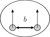
Figure 18: ${b}$ is the transverse interval between the quark and antiquark pair in the ${B}$ meson.

Then the Sudakov factor suppresses the long distance contributions for the decay process and gives the effective cutoff about the transverse direction Li:1992nu ; Collins:ta . In short, the Sudakov factor corresponds to the probability for emitting no photons. According to this factor, the property of short distance is guaranteed.

Figure 19: The dependence of the Sudakov factor ${\exp[-s(Q,b)]}$ on ${Q}$ and ${b}$ where ${Q}$ is the ${b}$ quark momentum, and ${b}$ is the interval between quarks which form hadrons. It is clear that the large ${b}$ and ${Q}$ region is suppressed.

Appendix B Some functions

The expressions for some functions are presented in this appendix. In our numerical calculation, we use the leading order ${\alpha_{s}}$ formula.

$$\alpha_{s}(\mu)=\frac{2\pi}{\beta_{0}\ln(\mu/\Lambda_{n_{f}})}_{,}\hskip 28.45274pt\beta_{0} = \frac{33-2n_{f}}{3}\hskip 8.53581pt$$ (112)

The explicit expression for Sudakov factor ${s(t,b)}$ is given by Botts:kf

$$s(t,b)=\int^{t}_{1/b}\frac{d\mu}{\mu}\left[\ln{\left(\frac{t}{\mu}\right)}A(\alpha_{s}(\mu))+B(\alpha_{s}(\mu))\right],$$ (113)

$$A = C_{F}\frac{\alpha_{s}}{\pi}+\left(\frac{\alpha_{s}}{\pi}\right)^{2}$$ (114)

$$\times\left[\frac{67}{9}-\frac{{\pi}^{2}}{3}-\frac{10}{27}n_{f}+\frac{2}{3}\beta_{0}\ln\left(\frac{e^{\gamma}_{E}}{2}\right)\right],$$

$$B = \frac{2}{3}\frac{\alpha_{s}}{\pi}\ln\left(\frac{e^{2\gamma_{E}}-1}{2}\right),$$ (115)

where ${\gamma_{E}=0.5722}$ is Euler constant and ${C_{F}=4/3}$ is color factor. The meson wave function including summation factor has energy dependence

$$\phi_{B}(x_{1},b_{1},t) = \phi_{B}(x_{1},b_{1})\exp{[-S_{B}(t)]},$$ (116)

$$\phi_{K^{*}}(x_{2},t) = \phi_{K^{*}}(x_{2})\exp{[-S_{K^{*}}(t)]},$$ (117)

and the total functions including the Sudakov factor and the ultraviolet divergences are

$$S_{B}(t) = s(x_{1}P_{1}^{-},b_{1})+2\int^{t}_{1/b_{1}}\frac{d\bar{\mu}}{\bar{\mu}}\gamma(\alpha_{s}(\bar{\mu})),$$ (118)

$$S_{K^{\ast}}(t) = s(x_{2}P_{2}^{-},b_{2})+s((1-x_{2})P_{2}^{-},b_{2})$$ (119)

$$\hskip 28.45274pt+2\int^{t}_{1/b_{2}}\frac{d\bar{\mu}}{\bar{\mu}}\gamma(\alpha_{s}(\bar{\mu})).$$

Threshold factor is expressed as below Li:2001ay ; Keum:2000wi , and we take the value ${c=0.4}$.

$$S_{t}(x)=\frac{2^{1+2c}\Gamma(3/2+c)}{\sqrt{\pi}\Gamma(1+c)}[x(1-x)]^{c}$$ (120)

Appendix C Wave functions

For the ${B}$ meson wave function, we adopt the model

$$\Phi_{B}(P_{1}) = \frac{1}{\sqrt{2N_{c}}}(\ooalign{\hfil/\hfil\crcr$P$}_{1}+M_{B})\gamma^{5}\phi_{B}(k_{1}),$$ (123)

$$\phi_{B}(x_{1},b_{1}) = \int dk_{1}^{-}d^{2}k_{1\perp}e^{i\vec{k}_{1\perp}\cdot\vec{b}}\phi_{B}(k_{1})$$ (124)

$$=N_{B}x_{1}^{2}(1-x_{1})^{2}\exp{\left[-\frac{1}{2}\left(\frac{x_{1}M_{B}}{\omega_{B}}\right)^{2}-\frac{b_{1}^{2}\omega_{B}^{2}}{2}\right]},$$

with th shape parameter ${\omega_{B}=(0.40\pm 0.04)}$GeV. The normalization constant ${N_{B}}$ is fixed by the decay constant ${f_{B}}$

$$\int^{1}_{0}dx\phi_{B}(x,b=0)=\frac{f_{B}}{2\sqrt{2N_{c}}}_{,}$$ (125)

where ${N_{c}}$ is the color number.

We use the vector meson wave functions determined by the light-cone QCD sum rule Ball:1998ff ; Ball:2003sc . We choose the vector meson momentum ${P}$ moving in the “-” direction along the ${z}$ axis with ${P^{2}=M_{V}^{2}}$, and the polarization vectors ${\epsilon_{L}}$, ${\epsilon_{T}}$ are defined as

$$\epsilon_{L}=(0,1,\vec{0}),\hskip 17.07164pt\epsilon_{T}=\left(0,0,\frac{1}{\sqrt{2}}(\pm 1,-i)\right),$$ (126)

and ${\epsilon_{T}}$ satisfies the gauge invariant condition ${P\cdot\epsilon_{T}=0}$. The nonlocal matrix elements sandwiched between the vacuum and the ${K^{*}}$ meson state can be expressed as follows,

$$\langle K^{\ast-}(P)\mid\bar{s}(z)Iu(0)\mid 0\rangle=\frac{1}{2N_{c}}f_{K^{\ast}}^{T}$$

$$\hskip 56.9055pt\times\frac{\epsilon_{L}\cdot z}{p\cdot z}M_{K^{\ast}}^{2}\int_{0}^{1}dxe^{ixP\cdot z}\frac{\partial}{\partial x}h_{\parallel}^{(s)}(x)$$

$$\langle K^{\ast-}(P)\mid\bar{s}(z)\gamma_{\mu}u(0)\mid 0\rangle=\frac{f_{K^{\ast}}}{N_{c}}M_{K^{\ast}}\Big{[}P_{\mu}\frac{\epsilon_{L}\cdot z}{P\cdot z}$$

$$\hskip 19.91692pt\times\int_{0}^{1}dxe^{ixP\cdot z}\phi_{\parallel}(x)+\epsilon_{T\mu}\int_{0}^{1}dxe^{ixP\cdot z}g_{\perp}^{(v)}(x)\Big{]}$$

$$\langle K^{\ast-}(P)\mid\bar{s}(z)\gamma_{5}\gamma_{\mu}u(0)\mid 0\rangle=-\frac{i}{4N_{c}}f_{K^{\ast}}$$

$$\hskip 14.22636pt\times\frac{M_{K^{\ast}}}{P\cdot z}\epsilon_{\mu\nu\rho\sigma}\hskip 2.84526pt\epsilon_{T}^{\nu}P^{\rho}z^{\sigma}\int_{0}^{1}dxe^{ixP\cdot z}\frac{\partial}{\partial x}g_{\perp}^{(a)}(x)$$

$$\langle K^{\ast-}(P)\mid\bar{s}(z)\sigma_{\mu\nu}u(0)\mid 0\rangle=-i\frac{f_{K^{\ast}}^{T}}{N_{c}}$$

$$\times\Big{[}(\epsilon_{T\mu}P_{\nu}-\epsilon_{T\nu}P_{\mu})\int_{0}^{1}dxe^{ixP\cdot z}\phi_{\perp}(x)$$

$$+(P_{\mu}z_{\nu}-P_{\nu}z_{\mu})\frac{\epsilon_{L}\cdot z}{(P\cdot z)^{2}}M_{K^{\ast}}^{2}\int_{0}^{1}dxe^{ixP\cdot z}h_{\parallel}^{(t)}(x)\Big{]}$$

where we neglect the terms proportional to ${r_{K^{*}}^{2}}$ (twist-4) and the terms ${(m_{u}+m_{s})/M_{K^{*}}}$. Then the ${K^{*}}$ meson distribution amplitudes up to twist-3 are

$$\Phi_{K^{*}}^{L}(P,\epsilon_{L}) = \frac{1}{\sqrt{2N_{c}}}\int_{0}^{1}dxe^{ixP\cdot z}\{M_{K^{\ast}}[\ooalign{\hfil/\hfil\crcr$\epsilon$}_{L}]\phi_{K^{\ast}}(x)$$ (138)

$$+[\ooalign{\hfil/\hfil\crcr$\epsilon$}_{L}\hskip 2.84526pt\ooalign{\hfil/\hfil\crcr$P$}]\phi_{K^{\ast}}^{t}(x)+M_{K^{\ast}}[I]\phi_{K^{\ast}}^{s}(x)\},$$

$$\Phi_{K^{*}}^{T}(P,\epsilon_{T}) = \frac{1}{\sqrt{2N_{c}}}\int_{0}^{1}dxe^{ixP\cdot z}\{M_{K^{\ast}}[\ooalign{\hfil/\hfil\crcr$\epsilon$}_{T}]\phi_{K^{\ast}}^{v}(x)$$ (147)

$$+[\ooalign{\hfil/\hfil\crcr$\epsilon$}_{T}\hskip 2.84526pt\ooalign{\hfil/\hfil\crcr$P$}]\phi_{K^{\ast}}^{T}(x)\hskip 2.84526pt+\frac{M_{K^{\ast}}}{P\cdot z}i\epsilon_{\mu\nu\rho\sigma}[\gamma^{\mu}\gamma^{5}]\epsilon_{T}^{\nu}P^{\rho}z^{\sigma}\phi_{K^{\ast}}^{a}(x)\}$$

$$\phi_{K^{\ast}}(x)=\frac{f_{K^{\ast}}}{2\sqrt{2N_{c}}}\phi_{\parallel},\hskip 8.53581pt\phi_{K^{\ast}}^{t}(x)=\frac{f_{K^{\ast}}^{T}}{2\sqrt{2N_{c}}}h_{\parallel}^{(t)},$$

$$\phi_{K^{\ast}}^{s}(x)=\frac{f_{K^{\ast}}^{T}}{4\sqrt{2N_{c}}}\frac{d}{dx}h_{\parallel}^{(s)},\hskip 8.53581pt\phi_{K^{\ast}}^{T}(x)=\frac{f_{K^{\ast}}^{T}}{2\sqrt{2N_{c}}}\phi_{\perp},$$

$$\phi_{K^{\ast}}^{v}(x)=\frac{f_{K^{\ast}}}{2\sqrt{2N_{c}}}g_{\perp}^{(v)},\hskip 8.53581pt\phi_{K^{\ast}}^{a}(x)=\frac{f_{K^{\ast}}}{8\sqrt{2N_{c}}}\frac{d}{dx}g_{\perp}^{(a)},$$

where we use ${\epsilon_{0123}=1}$ and set the normalization condition about ${\phi_{i}=\{\phi_{\parallel},\phi_{\perp},g_{\perp}^{(v)},g_{\perp}^{(a)},h_{\parallel}^{(t)},h_{\parallel}^{(s)}\}}$ as

$$\int_{0}^{1}dx\phi_{i}(x)=1.$$ (150)

${V}$	${K^{*}}$	${\rho}$
${f_{V}}$[MeV]	${226\pm 28}$	${198\pm 7}$
${f_{V}^{T}}$[MeV]	${185\pm 10}$	${160\pm 10}$
${a_{1}^{\parallel}}$[MeV]	${-0.4\pm 0.2}$	0
${a_{2}^{\parallel}}$[MeV]	${0.09\pm 0.05}$	${0.18\pm 0.10}$
${a_{1}^{\perp}}$[MeV]	${-0.34\pm 0.18}$	0
${a_{2}^{\perp}}$[MeV]	${0.13\pm 0.09}$	${0.2\pm 0.1}$
${\delta_{+}}$	0.24	0
${\delta_{-}}$	-0.24	0
${\tilde{\delta}_{+}}$	${0.16}$	0
${\tilde{\delta}_{-}}$	-0.16	0
${\zeta_{3}^{A}}$	0.032	0.032
${\zeta_{3}^{V}}$	0.013	0.013
${\zeta_{3}^{T}}$	0.024	0.024
${\omega_{1,0}^{A}}$	-2.1	-2.1

Table 4: Some parameter quantities.

$$\phi_{\parallel}(x) = 6x(1-x)\left[1+3a_{1}^{\parallel}x_{i}+\frac{3}{2}a_{2}^{\parallel}(5x_{i}^{2}-1)\right]$$

$$\phi_{\perp}(x) = 6x(1-x)\left[1+3a_{1}^{\perp}x_{i}+\frac{3}{2}a_{2}^{\perp}(5x_{i}^{2}-1)\right]$$

$$h_{\parallel}^{(s)}(x) = 6x(1-x)\left[1+a_{1}^{\perp}x_{i}+\left(\frac{1}{4}a_{2}^{\perp}+\frac{35}{6}\xi_{3}^{T}\right)(5x_{i}^{2}-1)\right]$$

$$+3\delta_{+}\left[3x(1-x)+x\ln x+(1-x)\ln(1-x)\right]$$

$$+3\delta_{-}\left[x\ln x-(1-x)\ln(1-x)\right]$$

$$h_{\parallel}^{(t)}(x) = 3x_{i}^{2}+\frac{3}{2}a_{1}^{\perp}x_{i}(3x_{i}^{2}-1)+\frac{3}{2}a_{2}^{\perp}x_{i}^{2}(5x_{i}^{2}-3)$$

$$+\frac{35}{4}\zeta_{3}^{T}(3-30x_{i}^{2}+35x_{i}^{4})+\frac{3}{2}\delta_{+}\left[1+x_{i}\ln\left(\frac{x}{1-x}\right)\right]$$

$$+\frac{3}{2}\delta_{-}{x_{i}}\left[2+\ln x+\ln(1-x)\right]$$

$$g_{\perp}^{(a)}(x) = 6x(1-x)\Big{[}1+a_{1}^{\parallel}\xi+\{\frac{1}{4}a_{2}^{\parallel}+\frac{5}{3}\zeta_{3}^{A}\left(1-\frac{3}{16}\omega_{1,0}^{A}\right)$$

$$+\frac{35}{4}\zeta_{3}^{V}\}(5x_{i}^{2}-1)\Big{]}+6\tilde{\delta}_{+}\Big{[}3x(1-x)+x\ln x$$

$$+(1-x)\ln(1-x)\Big{]}+6\tilde{\delta}_{-}\left[x\ln x-(1-x)\ln(1-x)\right]$$

$$g_{\perp}^{(v)}(x) = \frac{3}{4}(1+x_{i}^{2})+a_{1}^{\parallel}\frac{3}{2}x_{i}^{3}+\left(\frac{3}{7}a_{2}^{\parallel}+5\zeta_{3}^{A}\right)(3x_{i}^{2}-1)$$

$$+\left(\frac{9}{112}a_{2}^{\parallel}+\frac{105}{16}\xi_{3}^{V}-\frac{15}{64}\xi_{3}^{A}\omega_{1,0}^{A}\right)(3-30x_{i}^{2}+35x_{i}^{4})$$

$$+\frac{3}{2}\tilde{\delta}_{+}\left[2+\ln x+\ln(1-x)\right]$$

$$+\frac{3}{2}\tilde{\delta}_{-}\left[2x_{i}+\ln(1-x)-\ln x\right]$$

Here ${x_{i}=1-2x}$, and the expressions about ${\rho}$ and ${\omega}$ meson wave functions are the same as above with the values of parameters as follows evaluated at ${\mu=}$1GeV (Tab.4). Since ${\rho/\omega}$ states are ${(|\bar{u}u\rangle\mp|\bar{d}d\rangle)/\sqrt{2}}$, the ${\bar{q}q}$ distribution where ${q=u}$ or ${d}$ can be taken to the same for ${|\bar{u}u\rangle}$ and ${|\bar{d}d\rangle}$ using isospin symmetry.

References

- (1) S. Eidelman et al. [Particle Data Group], Phys. Lett. B 592 (2004) 1.
- (2) K. Abe et al. [BELLE Collaboration], arXiv:hep-ex/0409049.
- (3) B. Aubert et al. [BABAR Collaboration], arXiv:hep-ex/0408072.
- (4) M. Nakao et al. [BELLE Colaboration Collaboration], Phys. Rev. D 69, 112001 (2004) [arXiv:hep-ex/0402042].
- (5) B. Aubert et al. [BABAR Collaboration], Phys. Rev. D 70, 112006 (2004) [arXiv:hep-ex/0407003].
- (6) J. Alexander et al. [Heavy Flavor Averaging Group (HFAG) Collaboration], arXiv:hep-ex/0412073.
- (7) A. J. Buras, A. Czarnecki, M. Misiak and J. Urban, Nucl. Phys. B 631, 219 (2002) [arXiv:hep-ph/0203135].
- (8) G. Buchalla, A. J. Buras and M. E. Lautenbacher, Rev. Mod. Phys. 68, 1125 (1996) [arXiv:hep-ph/9512380].
- (9) M. Bauer and M. Wirbel, Z. Phys. C 42, 671 (1989).
- (10) Y. Y. Keum, H. n. Li and A. I. Sanda, Phys. Lett. B 504, 6 (2001) [arXiv:hep-ph/0004004].
- (11) P. Ball, V. M. Braun, Y. Koike and K. Tanaka, Nucl. Phys. B 529, 323 (1998) [arXiv:hep-ph/9802299].
- (12) P. Ball and M. Boglione, Phys. Rev. D 68, 094006 (2003) [arXiv:hep-ph/0307337].
- (13) M. Bander, D. Silverman and A. Soni, Phys. Rev. Lett. 43, 242 (1979).
- (14) J. Liu and Y. P. Yao, Phys. Rev. D 42, 1485 (1990).
- (15) H. Simma and D. Wyler, Nucl. Phys. B 344, 283 (1990).
- (16) H. n. Li and G. L. Lin, Phys. Rev. D 60, 054001 (1999) [arXiv:hep-ph/9812508].
- (17) E. Golowich and S. Pakvasa, Phys. Rev. D 51, 1215 (1995) [arXiv:hep-ph/9408370].
- (18) N. G. Deshpande, X. G. He and J. Trampetic, Phys. Lett. B 367, 362 (1996).
- (19) R. L. Anderson et al., Phys. Rev. Lett. 38, 263 (1977).
- (20) E. Paul, BONN-HE-81-26 Invited talk given at 10th Int. Symp. on Lepton and Photon Interactions at High Energy, Bonn, West Germany, Aug 24-29, 1981
- (21) K. Abe et al. [Belle Collaboration], Phys. Lett. B 538, 11 (2002) [arXiv:hep-ex/0205021].
- (22) B. Aubert et al. [BABAR Collaboration], Phys. Rev. Lett. 87, 241801 (2001) [arXiv:hep-ex/0107049].
- (23) M.Verderi, Workshop on the Unitarity Triangle in 2005, WG5 Session2, San Diego, 2005 (to be publushed)
- (24) A. L. Kagan, Phys. Lett. B 601, 151 (2004) [arXiv:hep-ph/0405134].
- (25) M. Beneke, T. Feldmann and D. Seidel, Nucl. Phys. B 612, 25 (2001) [arXiv:hep-ph/0106067].
- (26) A. Ali, E. Lunghi and A. Y. Parkhomenko, Phys. Lett. B 595, 323 (2004) [arXiv:hep-ph/0405075].
- (27) P. Ball and V. M. Braun, Phys. Rev. D 58, 094016 (1998) [arXiv:hep-ph/9805422].
- (28) L. Del Debbio, J. M. Flynn, L. Lellouch and J. Nieves [UKQCD Collaboration], Phys. Lett. B 416, 392 (1998) [arXiv:hep-lat/9708008].
- (29) D.Becirevic, talk presented at the Flavor Physics & CP Violation conference, Ecole Polytechnique, Paris France, June 2003
- (30) H. Y. Cheng and C. K. Chua, Phys. Rev. D 69, 094007 (2004) [arXiv:hep-ph/0401141].
- (31) A. Ali and A. Y. Parkhomenko, Eur. Phys. J. C 23, 89 (2002) [arXiv:hep-ph/0105302].
- (32) S. W. Bosch, arXiv:hep-ph/0208203.
- (33) S. W. Bosch and G. Buchalla, Nucl. Phys. B 621, 459 (2002) [arXiv:hep-ph/0106081].
- (34) C. H. Chen and C. Q. Geng, Nucl. Phys. B 636, 338 (2002) [arXiv:hep-ph/0203003].
- (35) A. L. Kagan and M. Neubert, Phys. Lett. B 539, 227 (2002) [arXiv:hep-ph/0110078].
- (36) M. Nagashima and H. n. Li, Phys. Rev. D 67, 034001 (2003) [arXiv:hep-ph/0210173].
- (37) H. n. Li and H. L. Yu, Phys. Rev. D 53, 2480 (1996) [arXiv:hep-ph/9411308].
- (38) J. C. Collins and D. E. Soper, Nucl. Phys. B 193, 381 (1981).
- (39) J. Botts and G. Sterman, Nucl. Phys. B 325, 62 (1989).
- (40) H. n. Li and G. Sterman, Nucl. Phys. B 381, 129 (1992).
- (41) H. n. Li, Phys. Rev. D 66, 094010 (2002) [arXiv:hep-ph/0102013].
- (42) T. Kurimoto, H. n. Li and A. I. Sanda, Phys. Rev. D 65, 014007 (2002) [arXiv:hep-ph/0105003].
- (43) J. C. Collins and G. Sterman, Nucl. Phys. B 185 (1981) 172.
-
(44)
Y. Y. Keum, H. N. Li and A. I. Sanda,
Phys. Rev. D 63 (2001) 054008
[arXiv:hep-ph/0004173].