Applications of instantons to hadronic processes

Abstract

Instantons constitute an important part of QCD as they provide a way to reach behind the perturbative region. In the introductory chapters we present, in the framework of a simple standard integral, the ideas that constitute the backbone of instanton computation. We explain why instantons are crucial for capturing non-perturbative aspects of any theory and get a feel for zero mode difficulties and moduli space. Within the same setting we explore the configuration space further by showing how constrained instantons and instanton valleys come into play.

We then turn our attention to QCD instantons and briefly show the steps to compute the effective lagrangian. We also show how single instanton approximation arises and how one can use it to evaluate correlation functions. By this we set the stage for the main parts of the thesis: computation of $\eta_{c}$ decay and evaluation of nucleon vector and axial vector couplings.

Having understood the effective lagrangian we use it as a main tool for studying instanton contributions to hadronic decays of the scalar glueball, the pseudoscalar charmonium state $\eta_{c}$, and the scalar charmonium state $\chi_{c}$. Hadronic decays of the $\eta_{c}$ are of particular interest. The three main decay channels are $K\bar{K}\pi$, $\eta\pi\pi$ and $\eta^{\prime}\pi\pi$, each with an unusually large branching ratio $\sim 5\%$. On the quark level, all three decays correspond to an instanton type vertex $(\bar{c}c)(\bar{s}s)(\bar{d}d)(\bar{u}u)$. We show that the total decay rate into three pseudoscalar mesons can be reproduced using an instanton size distribution consistent with phenomenology and lattice results. Instantons correctly reproduce the ratio $B(\pi\pi\eta)/B(\pi\pi\eta^{\prime})$ but over-predict the ratio $B(K\bar{K}\pi)/B(\pi\pi\eta(\eta^{\prime}))$. We consider the role of scalar resonances and suggest that the decay mechanism can be studied by measuring the angular distribution of decay products.

In the next part, motivated by measurements of the flavor singlet axial coupling constant of the nucleon in polarized deep inelastic scattering we study the contribution of instantons to OZI violation in the axial-vector channel. We consider, in particular, the $f_{1}-a_{1}$ meson splitting, the flavor singlet and triplet axial coupling of a constituent quark, and the axial coupling constant of the nucleon. We show that instantons provide a short distance contribution to OZI violating correlation functions which is repulsive in the $f_{1}$ meson channel and adds to the flavor singlet three-point function of a constituent quark. We also show that the sign of this contribution is determined by general arguments similar to the Weingarten inequalities. We compute long distance contributions using numerical simulations of the instanton liquid. We find that the iso-vector axial coupling constant of a constituent quark is $(g_{A}^{3})_{Q}=0.9$ and that of a nucleon is $g_{A}^{3}=1.28$, in good agreement with experiment. The flavor singlet coupling of quark is close to one, while that of a nucleon is suppressed $g_{A}^{0}=0.8$. This number is still significantly larger than the experimental value $g_{A}^{0}=(0.28-0.41)$.

Throughout the instanton computation in QCD one employs integration over the $SU(2)$ group as the $SU(2)$ parameters are part of the moduli space. The techniques of group integration are especially useful for computing the effective lagrangian. We therefore present an algorithm for computation of integrals over compact groups that is both simple and easy to implement. The main idea was mentioned before by Michael Creutz but, to our knowledge, never carried out completely. We exemplify it on integrals over $SU(N)$ of type $\int du(u{u}^{\dagger})^{n}$, with $n=1,2,3$ as well as integrals of adjoint representation matrices $\int du(R^{ab})^{n},n=1,\ldots 4$, $R^{ab}=\frac{1}{2}Tr(\lambda^{b}u\lambda^{a}u^{\dagger})$.

Chapter 1 Introduction

The physics of fundamental interactions is dominated today by the Standard Model(SM), the combined theory of strong, weak and electromagnetic force. Since its development in 1970’s it has proved extremely powerful in explaining the experimental results. The model has been so successful that, for thirty years, physicists have been desperately looking for a discrepancy between the model and experiment that would point them towards new physics ”beyond the standard model”.

Quantum chromodynamics(QCD), as a part of the Standard Model describes the gluon-mediated strong interactions between quarks. The origins of QCD date back to early 1960’s. The myriad of observed particles and their mass spectrum played then the same role as Mendeleev’s periodic table of elements a century ago: it pointed to the existence of underlying constituents, particles that represent a more elementary form of matter.

In 1964 Gell Mann and Zweig introduced spin-$\frac{1}{2}$ particles: up, down and strange quarks with fractional charge of $\frac{2}{3}$ for $u$ quark and $-\frac{1}{3}$ for $d$ and $s$ quarks. Assigning mesons to $\bar{q}q$ states and baryons to $qqq$ states using $SU(3)_{flavor}$ symmetry led to a good match of known particles and valuable predictions of new ones. (Valuable indeed, as Gell Mann was rewarded with Nobel Prize in 1969 for his ”Eightfold Way”).

However, the straight-forward quark model had to overcome the difficulty of reconciling the Pauli principle and the seemingly quark-exchange symmetric function of baryons made of 3 same-flavor quarks with the same spin, like $\Delta^{++}\sim u^{\uparrow}u^{\uparrow}u^{\uparrow}$. The solution came with an extra quantum number: color, that made it possible to antisymmetrize the baryonic state. Quarks would then come in three colors: red, green and blue and the hadrons would be composed of white combinations of quarks. Color-anticolor pairs of quark - antiquark would form mesons while baryons would be of type $\epsilon^{ijk}q_{i}q_{j}q_{k}$.

At this stage, the colored quarks were little more than mathematical objects that explained the spectrum of observed hadrons. The unsuccessful search for free spin-$\frac{1}{2}$ particles with fractional charge presented a big obstacle for the quark model to become more than a nice mathematical description of hadronic spectra. In late 1960’s, SLAC-MIT deep inelastic scattering experiments discovered point-like constituents, ”partons”, later identified with quarks. Eventually the discovery of $J/\Psi$ in 1974 in both hadroproduction and $e^{+}e^{-}$ annihilation finalized the conclusion that the quarks are real particles but are confined to colorless combinations.

The main conclusion of DIS experiments was the asymptotic freedom of proton constituents, which basically means that the interaction of partons is small for high energy transfer($\gtrsim 1\;{\rm GeV}$). This was an extra feature that any theory of strong interactions would need to possess.

QCD, the gauge theory of quarks based on $SU(3)$ group then emerged as the only viable candidate that would incorporate $N_{c}=3$ quarks, have a different representation for antiquarks and would feature asymptotic freedom and confinement.

On its way to maturity, QCD underwent a long series of experimental tests, like $\pi^{0}\to\gamma\gamma$ decay, deep inelastic scattering, $e^{+}e^{-}\to hadrons$ and so on. Most of the early successes were predominantly in the perturbative area of large momentum transfer and hence small coupling. In this sector, the methods of computation had already been known from QED and the Feynman diagrams techniques were readily available.

A completely different view was provided by lattice gauge theory methods, which use discretization of large but finite volume of spacetime and evaluate the path integral using Monte Carlo techniques. With increasing computational power the lattice QCD is becoming an accessible laboratory for non-perturbative physics. The main drawback of lattice QCD is the absence of analytic results from which one could get a better insight into the physical picture.

In the non-perturbative regime different analytic approaches have been developed that describe the physics at different energy scales. For small momenta well below 1 GeV the energetically accessible degrees of freedom are pions and other low-lying mesons. Therefore effective theories like the ones based on chiral lagrangians were natural tools successfully applied to physics of low energy pions. On the other side of particle spectrum, one can use the fact, that low energy interactions are less likely to create new heavy quark-antiquark pairs due to energy gaps. Therefore heavy quarkonia are accessible through non-relativistic quantum mechanical models similar to positronium treatment.

Instantons bridge the gap between the effective field theories and perturbative QCD. With their origins in the heart of QCD theory, they constitute one of the best understood non-perturbative tools. Instantons saturate the $U(1)_{A}$ anomaly and provide dynamical chiral symmetry braking. However, they do not solve the problem of confinement, which even after 30 years of work is still an open question.

The main tool for instanton computations is the instanton liquid model (ILM) developed in 1980’s. Is is based on the assumption that the vacuum is dominated by instantons. The parameters of the model, the mean density of instantons $n\cong 1\;{\rm fm^{-4}}$ and the average size of instantons $\rho\cong\frac{1}{3}\;{\rm fm}$ were fitted from the phenomenological values of quark and gluon condensates.

Among the successes of ILM are calculations of hadronic correlation functions, hadronic masses and coupling constants. A better understanding of chiral phase transition has also been achieved by studying instantons in finite temperature QCD.

In addition to that, we would like to identify direct instanton contributions to hadronic processes. One possibility is to go to very high energy, for example in DIS. In this case, instantons are very rare, but they lead to special processes with multi-gluon and quark emission, analogous to the baryon number violating instanton process in the electroweak sector.

In this work we focus on another possibility. The instanton induced interaction has very peculiar spin and flavor correlations that distinguish instantons from perturbative forces. We study two systems in which unusual flavor and spin effects have been observed: the decay of $\eta_{c}$ and the so-called ”proton spin crisis”.

First part of this work analysis the decay of $\eta_{c}$. The dominant decay channels have a specific structure of final products in which all pairs of constituent quarks are present. The resulting vertex is of type $(\bar{c}c)(\bar{s}s)(\bar{d}d)(\bar{u}u)$ which points to a possible instanton-induced mechanism behind the process.

The experimental evidence that quarks only carry about $30\%$ of the proton spin is contrary to the naive quark model predictions and it implies a large amount of OZI violation in the flavor singlet axial vector channel. The second part of this work studies the instanton contribution to this process.

1.1 High school instantons

1.1.1 Toy model instantons

Instanton is a finite-action solution of the euclidean equation of motion. Since it’s discovery in QCD in 1975 by Belavin et al [1] it has been enjoying considerable attention. In this section we will try to convey a feel for instanton physics without dipping into the details of any particular theory.

Many of the features of instanton computation can be easily explained on trivial examples that do not require more than high school integration. We will use the standard integral as an analog for the path integral. This way the ideas of the computation will be unveiled in full light without the technical difficulties blocking the view.

The single most important object in quantum field theory is the partition function, which can be represented as the path integral

$$Z[J]=\int\mathcal{D}\Phi e^{-S[\Phi,J]}$$

where $\Phi(x)$ is the field and $S[\Phi,J]$ is the action that also depends on the source $J$. Any correlation function can be computed once we know the partition function. Schematically:

$$<\Phi_{1}\Phi_{2}>=\delta_{J_{1}}\delta_{J_{2}}Z[J]$$

where $J_{1},J_{2}$ are the sources corresponding to $\Phi_{1},\Phi_{2}$.

It is usually not a trivial exercise to compute $Z[J]$. In fact, most of the time we are forced to rely on some kind of approximation. The standard technique is to expand the action around the trivial minimum ($\Phi\equiv 0$), keep the quadratic terms and treat the rest as a perturbation:

$$e^{-S[\Phi]}=e^{-S[0]-\frac{1}{2}\Phi S^{\prime\prime}[0]\Phi+O(\Phi^{3})}=e^{-\frac{1}{2}\Phi S^{\prime\prime}[0]\Phi}(1+O(\Phi^{3})+\cdots)$$ (1.1)

However, the perturbation approach usually does not, and can not, reach all the ’dark corners’ of the theory. The reason is the possible existence of other, non-trivial minima of the action, located in a different sector of the configuration space.

Figure 1.1: Action of a tilted double well potential.

To get a better feel about the approximations to the path integral, let us consider the most trivial toy-model for the path integral: QFT for a field in one point in spacetime. The configuration space is now considerably shrunk to one single variable, and the path integral is just a standard integral. As an example of theory with ’instanton’, let us take a tilted double well potential shown in Fig. 1.1:

$$S(\Phi)=\Phi^{2}(b^{2}(\Phi-a)^{2}+m).$$ (1.2)

The partition function is:

$$Z=\int_{-\infty}^{+\infty}d\Phi\>e^{-S(\Phi)}$$ (1.3)

Fig. 1.2 presents the graph of $e^{-S}$. The goal is to compute the area under the curve.

Figure 1.2: Exp(-S) for a tilted double well potential.

The approach corresponding to standard perturbation theory is to keep the quadratic terms in exponent and expand the rest:

$$e^{-S(\Phi)}=e^{-(m+a^{2}b^{2})\Phi^{2}}[1+O(\Phi^{3})+\cdots]$$ (1.4)

The graphs of zeroth and first order expansions are shown in Fig. 1.3. It is clear that in order to capture the full integral one needs a large order expansion. We can get a much better approximation of partition function by including the ’bump’ from the very beginning: just compute the additional area by repeating the perturbation approach for the smaller bump. Mathematically, its peak is at the minimum of the action, which is nothing else than the instanton. This separate term is the ’instanton’ contribution:

$$Z_{I}=\int d\Phi\>e^{-S(\Phi_{I})-\frac{1}{2}\left.\frac{d^{2}S}{d\Phi^{2}}\right|_{\Phi=\Phi_{I}}(\Phi-\Phi_{I})^{2}}(1+\cdots)$$ (1.5)

The total area under the curve would be the sum of the results of perturbation approach under both total and local minima of the action:

$$Z=Z_{0}+Z_{I}.$$

Figure 1.3: Zeroth (dashed line) and first (dotted line) order expansion around the trivial minima of the action are far away from giving a reasonable approximation to the $exp(-S)$. Bad news for perturbation theory: with higher order expansions, it gets worse before it gets better.

The zeroth order expansions under both minima are shown in Fig. 1.4. It is again obvious that this is a much better approximation of the integral than what we started with. A choice of $a=1$, $b=10$ and $m=0.4$ gives $Z_{0}=0.55$, $Z_{I}=0.43$ and $Z_{0}+Z_{I}=0.98$. The numerical integration gives $Z=0.99$.

Figure 1.4: The combined contribution of zeroth order expansions around both minima gives a clearly better approximation to the full integral.

In real models trivial fields and instantons live in separate, disconnected parts of configuration space. Therefore one not only needs to add instantons to get a better approximation with less computation, but has to account for instanton part in order to achieve the right result.

1.1.2 Zero modes and moduli space

There is a long shot from the trivial toy model to real world physics and many difficulties arise on the way. One of them, the zero modes and the moduli space is an omni-present feature that has to be dealt with in every instanton computation. The idea is easily explained on a ’next-to-trivial’ model of two spacetime points, i.e. a two-dimensional integral.

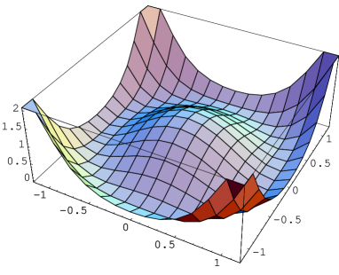
Figure 1.5: Sombrero action.

Let us consider the following ’sombrero’ action, depicted in Fig. 1.5, with the graph of $exp(-S)$ in Fig. 1.6:

$$S=(x^{2}+y^{2}-1)^{2}$$

As a result of the presence of rotational symmetry, we have a continuum of minima of action. The set of all ’instantons’ is a circle with radius 1. The parameters that describe it are called collective coordinates. In our case we can use an angle $\phi\in(0,2\pi)$:

$$(x,y)_{I}(\phi)=(\cos{\phi},\sin{\phi}).$$

The parameter space of all instantons is called the moduli space and in our case has the topology of a circle.

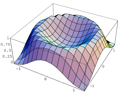
Figure 1.6: Exp(-S) for the sombrero action.

Suppose we did not have the err function available and decided to compute the integral numerically in a similar way we did it in the previous case of one-dimensional integral. We would need to expand around the minimum of the action. But which one should we choose? Let’s say we just pick an arbitrary minimum. The zeroth order expansion will now have a form of a two-dimensional distorted Gaussian bell, with different curvatures in different directions. If we press ahead and try to compute the volume under such a bell, we quickly run into difficulties: the result is infinite. Obviously this is not a problem of the integral, but of the method we used: the radius in one direction of the approximating two-dimensional Gaussian bell is infinity(the surface is flat in one direction corresponding to the symmetry direction). Therefore none of the minima alone is suited for an expansion.

This kind of difficulty appears every time we deal with a symmetry of the action that is broken by instanton. For each symmetry, there is an associated direction in the configuration space along which the action does not change. The vector that points in this direction is the zero mode. In our case it is the vector corresponding to a rotation, i.e. $\partial_{\phi}$, with $\phi$ being the azimuthal angle:

$$\vec{z}_{\phi}=\frac{d}{d\phi}\left(x,y\right)_{I}(\phi)=(-\sin{\phi},\cos{\phi})$$

The solution of the problem is obvious: one needs to turn the symmetry into an advantage, not a liability. The change of variables to polar coordinates is in order. To use the lingo of instanton physics, we will integrate over the direction of the zero mode non-perturbatively, leaving the perturbation method for the modes perpendicular to this. In other words, in one direction nothing changes, so we should just compute the one dimensional integral in the perpendicular direction and then multiply the result by the volume of the space in the zero mode direction.

Figure 1.7: At any point $(x^{\star},y^{\star})$ there is a zero mode direction and a ’perturbative’ direction. We integrate perturbatively along the ray while the integration over the azimuthal angle just gives the volume $2\pi$ of the moduli space.

Let us take as a starting point of our integration an arbitrary point $(x^{\star},y^{\star})\neq(0,0)$. The one-dimensional space perpendicular to the zero mode in this point is the line $(x,y)\cdot\vec{z}_{\phi}\equiv-x\sin{\phi}+y\cos{\phi}=0$ with $\tan{\phi}=\frac{y^{\star}}{x^{\star}}$ - see Fig 1.7. For every point on the line, we only want to integrate radially, and leave the perpendicular direction for later. This can be achieved by introducing the following delta function in the integral:

$$\delta((x,y)\cdot\vec{z}_{\phi})=\delta(-x\sin{\phi}+y\cos{\phi})$$

which forces the integration points lay on the line. To obtain the contribution over the whole plane we only need to integrate over the angle, with a weight that makes the whole insertion a unity :

$$\Delta(x,y)\int_{0}^{2\pi}\delta(-x\sin{\phi}+y\cos{\phi})d\phi=1$$

It is easy to compute $\Delta(x,y)=\frac{1}{2}\sqrt{x^{2}+y^{2}}$. The whole integral then is:

$$\int\!dxdy\;e^{-S(x,y)}\frac{1}{2}\sqrt{x^{2}+y^{2}}\int_{0}^{2\pi}\delta(-x\sin{\phi}+y\cos{\phi})d\phi$$

After a change of variables

$$x^{\prime} = x\cos{\phi}-y\sin{\phi}$$

$$y^{\prime} = -x\sin{\phi}+y\cos{\phi}$$

and evaluation of integral over $y^{\prime}$ one obtains

$$\int_{0}^{2\pi}\!\delta\phi\times\frac{1}{2}\int_{-\infty}^{+\infty}\!dx^{\prime}\;e^{-S(x^{\prime},0)}\sqrt{x^{\prime 2}}$$ (1.6)

The result is nothing else but the volume of moduli space multiplied by the integral in radial direction(integral over non-zero modes). Now we could expand the radial integral around the 2 bumps it contains in the very same way we did it in the example from the beginning of this section.

The main step in dealing with zero modes is their separation from ’perturbative’ direction by requiring the scalar product to be zero:

$$(x,y)\cdot\vec{z}_{\phi}=0$$ (1.7)

Another interesting interpretation is the following. The question is around which of the continuum of instantons one should expand. A very intuitive approach would be to expand different parts of space around different instanton, mainly, the $closest$ one. Let us take again the starting point $(x^{\star},y^{\star})$. The closest instanton is given by the minimization of the distance

$$min_{\phi}||(x^{\star},y^{\star})-(\cos{\phi},\sin{\phi}||^{2}$$

A differentiation w.r.t. $\phi$ gives the same condition 1.7. One would then separate the configuration space into blocks, each one of them being dominated by the closest instanton. In our case a block would be a ray with angle $\phi$ and the points on the ray would be under the ’jurisdiction’ of the instanton at $(\cos{\phi},\sin{\phi})$. Adding the contributions of all rays would lead to the same result 1.6.

1.1.3 Valley instantons and all that

We should be on a pretty good footing now that we know how to deal with a continuum of minima. For any integral we would find all minima and expand around them, paying special attention to treatment of zero modes. This kind of ’turning the crank’ could actually lead to a poor result in some cases, when there are a lot of important points without satisfying the condition of minimum.

The presence of an ’almost zero mode’, a direction with very low gradient, would make the Gaussian bell around the minima a poor approximation of the integral. To get a better understanding, let us take again the sombrero action and slightly tilt it:

$$S=(x^{2}+y^{2}-1)^{2}-\epsilon x$$

The graph of the tilted sombrero action with $\epsilon=\frac{1}{2}$ is shown in Fig. 1.8. The surface now exhibits a single global minimum - the instanton - close to the point $(1,0)$ and a saddle point close to $(-1,0)$. The exponent of tilted action is shown in Fig. 1.9.

If $\epsilon$ is small, the volume under the surface of $e^{-S}$ of the tilted sombrero will not differ significantly from the original one. In fact, one could obtain an $\epsilon$-expansion of the integral. However, our method of expanding around minima would fail, as the single Gaussian bell centered at the global minimum of $S$ would not describe well the whole surface.

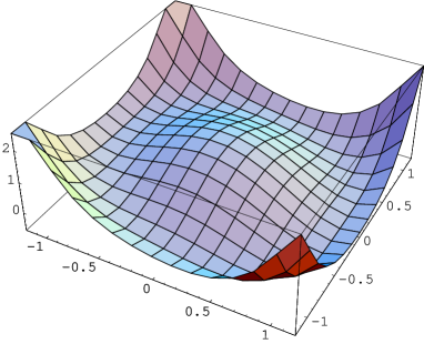
Figure 1.8: Tilted sombrero action.

Since $\epsilon$ is small, we should, in principle do something similar to $\epsilon=0$ case discussed in the previous section. For that reason, we first need to identify the important points - ’valley instantons’ - that are dominant, in some way, for ${\rm exp}(-S)$ in their restricted vicinity. Let us postpone for a moment the strict definition of the valley points. Intuitively it is clear, that in our case, the special points would form a loop $\epsilon$-close to the former circle of instantons. Once we have the valley trajectory, we would integrate perturbatively in the sector perpendicular to valley in the same way we treated the non-zero modes before. Now the final integral along the valley trajectory would not simply give the volume of the would-be moduli space, as the result of integration over non-valley directions depends on the parameter of the given point on trajectory.

We still have not defined precisely the valley trajectory. There are actually two approaches with slightly different results: the streamline [3, 4] and the so-called proper valley [5] method.

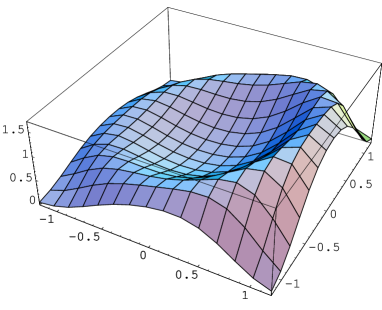
Figure 1.9: exp(-S) for tilted sombrero action.

The streamline method requires a starting point located on the trajectory but different from the global minimum. In our case it could be the saddle point. Having the starting point, the instanton valley is constructed dynamically by following the highest slope downwards. It is exactly the path a stream of water would follow - hence the name.

The proper valley method features more stability and does not require any starting point. The valley is now made of points with the lowest gradient along the contour of equal action. One should therefore draw the contour lines (’izoactas’) and for each of them identify the point with lowest gradient. Joining these points would give the trajectory.

Once we have the trajectory, we can start turning the crank again: at each point of the valley integrate perturbatively over modes perpendicular to the trajectory and then integrate over the trajectory of the valley.

Another approach to the same problem uses so-called ’constrained instantons’ [6, 7]. The idea is very simple: slice the configuration space in surfaces given by a family of functions. In our case one could take the slices generated by the family of vertical planes $x=\alpha$, with $\alpha\in(-\infty,+\infty)$. For example, the slice generated by $x=0$ is just the standard double well potential in $y$ direction. Each slice would feature constrained minima which one could use to compute the integral over the slice. At the end, one would only need to sum over the slices, i.e. integrate over $\alpha$.

The ambiguity of choosing the slicing function makes this approach less appealing. One has to have some physical intuition to use it with success. In our case, the almost-symmetry of the graph would point to slicing by rays $-x\sin{\phi}+y\cos{\phi}=0$.

There is a lot one can learn about the methods of path integration from a standard 2 dimensional high-school integral. We will now take the earned intuition and apply it to instantons in QCD.

1.2 Instantons in QCD

In this section we will focus on providing the main ideas for the derivation of the effective Lagrangian as well as on setting the stage for using the single instanton approximation for computing correlation functions. A thorough review on instantons in QCD can be found in [24].

As mentioned before, instantons are finite action solutions of equation of motion in Euclidean spacetime. For a Yang-Mills theory, the partition function reads:

$$Z=\mathbf{\int\!\!\mathcal{D}A}e^{-S_{YM}}$$

where

$$S_{YM}=\frac{1}{4g^{2}}\int d^{4}xF^{a}_{\mu\nu}F^{a}_{\mu\nu}$$

and $F_{\mu\nu}=\partial_{\mu}A_{\nu}-\partial_{\nu}A_{\mu}+[A_{\mu},A_{\nu}]$ is the field strength. Let us for simplicity consider $SU(2)$ YM theory. The requirement of a finite action leads to fields that tend to pure gauge at infinity: $A_{\mu}\to u^{-1}\partial_{\mu}u$, with $u\in SU(2)$. The infinity is topologically a 3-sphere. The instanton at infinity is therefore a map from the spatial $S^{3}$ to $S^{3}$ of $SU(2)$ parameters. Every such a mapping is characterized by a winding number, an integer that shows how many times one sphere is wrapped around the other by the map.

Figure 1.10: The instanton at infinity is a mapping from spatial 3-sphere to 3-sphere of $SU(2)$ parameters. Each such mapping is characterized by integer winding number.

The whole configuration space of finite-action gauge fields is then separated into distinct sectors characterized by different values of winding number. Figs. 1.11 and 1.12 show schematically the action $S$ and $e^{-S}$ in the sectors of $n=0$ (zero winding number), $n=1$ (one instanton) and $n=2$ (two instantons). The sectors are completely separated by infinite action walls, in the sense that any trajectory from one sector to another will have points where $S_{YM}=\infty$. It is exactly because of this separation that one has to account for instanton contributions, as one can not retrieve them from $n=0$ sector.

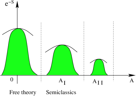
Figure 1.11: Schematic representation of quadratic approximation in different sectors of the configuration space.

Before plunging into any instanton computation, one has to deal first with gauge invariance. As any other symmetry, it induces zero modes and flat directions, derailing the perturbative approach. The way around this difficulty was explained on the toy model of section 1.1: integrate over zero modes direction non-perturbatively, then compute quantum fluctuations perpendicular to zero modes. In the case of gauge invariance, this means fixing the space for quantum fields by requiring

$$\mathbf{D}_{\mu}^{I}A_{\mu}^{qu}=0$$

where $\mathbf{D}_{\mu}^{I}$ is the covariant derivative in a background field. After exponentiating the Fadeev-Popov determinant, the action becomes a functional of ghost fields $b$ and $c$:

$$Z=\mathbf{\int\!\!\mathcal{D}A}\mathbf{\mathcal{D}b}\mathbf{\mathcal{D}c}\>e^{-\mathcal{S}[A,b,c]}$$

$$\mathcal{S}=\int d^{4}x\left\{\frac{1}{4g^{2}}F^{a}_{\mu\nu}F^{a}_{\mu\nu}+\frac{1}{2}(\mathbf{D}_{\mu}^{I}A_{\mu}^{a})^{2}+\mathbf{D}_{\mu}^{I}b^{a}\mathbf{D}_{\mu}^{I}c^{a}\right\}$$

1.2.1 Effective Lagrangian for gauge fields

The instanton solution of the equation of motion reads:

$$A_{\mu}^{(cl)} = 2\rho^{2}\frac{\bar{\eta}_{\mu\nu}^{a}(x-x_{0})_{\nu}}{(x-x_{0})^{2}((x-x_{0})^{2}+\rho^{2})}u\frac{\tau^{a}}{2}\bar{u}$$

$$b^{a} = c^{a}=0$$ (1.8)

where $A_{\mu}^{(cl)}$ is the instanton configuration with the center at $x_{0}^{\mu}$ and orientation given by the $SU(2)$ matrix $u$. Here $\tau^{a}$ is the Pauli matrix and $\bar{\eta}^{a}_{\mu\nu}$ is the t’Hooft tensor with properties given e.g. in [24].

Let us now explore the semiclassical approach, i.e. perturbation theory around the minima of the action. Expanding the action in the functional Taylor series and keeping the terms up to second order we obtain, for the gauge sector:

$$e^{-\mathcal{S}}=e^{-\mathcal{S}[A^{(cl)}]-\frac{1}{2}AM_{A}A+...}$$

Even after fixing the gauge, we are still left with a rigid gauge symmetry that brings $4N-5$ zero modes, where $N$ is the number of colors. Besides that, there are 5 flat directions corresponding to scaling and translational invariance. The remaining $SO(4)$ rotational symmetry does not bring any new zero modes, as any such rotation can be undone by a gauge rotation. In other words, the $SO(4)$ rotational zero mode points to the space unavailable to quantum fluctuations, as they were made perpendicular to gauge zero modes by fixing the gauge. Therefore altogether there are $4N$zero modes.

Figure 1.12: YM action in different winding number sectors

The non-perturbative integration over the zero mode directions and subsequent computation of quantum fluctuations limited to Gaussian approximation gives

$$\frac{Z}{Z_{0}}=\int\prod_{i=1}^{4N}\frac{d\gamma^{i}}{\sqrt{2\pi}}\left[2^{4}\rho^{2(4N-5)}\mathcal{S}_{cl}^{4N}\right]^{\frac{1}{2}}e^{-\mathcal{S}_{cl}}\times$$

$$\times\left(\frac{\det^{\prime}M_{A}}{\det M_{A}^{0}}\right)^{-1/2}_{reg}\left(\frac{\det^{\prime}M_{gh}}{\det M_{gh}^{0}}\right)_{reg},$$

where prime on determinants means that zero eigenvalues are not included. The computation of determinants was performed in [2] and the full result is:

$$\frac{Z}{Z_{0}}=C\int d^{4}x_{0}\frac{d\rho}{\rho^{5}}\int d\Omega\frac{1}{g^{4N}}e^{-\frac{8\pi^{2}}{g^{2}(\rho)}}\equiv\int d\mu_{I}$$

For completeness, the constant is

$$C=\frac{2^{4N+2}\pi^{4N-2}}{(N-1)!(N-2)!}\>e^{-\alpha(1)-2(N-2)\alpha(\frac{1}{2})}$$

with $\alpha(1)=0.443$ and $\alpha(\frac{1}{2})=0.145$

Let us now push the computation one step further and obtain the instanton-induced effective Lagrangian. We are interested in computing the correlations of the type:

$$<A_{\mu}^{a}(x)A_{\nu}^{b}(y)>_{I}=\frac{1}{Z}\mathbf{\int\!\!\mathcal{D}A}\mathbf{\mathcal{D}b}\mathbf{\mathcal{D}c}\>e^{-\mathcal{S}[A,b,c]}A_{\mu}^{a}(x)A_{\nu}^{b}(y)$$

Expanding near instanton $A_{\mu}=A_{\mu}^{(cl)}+A_{\mu}^{(qu)}$ we obtain:

$$<A_{\mu}^{a}(x)A_{\nu}^{b}(y)>_{I}=\int\!\!d\mu_{I}A_{\mu}^{a,(cl)}(x)A_{\nu}^{b,(cl)}(y)+<A_{\mu}^{a,(qu)}(x)A_{\nu}^{b,(qu)}(y)>$$

Instead of computing the correlations this way, we are interested in an effective potential $\mathbf{V}_{I}$ such that for large distance, $|x-x_{0}|^{2}>>\rho^{2}$, one retrieves the instanton fields:

$$<A_{\mu}^{a}(x)A_{\nu}^{b}(y)>_{I}=<A_{\mu}^{a}(x)A_{\nu}^{b}(y)\mathbf{V}_{I}>_{pert}$$

One can check, that Callan Dashen and Gross (CDG) potential [26]:

$$\mathbf{V}_{I}\equiv V_{CDG}=\int\!\!d\mu_{I}\exp{\left[-\frac{\pi^{2}\rho^{2}}{g^{2}}\eta_{\mu\nu}^{b}\>Tr[\tau^{b}\bar{u}\tau^{a}u]F^{a}_{\mu\nu}\right]}$$

provides exactly this. To see that this is indeed the case, let us compute the gauge field propagator in the instanton background for large distance. The second order expansion in $\eta F$ gives, schematically:

$$<A_{\mu}(x)A_{\nu}(y)\mathbf{V}_{I}>=\int\!\!d\mu_{I}<A_{\mu}(x)A_{\nu}(y)\eta F\eta F>$$

Disregarding the vacuum bubbles and next order corrections in the coupling constant, one is left with terms like

$$<A_{\mu}^{a}(x)F^{b}_{\alpha\beta}(x_{0})>=\frac{2g^{2}}{(2\pi)^{2}}\delta^{ab}\frac{[\delta_{\mu\beta}(x-x_{0})_{\alpha}-\delta_{\mu\alpha}(x-x_{0})_{\beta}]}{(x-x_{0})^{4}}$$

This way every $A_{\mu}(x)$ field will contribute a factor of

$$2\rho^{2}\frac{\eta_{\mu\nu}^{a}(x-x_{0})_{\nu}}{(x-x_{0})^{4}}u\frac{\tau^{a}}{2}\bar{u}$$

which is just the large distance limit of instanton field.

The anti-instanton fields lead to similar expressions with the substitutions $u\leftrightarrow\bar{u}$ , $\eta\leftrightarrow\bar{\eta}$.

1.2.2 Fermions and t’Hooft vertex

We will introduce now the fermionic degrees of freedom and study how this affects the computation in the instanton background.

t’Hooft’s discovery of left-handed zero mode of the Dirac operator in the presence of instanton came a little bit as a surprise with huge implications. First of all the zero mode renders the tunneling amplitude zero in case of massless quarks, as the tunneling is proportional to the determinant of Dirac operator. However, the instanton contribution to some Green’s functions is non-zero and clearly distinguishable from the perturbative contribution. In these correlations the small mass parameter $m$ from the Dirac determinant cancels against $\frac{1}{m}$ from the zero mode propagator, as we will show below.

The specific helicity of zero mode also pointed to chiral symmetry braking, and in fact solved the $\eta^{\prime}$ puzzle.

Let us now dip into some details of t’Hooft’s computation. The fermionic part of QCD action reads:

$$\mathcal{S}[\psi,J]=\!\!\int dx\>\bar{\psi}(x)(/\!\!\!\!D+m)\psi(x)-\int\!\!\!\!\int dx\>dy\>\>\bar{\psi}_{s}(x)J_{st}(x,y)\psi_{t}(y)$$

where $J_{st}$ is the source used to generate bilinear fermionic fields.

The massless Dirac operator in the instanton background has a left-handed zero mode:

$$\psi^{0}(x)=\frac{\rho}{\pi}\frac{1}{(x^{2}+\rho^{2})^{3/2}}\frac{/\!\!\!x}{\sqrt{x^{2}}}\frac{1+\gamma_{5}}{2}\Phi$$

with $\Phi^{\alpha m}=\frac{\epsilon^{\alpha m}}{\sqrt{2}}$. The semiclassical result will now have an extra determinant:

$$\frac{Z}{Z_{0}}=\!\int\!\!d\mu_{I}\rho^{N_{f}}m^{N_{f}}e^{[-\frac{2}{3}N_{f}\ln(\mu_{0})\rho+2N_{f}\alpha(1/2)]}\equiv\int\!\!d\mu_{I,f}$$

This shows that the tunneling is suppressed in the presence of light fermions by a factor of $m^{N_{f}}$.

To compute the Green’s functions we differentiate with respect to the source:

$$<\bar{\psi}^{s}_{\alpha}(x)\psi^{t}_{\beta}(y)>=\left.\frac{\delta}{\delta J^{st}_{\alpha\beta}(x,y)}\frac{Z[J]}{Z[0]}\right|_{J=0}.$$

$Z[J]$ depends on $J$ through $\det M_{\psi}$:

$$\det M_{\psi}=\det(-/\!\!\!\!D\delta_{st}+J_{st}).$$

Let us take for simplicity the propagator for one flavor. Then the determinant of Dirac operator with the source is given in terms of the eigenvalues $\lambda_{n}^{J}$:

$$\det M_{\psi}=\prod_{n}\lambda_{n}^{J},$$

where $\lambda_{n}^{J}$ satisfy $(-/\!\!\!\!D+J)\psi=\lambda_{n}^{J}\psi$. Expanding $\lambda_{n}^{J}$ in powers of J we get:

$$\lambda_{n}^{J}=\lambda_{n}^{J=0}+\alpha_{n}\cdot J+\ldots$$

where $\alpha_{n}\cdot J=\int\!\!\int dx\>dy\>\>\alpha_{n}(x,y)\>J(x,y)$. The propagator then involves:

$$\delta_{J_{\alpha\beta}}\left.\prod_{n}(\lambda_{n}^{J=0}+\alpha_{n}\cdot J)\right|_{J=0}=\left.\delta_{J_{\alpha\beta}}\left[(\alpha_{0}\cdot J)(\lambda_{1}+\alpha_{1}\cdot J)\ldots\right]\right|_{J=0}\;.$$

The final evaluation at $J=0$ renders all but one term zero. After simplification with $Z[0]$ we obtain

$$<\bar{\psi}_{\alpha}\psi_{\beta}>=\frac{1}{m}\alpha_{0{\beta\alpha}}\;,$$

which is nothing else but the first correction to zero energy due to source, i.e. standard perturbation theory

$$(\alpha_{0}\cdot J)=<\psi^{0}|J|\psi^{0}>\;.$$

Then the zero mode part of the propagator reads:

$$<\bar{\psi}_{\alpha}(x)\psi_{\beta}(y)>=\frac{1}{m}{\psi^{0}}^{*}_{\alpha}(x)\psi^{0}_{\beta}(y)\;.$$

Note the $\frac{1}{m}$ factor that will cancel with $m$ from the Dirac determinant to give finite correlation functions.

In the case of many massless quarks, the operator $(-/\!\!\!\!D\delta_{st}+J_{st})$ has $N_{f}$ times degenerate ground state. The surviving term in a Green’s function is then the product of perturbed eigenvalues, which can be written as the determinant of ’perturbation matrix’:

$$\prod_{i=1}^{N_{f}}(\alpha_{0}^{i}\cdot J)=det_{st}<\psi^{0}|J_{st}|\psi^{0}>=det_{st}\int\!\!dxdy\;{\psi^{0}}^{*}(x)J_{st}(x,y)\psi^{0}(y)\;.$$

This clearly points to the following properties of the Green’s functions in the zero mode approximation of the instanton computation:

• at least $2N_{f}$ fermions participate (otherwise the contribution is of the higher order than zero modes).

• It has a determinantal structure in flavor, all flavors must be there in pairs

• Quarks propagate in the left-handed mode, while anti-quarks in the right-handed mode.

• One can not have 2 fermions propagating in the same zero mode( this is the instantonic version of Pauli principle)

The graphical representation of the instanton vertex is shown in the Fig. 1.13.

Figure 1.13: Instanton vertex contains all the pairs of light quarks. Particles are left-handed while anti-particles are right handed.

Let us now construct the fermionic effective lagrangian. The idea is the same as for the gauge field effective vertex: we need to find $L_{t^{\prime}H}$ such that:

$$<\bar{\psi}_{\alpha}(x)\psi_{\beta}(y)L_{t^{\prime}H}>_{pert}=\langle\bar{\psi}\psi\rangle_{inst}=\frac{1}{m}{\psi}^{*}_{\alpha}(x)\psi_{\beta}(y)$$

$$=\frac{\rho^{2}}{m\pi^{2}}\frac{\left((/\!\!\!x-/\!\!\!x_{0})\frac{1+\gamma_{5}}{2}\Phi\right)^{+}_{\alpha}}{(x-x_{0})^{4}}\frac{\left((/\!\!\!y-/\!\!\!x_{0})\frac{1+\gamma_{5}}{2}\Phi\right)_{\beta}}{(y-x_{0})^{4}}$$ (1.9)

t’Hooft proposed a Lagrangian of the type:

$$S_{t^{\prime}H}=\int\!\!d\mu_{I,f}K(\bar{\psi}\omega)(\bar{\omega}\psi)$$

with K a constant and $\omega$ a spinor to be determined. First order expansion of the exponent of action gives for fermion propagator:

$$<\bar{\psi}_{\alpha}(x)\psi_{\beta}(y)(\bar{\psi}\omega)(\bar{\omega}\psi)>=\left(\frac{/\!\!\!y-/\!\!\!x_{0}}{2\pi^{2}(z-x_{0})^{4}}\right)_{\beta\gamma}\omega_{\gamma}\bar{\omega}_{\delta}\left(\frac{/\!\!\!x-/\!\!\!x_{0}}{2\pi^{2}(x-x_{0})^{4}}\right)_{\delta\alpha}$$

which leads to the r.h.s. of 1.9 if we choose $\omega=\frac{1+\gamma_{5}}{2}\Phi$ , $K=4\rho^{2}\pi^{2}/m$

To make it gauge symmetric we average over all possible orientations of $\omega$ to get:

$$S_{t^{\prime}H}=\int d\mu_{I,f}\left(4\pi^{2}\rho^{3}\bar{\psi}^{a}(x_{0})\left(\frac{1+\gamma_{5}}{2}\right)\psi^{a}(x_{0})\right)$$

Combining the many-flavors fermionic and gluonic effective lagrangians, the large-distance effects of instantons can be represented by the following lagrangian [26, 27, 28, 29]:

$${\cal L}_{I} = \int\prod_{q}\left[m_{q}\rho-2\pi^{2}\rho^{3}\bar{q}_{R}\left(U\mathbf{1}_{2}U^{\dagger}+\frac{i}{2}t^{a}R^{aa^{\prime}}\bar{\eta}^{a^{\prime}}_{\mu\nu}\sigma^{\mu\nu}\right)q_{L}\right]$$ (1.10)

$$\times\exp\left(-\frac{2\pi^{2}}{g}\rho^{2}\bar{\eta}^{b^{\prime}}_{\gamma\delta}R^{b^{\prime}b}G^{b,\gamma\delta}\right)dz\frac{d_{0}(\rho)}{\rho^{5}}d\rho\;dU.$$

where $t^{a}=\frac{1}{2}\lambda^{a}$ with ${\rm tr}[\lambda^{a}\lambda^{b}]=2\delta^{ab}$ are $SU(3)$ generators, ${1}_{2}={\rm diag}(1,1,0)$, $\eta^{a}_{\mu\nu}$ is the ’t Hooft symbol and $\sigma_{\mu\nu}=\frac{1}{2}[\gamma_{\mu},\gamma_{\nu}]$. The instanton is characterized by $4N_{c}$ collective coordinates, the instanton position $z$, the instanton size $\rho$, and the color orientation $U\in SU(N_{c})$. We also define the rotation matrix $R^{ab}$ by $R^{aa^{\prime}}\lambda^{a^{\prime}}=U\lambda^{a}U^{\dagger}$. For an anti-instanton we have to replace $L\leftrightarrow R$ and $\bar{\eta}\leftrightarrow\eta$. The semi-classical instanton density $d(\rho)$ is given by

$$d(\rho)=\frac{d_{0}(\rho)}{\rho^{5}}=\frac{0.466\exp(-1.679N_{c})1.34^{N_{f}}}{(N_{c}-1)!(N_{c}-2)!}\,\left(\frac{8\pi^{2}}{g^{2}}\right)^{2N_{c}}\rho^{-5}\exp\left[-\frac{8\pi^{2}}{g(\rho)^{2}}\right],$$ (1.11)

where $g(\rho)$ is the running coupling constant. For small $\rho$ we have $d(\rho)\sim\rho^{b-5}$ where $b=(11N_{c})/3-(2N_{f})/3$ is the first coefficient of the beta function.

The need for this lagrangian is not obvious from computations of correlation functions, as one can do well without it(better actually), since direct use of instanton solution and fermionic zero mode is correct at any distance. However, the effective lagrangian becomes a great tool if one tries to compute the instanton contribution to matrix elements of type $<\eta_{c}|K\bar{K}\pi>$. Our inability to write pion fields in terms of more fundamental quark creation/annihilation operators renders the straight-forward approach of computing correlation functions inapplicable. As we shall see in chapter 2, there are still ways to employ the effective lagrangian and compute the matrix element as

$$<\eta_{c}|K\bar{K}\pi>_{inst}=<\eta_{c}|\int\!\!d\mu_{I,f}V_{t^{\prime}H}V^{CDG}|K\bar{K}\pi>.$$

Another great advantage of the effective lagrangian is that it displays transparently the physical properties of the interaction. This way one easily gains physical intuition by thinking in terms of Feynman diagrams.

1.2.3 Dilute gas approximation

The instanton is a theoretically tractable non-perturbative object. However, the QCD vacuum proved to be much more complicated. A good description has been achieved by constructing the vacuum from instantons and anti-instantons. Within this framework, dilute gas approximation leads to a manageable computation, where multiple instanton effects can be computed from single instanton. In this section, following [72], [73] we will present the main ideas of dilute gas and single instanton approximation.

Configuration space of finite-action gauge fields consists of disjunct subspaces characterized by different winding numbers. The vacuum expectation value of an operator $\Pi$ is given as the sum over these sectors of different homotopy number n:

$$\langle vac|\Pi|vac\rangle=\frac{\sum_{n=-\infty}^{+\infty}\int\left[DA_{\mu}D\psi D\bar{\psi}\right]_{n}e^{-S(A,\psi,\bar{\psi})}\Pi(A,\psi,\bar{\psi})}{\sum_{n=-\infty}^{+\infty}\int\left[DA_{\mu}D\psi D\bar{\psi}\right]_{n}e^{-S(A,\psi,\bar{\psi})}}$$ (1.12)

Semiclassical approximation amounts to getting the minimum of action in each sector (solution of the equations of motion) and performing the Gaussian approximation around this solution. In each sector, a multi-instanton configuration is the true minimum of the action. However, it has been argued that the superposition of well separated $n_{+}$ instantons and $n_{-}$ anti-instantons, such that $n_{+}-n_{-}=n$ has a much higher entropy then the true minima for the sector with winding number $n$, therefore dominating the path integral. . The expansion around these approximate solutions provide a very good description of the true vacuum of QCD. Moreover, the Gaussian approximation proves to be expressible through the measure of a single instanton, in case one neglects the interaction between the instantons. Neglecting other minima, the path integral (1.12) can therefore be written as a dilute gas:

$$\langle vac|\Pi|vac\rangle=\frac{\sum_{n_{+},n_{-}}\frac{1}{n_{+}!n_{-}!}\int(d\mu_{+})^{n_{+}}(d\mu_{-})^{n_{-}}\langle\Pi\rangle_{A_{n_{+},n_{-}}}}{\sum_{n_{+},n_{-}}\frac{1}{n_{+}!n_{-}!}\int(d\mu_{+})^{n_{+}}(d\mu_{-})^{n_{-}}}$$ (1.13)

where $d\mu_{\pm}$ is instanton measure of moduli space. Phenomenological estimates give the density of instantons to be of the order of $n\approx 1\;{\rm fm}^{-4}$ while the mean instanton size has been found to be $\bar{\rho}\approx 0.3\;{\rm fm}$. The dimensionless parameter $\bar{\rho}^{4}n\cong 0.008$ shows that the instanton liquid is dilute and therefore one can take it as a parameter for expansion of the path integral. The same parameters show that for distances $\ll 1{\rm fm}$ it is therefore reasonable to expect the one instanton to provide the dominant contribution. One should not, however, that small distance requirement and diluteness of the liquid are two independent aspects. The diluteness renders the expansion in density of instantons meaningful, while the small distance justifies the use of a single instanton approximation.

Neglecting the second and higher orders of the density, one arrives at:

$$\langle vac|\Pi|vac\rangle=\langle\Pi\rangle_{0}+\sum_{+-}\int d\mu_{\pm}[\langle\Pi\rangle_{\pm}-\langle\Pi\rangle_{0}]+O(\mu_{\pm}^{2})\equiv\langle\Pi\rangle_{0}+\delta\Pi$$ (1.14)

The above expression represents the single instanton approximation (SIA) and we will be using it throughout the present work .

1.2.4 SIA versus t’Hooft effective lagrangian

Before tackling correlators in the SIA approach, let us comment on some generic features of the calculations and highlight the link to the t’Hooft effective lagrangian.

As the name points out, the effective lagrangian induced by instantons is only valid for large distances compared to the width of instanton: $\frac{\rho^{2}}{x^{2}}\ll 1$. With the typical size of the order of $.3{\rm fm}$, the above condition is satisfied with $\simeq 10\%$ accuracy already for distances of $\simeq 1{\rm fm}$. One is therefore endowed with an additional way of computing large distance correlators. More importantly, the effective lagrangian provides an intuition as to what diagrams are dominant and which ones disappear completely. The purpose of this small section is to show how well-known characteristics of t’Hooft lagrangian are reflected in SIA approach.

Let us then recall the main features of effective vertex. First of all, it is based on zero modes only, so there are always additional terms besides the ones given by t’Hooft Lagrangian. However, once the zero modes give a non-zero contribution, all the non-zero mode terms are suppressed by the quark mass $m$ and can be neglected in the $m\to 0$ limit.

One can read all the fundamental features of the zero mode propagation from the form of the lagrangian: $\prod_{u,d,s}\bar{q}_{R}\left(1+\frac{i}{4}\sigma^{\mu\nu}\eta^{a}_{\mu\nu}\sigma^{a}\right)q_{L}$. All massless quarks have to participate, they come in $\bar{q}_{R}q_{L}$ pairs and their helicity flips. The determinantal structure also restrains the species of quarks from participating with more than one pair (Pauli principle).

None of the above rules have to be imposed by hand in SIA - they are already incorporated by means of chirality of the zero mode or rules of Wick contractions. It is instructive to see how it works on some simple examples.

Helicity of the quarks flips through the instanton vertex. A vector insertion at point $y$ into a quark propagator from $x$ to $z$ gives rise to

$$S^{ZM}(x,y)\gamma^{\mu}S^{ZM}(y,z)=\frac{1}{m}\Psi_{0}(x)\Psi_{0}^{+}(y)\gamma^{\mu}\frac{1}{m}\Psi_{0}(y)\Psi_{0}^{+}(z)$$ (1.15)

The chirality of the zero mode $\Psi_{0}(y)=\gamma_{\pm}\Psi_{0}(y)$ and anticommutation relation $\{\gamma^{\mu},\gamma^{5}\}=0$ renders the diagram zero since

$$\Psi_{0}^{+}(y)\gamma^{\mu}\Psi_{0}(y)=\Psi_{0}^{+}(y)\gamma_{\pm}\gamma^{\mu}\gamma_{\pm}\Psi_{0}(y)=\Psi_{0}^{+}(y)\gamma^{\mu}\gamma_{\mp}\gamma_{\pm}\Psi_{0}(y)=0$$

All massless quarks participate - is just a statement that, whenever possible, the zero mode propagation is favored to non-zero mode due to $\frac{1}{m}$ factor.

The most interesting feature of t’Hooft Lagrangian is the Pauli Principle: no 2 identical quarks can propagate in the same state. This stems of course from anticommutation of fermion operators. But that is true independent on the species. What makes it work is that whenever there are 2 identical quarks propagating in the zero mode, there is an additional diagram that gives exactly the same contribution with opposite sign. To illustrate this, consider the correlation of scalar operator $\bar{u}u$:

$$\langle\bar{u}u(x)\bar{u}u(y)\rangle=-Tr[S(x,y)S(y,x)]+Tr[S(x,x)]Tr[S(y,y)]$$ (1.16)

For both $u$-quarks propagating in the zero mode we get, due to trace cyclicity:

$$\langle\bar{u}u(x)\bar{u}u(y)\rangle = -\frac{1}{m^{2}}\bigl{\{}Tr[\Psi_{0}(x)\Psi_{0}^{+}(y)\Psi_{0}(y)\Psi_{0}^{+}(x)]\bigr{.}$$

$$\hskip 14.22636pt\bigl{.}-Tr[\Psi_{0}(x)\Psi_{0}^{+}(x)]Tr[\Psi_{0}(y)\Psi_{0}^{+}(y)]\bigr{\}}=0$$

enforcing thus the Pauli principle.

Chapter 2 $\eta_{c}$ decay

2.1 Introduction

The charmonium system has played an important role in shaping our knowledge of perturbative and non-perturbative QCD. The discovery of the $J/\psi$ as a narrow resonance in $e^{+}e^{-}$ annihilation confirmed the existence of a new quantum number, charm. The analysis of charmonium decays in $e^{+}e^{-}$ pairs, photons and hadrons established the hypothesis that the $J/\psi$ and $\eta_{c}$ are, to a good approximation, non-relativistic ${}^{3}S_{1}$ and ${}^{1}S_{0}$ bound states of heavy charm and anti-charm quarks. However, non-perturbative dynamics does play an important role in the charmonium system [9, 10]. For example, an analysis of the $\psi$ spectrum lead to the first determination of the gluon condensate.

The total width of charmonium is dominated by short distance physics and can be studied in perturbative QCD [11]. The only non-perturbative input in these calculations is the wave function at the origin. A systematic framework for these calculations is provided by the non-relativistic QCD (NRQCD) factorization method [12]. NRQCD facilitates higher order calculations and relates the decays of states with different quantum numbers. QCD factorization can also be applied to transitions of the type $\psi^{\prime}\to\psi+X$ [13, 14].

The study of exclusive decays of charmonium into light hadrons is much more complicated and very little work in this direction has been done. Perturbative QCD implies some helicity selection rules, for example $\eta_{c}\to/\hskip 8.5359pt\rho\rho,p\bar{p}$ and $J/\psi\to/\hskip 8.5359pt\rho\pi,\rho a_{1}$ [15, 16], but these rules are strongly violated [17]. The $J/\psi$ decays mostly into an odd number of Goldstone bosons. The average multiplicity is $\sim(5-7)$, which is consistent with the average multiplicity in $e^{+}e^{-}$ annihilation away from the $J/\psi$ peak. Many decay channels have been observed, but none of them stand out. Consequently, we would expect the $\eta_{c}$ to decay mostly into an even number of pions with similar multiplicity. However, the measured decay rates are not in accordance with this expectation. The three main decay channels of the $\eta_{c}$ are $K\bar{K}\pi$, $\eta\pi\pi$ and $\eta^{\prime}\pi\pi$, each with an unusually large branching ratio of $\sim 5$%. Bjorken observed that these three decays correspond to a quark vertex of the form $(\bar{c}c)(\bar{s}s)(\bar{d}d)(\bar{u}u)$ and suggested that $\eta_{c}$ decays are a “smoking gun” for instanton effects in heavy quark decays [18].

We shall try to follow up on this idea by performing a more quantitative estimate of the instanton contribution to $\eta_{c}$ and $\chi_{c}$ decays. In section 2.2 we review the instanton induced effective lagrangian. In the following sections we apply the effective lagrangian to the decays of the scalar glueball, eta charm, and chi charm. We should note that this investigation should be seen as part of a larger effort to identify “direct” instanton contributions in hadronic reactions, such as deep inelastic scattering, the $\Delta I=1/2$ rule, or $\eta$ production in $pp$ scattering [19, 20, 21, 22].

2.2 Effective Lagrangians

Instanton effects in hadronic physics have been studied extensively [23, 24]. Instantons play an important role in understanding the $U(1)_{A}$ anomaly and the mass of the $\eta^{\prime}$. In addition to that, there is also evidence that instantons provide the mechanism for chiral symmetry breaking and play an important role in determining the structure of light hadrons. All of these phenomena are intimately related to the presence of chiral zero modes in the spectrum of the Dirac operator in the background field of an instanton. The situation in heavy quark systems is quite different. Fermionic zero modes are not important and the instanton contribution to the heavy quark potential is small [25].

This does not imply that instanton effects are not relevant. The non-perturbative gluon condensate plays an important role in the charmonium system [9, 10], and instantons contribute to the gluon condensate. In general, the charmonium system provides a laboratory for studying non-perturbative glue in QCD. The decay of a charmonium state below the $D\bar{D}$ threshold involves an intermediate gluonic state. Since the charmonium system is small, $r_{c\bar{c}}\sim(vm_{c})^{-1}<\Lambda_{QCD}^{-1}$, the gluonic system is also expected to be small. For this reason charmonium decays have long been used for glueball searches.

Since charmonium decays produce a small gluonic system we expect that the $c\bar{c}$ system mainly couples to instantons of size $\rho\sim r_{c\bar{c}}\sim(vm_{c})^{-1}$. In this limit the instanton effects can be summarized in terms of an effective lagrangian 1.10 discussed in chapter 1:

$${\cal L}_{I} = \int\prod_{q}\left[m_{q}\rho-2\pi^{2}\rho^{3}\bar{q}_{R}\left(U\mbox{\boldmath{1}}_{2}U^{\dagger}+\frac{i}{2}t^{a}R^{aa^{\prime}}\bar{\eta}^{a^{\prime}}_{\mu\nu}\sigma^{\mu\nu}\right)q_{L}\right]$$ (2.1)

$$\times\exp\left(-\frac{2\pi^{2}}{g}\rho^{2}\bar{\eta}^{b^{\prime}}_{\gamma\delta}R^{b^{\prime}b}G^{b,\gamma\delta}\right)dz\frac{d_{0}(\rho)}{\rho^{5}}d\rho\;dU.$$

Expanding the effective lagrangian in powers of the external gluon field gives the leading instanton contribution to different physical matrix elements. If the instanton size is very small, $\rho\ll m_{c}^{-1}$, we can treat the charm quark mass as light and there is an effective vertex of the form $(\bar{u}u)(\bar{dd})(\bar{s}s)(\bar{c}c)$ which contributes to charmonium decays. Since the density of instantons grows as a large power of $\rho$ the contribution from this regime is very small. In the realistic case $\rho\sim(vm_{c})^{-1}$ we treat the charm quark as heavy and the charm contribution to the fermion determinant is absorbed in the instanton density $d(\rho)$. The dominant contribution to charmonium decays then arises from expanding the gluonic part of the effective lagrangian to second order in the field strength tensor. This provides effective vertices of the form $(G\tilde{G})(\bar{u}\gamma_{5}u)(\bar{d}\gamma_{5}d)(\bar{s}\gamma_{5}s)$, $(G^{2})(\bar{u}\gamma_{5}u)(\bar{d}\gamma_{5}d)(\bar{s}s)$, etc.

We observe that the $N_{f}=3$ fermionic lagrangian combined with the gluonic term expanded to second order in the field strength involves an integral over the color orientation of the instanton which is of the form $\int dU(U_{ij}U_{kl}^{\dagger})^{5}$. This integral gives $(5!)^{2}$ terms. A more manageable result is obtained by using the vacuum dominance approximation. We assume that the coupling of the initial charmonium or glueball state to the instanton proceeds via a matrix element of the form $\langle 0^{++}|G^{2}|0\rangle$ or $\langle 0^{-+}|G\tilde{G}|0\rangle$. In this case we can use

$$\langle 0^{++}|G^{a}_{\mu\nu}G^{b}_{\alpha\beta}|0\rangle=\frac{1}{12(N_{c}^{2}-1)}\delta^{ab}(\delta_{\mu\alpha}\delta_{\nu\beta}-\delta_{\mu\beta}\delta_{\nu\alpha})\langle 0^{++}|G^{a^{\prime}}_{\rho\sigma}G^{a^{\prime}}_{\rho\sigma}|0\rangle$$ (2.2)

in order to simplify the color average. The vacuum dominance approximation implies that the color average of the fermionic and gluonic parts of the interaction can be performed independently. In the limit of massless quarks the instanton ($I$) and anti-instanton ($A$) lagrangian responsible for the decay of scalar and pseudoscalar charmonium decays is given by

$${\cal L}_{I+A}=\int\!\!dz\frac{d_{0}(\rho)}{\rho^{5}}d\rho\frac{\pi^{3}\rho^{4}}{(N_{c}^{2}-1)\alpha_{s}}\left\{\left(G^{2}-G\tilde{G}\right)\times L_{f,I}+\left(G^{2}+G\tilde{G}\right)\times L_{f,A}\right\}.$$ (2.3)

Here, ${\cal L}_{f,IA}$ is the color averaged $N_{f}=3$ fermionic effective lagrangian [29, 23, 24].

2.3 Scalar glueball decays

Since the coupling of the charmonium state to the instanton proceeds via an intermediate gluonic system with the quantum numbers of scalar and pseudoscalar glueballs it is natural to first consider direct instanton contributions to glueball decays. This problem is of course important in its own right. Experimental glueball searches have to rely on identifying glueballs from their decay products. The successful identification of a glueball requires theoretical calculations of glueball mixing and decay properties. In the following we compute the direct instanton contribution to the decay of the scalar $0^{++}$ glueball state into $\pi\pi$, $K\bar{K}$, $\eta\eta$ and $\eta\eta^{\prime}$.

Since the initial state is parity even only the $G^{2}$ term in equ. (2.3) contributes. The relevant effective interaction is given by

$${\cal L}_{I+A} = \int\!\!dz\int\!\!d_{0}(\rho)\frac{d\rho}{\rho^{5}}\frac{1}{N_{c}^{2}-1}\left(\frac{\pi^{3}\rho^{4}}{\alpha_{s}}\right)G^{2}(-\frac{1}{4})\left(\frac{4}{3}\pi^{2}\rho^{3}\right)^{3}\times$$ (2.4)

$$\biggl{\{}[(\bar{u}u)(\bar{d}d)(\bar{s}s)+(\bar{u}\gamma^{5}u)(\bar{d}\gamma^{5}d)(\bar{s}s)$$

$$+(\bar{u}\gamma^{5}u)(\bar{d}d)(\bar{s}\gamma^{5}s)+(\bar{u}u)(\bar{d}\gamma^{5}d)(\bar{s}\gamma^{5}s)]$$

$$+\frac{3}{8}{\biggl{[}}(\bar{u}t^{a}u)(\bar{d}t^{a}d)(\bar{s}s)+(\bar{u}t^{a}\gamma^{5}u)(\bar{d}t^{a}\gamma^{5}d)(\bar{s}s)$$

$$+(\bar{u}t^{a}\gamma^{5}u)(\bar{d}t^{a}d)(\bar{s}\gamma^{5}s)+(\bar{u}t^{a}u)(\bar{d}t^{a}\gamma^{5}d)(\bar{s}\gamma^{5}s)$$

$$\hskip 2.84544pt-\frac{3}{4}\bigl{[}(\bar{u}t^{a}\sigma_{\mu\nu}u)(\bar{d}t^{a}\sigma_{\mu\nu}d)(\bar{s}s)+(\bar{u}t^{a}\sigma_{\mu\nu}\gamma^{5}u)(\bar{d}t^{a}\sigma_{\mu\nu}\gamma^{5}d)(\bar{s}s)$$

$$\hskip 14.22636pt+(\bar{u}t^{a}\sigma_{\mu\nu}\gamma^{5}u)(\bar{d}t^{a}\sigma_{\mu\nu}d)(\bar{s}\gamma^{5}s)+(\bar{u}t^{a}\sigma_{\mu\nu}u)(\bar{d}t^{a}\sigma_{\mu\nu}\gamma^{5}d)(\bar{s}\gamma^{5}s)\bigr{]}$$

$$\hskip 2.84544pt-\frac{9}{20}d^{abc}\bigl{[}(\bar{u}t^{a}\sigma_{\mu\nu}u)(\bar{d}t^{b}\sigma_{\mu\nu}d)(\bar{s}t^{c}s)+(\bar{u}t^{a}\sigma_{\mu\nu}\gamma^{5}u)(\bar{d}t^{b}\sigma_{\mu\nu}\gamma^{5}d)(\bar{s}t^{c}s)$$

$$\hskip 14.22636pt+(\bar{u}t^{a}\sigma_{\mu\nu}\gamma^{5}u)(\bar{d}t^{b}\sigma_{\mu\nu}d)(\bar{s}t^{c}\gamma^{5}s)+(\bar{u}t^{a}\sigma_{\mu\nu}u)(\bar{d}t^{b}\sigma_{\mu\nu}\gamma^{5}d)(\bar{s}t^{c}\gamma^{5}s)\bigr{]}$$

$$\hskip 14.22636pt+(2\;{\it cyclic\;permutations}\;u\leftrightarrow d\leftrightarrow s){\biggr{]}}$$

$$\hskip 2.84544pt-\frac{9}{40}d^{abc}\biggl{[}(\bar{u}t^{a}u)(\bar{d}t^{b}d)(\bar{s}t^{c}s)+(\bar{u}t^{a}\gamma^{5}u)(\bar{d}t^{b}\gamma^{5}d)(\bar{s}t^{c}s)$$

$$\hskip 14.22636pt+(\bar{u}t^{a}\gamma^{5}u)(\bar{d}t^{b}d)(\bar{s}\gamma^{5}t^{c}s)+(\bar{u}t^{a}u)(\bar{d}t^{b}\gamma^{5}d)(\bar{s}t^{c}\gamma^{5}s)\biggr{]}$$

$$\hskip 2.84544pt-\frac{9}{32}if^{abc}\biggl{[}(\bar{u}t^{a}\sigma_{\mu\nu}u)(\bar{d}t^{b}\sigma_{\nu\gamma}d)(\bar{s}t^{c}\sigma_{\gamma\mu}s)$$

$$\hskip 42.67912pt+(\bar{u}t^{a}\sigma_{\mu\nu}\gamma^{5}u)(\bar{d}t^{b}\sigma_{\nu\gamma}\gamma^{5}d)(\bar{s}t^{c}\sigma_{\gamma\mu}s)$$

$$\hskip 42.67912pt+(\bar{u}t^{a}\sigma_{\mu\nu}\gamma^{5}u)(\bar{d}t^{b}\sigma_{\nu\gamma}d)(\bar{s}t^{c}\sigma_{\gamma\mu}\gamma^{5}s)$$

$$\hskip 42.67912pt+(\bar{u}t^{a}\sigma_{\mu\nu}u)(\bar{d}t^{b}\sigma_{\nu\gamma}\gamma^{5}d)(\bar{s}t^{c}\sigma_{\gamma\mu}\gamma^{5}s)\biggr{]}\biggr{\}}$$

Let us start with the process $0^{++}\rightarrow\pi\pi$. In practice we have Fierz rearranged equ. (2.4) into structures that involve the strange quark condensate $\bar{s}s$ as well as operators with the quantum numbers of two pions. In order to compute the coupling of these operators to the pions in the final state we have used PCAC relations

$$\langle 0|\bar{d}\gamma^{5}u|\pi^{+}\rangle = \frac{i\sqrt{2}m_{\pi}^{2}f_{\pi}}{m_{u}+m_{d}}\equiv K_{\pi},$$ (2.5)

$$\langle 0|\bar{s}\gamma^{5}u|K^{+}\rangle = \frac{i\sqrt{2}m_{K}^{2}f_{K}}{m_{u}+m_{s}}\equiv K_{K}.$$ (2.6)

The values of the decay constants are $f_{\pi}=93$ MeV, $f_{K}=113$ MeV [30]. We also use $Q_{u}\equiv\langle\bar{u}u\rangle=-(248\,{\rm MeV})^{3}$ and $Q_{d}=Q_{u}$ as well as $Q_{s}=0.66Q_{u}$ [31]. The coupling of the $\eta^{\prime}$ meson is not governed by chiral symmetry. A recent analysis of $\eta-\eta^{\prime}$ mixing and the chiral anomaly gives [32]

$$\langle 0|\bar{u}\gamma_{5}u|\eta\rangle = \langle 0|\bar{d}\gamma_{5}d|\eta\rangle=-i(358\;{\rm MeV})^{2}\equiv K_{\eta}^{q},$$ (2.7)

$$\langle 0|\bar{u}\gamma_{5}u|\eta^{\prime}\rangle = \langle 0|\bar{d}\gamma_{5}d|\eta^{\prime}\rangle=-i(320\;{\rm MeV})^{2}\equiv K_{\eta^{\prime}}^{q},$$ (2.8)

$$\langle 0|\bar{s}\gamma_{5}s|\eta\rangle = i(435\;{\rm MeV})^{2}\equiv K_{\eta}^{s},$$ (2.9)

$$\langle 0|\bar{s}\gamma_{5}s|\eta^{\prime}\rangle = -i(481\;{\rm MeV})^{2}\equiv K_{\eta^{\prime}}^{s}.$$ (2.10)

Finally, we need the coupling of the glueball state to the gluonic current. This quantity has been estimated using QCD spectral sum rules [33, 34] and the instanton model [35]. We use

$$\langle 0^{++}|g^{2}G^{2}|0\rangle\equiv\lambda_{0}=15\,{\rm GeV}^{3}.$$ (2.11)

We can now compute the matrix element for $0^{++}\rightarrow\pi^{+}\pi^{-}$. The interaction vertex is

$${\cal L}_{I+A}^{\pi^{+}\pi^{-}}=\int\!\!dz\int\!\!\frac{d\rho}{\rho^{5}}d_{0}(\rho)\frac{1}{N_{c}^{2}-1}\left(\frac{\pi^{3}\rho^{4}}{\alpha_{s}^{2}}\right)\left(\frac{4}{3}\pi^{2}\rho^{3}\right)^{3}\times\frac{1}{4}(\alpha_{s}G^{2})(\bar{s}s)(\bar{u}\gamma^{5}d)(\bar{d}\gamma^{5}u).$$ (2.12)

The integral over the position of the instanton leads to a momentum conserving delta function, while the vacuum dominance approximation allows us to write the amplitude in terms of the coupling constants introduced above. We find

$$\langle 0^{++}(q)|\pi^{+}(p^{+})\pi^{-}(p^{-})\rangle=(2\pi)^{4}\delta^{4}(q-p^{+}-p^{-})\frac{A}{16\pi}\lambda_{0}Q_{s}K_{\pi}^{2},$$ (2.13)

where

$$A=\int\frac{d\rho}{\rho^{5}}d_{0}(\rho)\frac{1}{N_{c}^{2}-1}\left(\frac{\pi^{3}\rho^{4}}{\alpha_{s}^{2}}\right)\left(\frac{4}{3}\pi^{2}\rho^{3}\right)^{3}.$$ (2.14)

The instanton density $d_{0}(\rho)$ is known accurately only in the limit of small $\rho$. For large $\rho$ higher loop corrections and non-perturbative effects are important. The only source of information in this regime is lattice QCD [36, 37, 38, 39]. A very rough caricature of the lattice results is provided by the parameterization

$$\frac{d_{0}(\rho)}{\rho^{5}}=\frac{1}{2}n_{0}\delta(\rho-\rho_{c}),$$ (2.15)

with $n_{0}\simeq 1\,{\rm fm}^{-4}$ and $\rho_{c}\simeq 0.33\,{\rm fm}$. This parameterization gives a value of $A=(379\,{\rm MeV})^{-9}$. Another way to compute $A$ is to regularize the integral over the instanton size by replacing $d(\rho)$ with $d(\rho)\exp(-\alpha\rho^{2})$. The parameter $\alpha$ can be adjusted in order to reproduce the size distribution measured on the lattice. We notice, however, that whereas the instanton density scales as $\rho^{b-5}\sim\rho^{4}$, the decay amplitude scales as $\rho^{b+8}\sim\rho^{17}$. This implies that the results are very sensitive to the density of large instantons. We note that when we study the decay of a small-size bound state the integral over $\rho$ should be regularized by the overlap with the bound state wave function. We will come back to this problem in section 2.4 below.

We begin by studying ratios of decay rates. These ratios are not sensitive to the instanton size distribution. The decay rate $0^{++}\to\pi^{+}\pi^{-}$ is given by

$$\Gamma_{0^{++}\rightarrow\pi^{+}\pi^{-}}=\frac{1}{16\pi}\frac{\sqrt{m_{0^{++}}^{2}-4m_{\pi}^{2}}}{m_{0^{++}}^{2}}\left[\frac{A}{16\pi}\lambda_{0}Q_{s}K_{\pi}^{2}\right]^{2}.$$ (2.16)

The decay amplitude for the process $0^{++}\rightarrow\pi_{0}\pi_{0}$ is equal to the $0^{++}\rightarrow\pi^{+}\pi^{-}$ amplitude as required by isospin symmetry. Taking into account the indistinguishability of the two $\pi_{0}$ we get the total $\pi\pi$ width

$$\Gamma_{0^{++}\rightarrow\pi\pi}=\frac{3}{32\pi}\frac{\sqrt{m_{0^{++}}^{2}-4m_{\pi}^{2}}}{m_{0^{++}}^{2}}\left[\frac{A}{16\pi}\lambda_{0}Q_{s}K_{\pi}^{2}\right]^{2}.$$ (2.17)

In a similar fashion we get the decay widths for the $K\bar{K}$, $\eta\eta$, $\eta\eta^{\prime}$ and $\eta^{\prime}\eta^{\prime}$ channels

$$\Gamma_{0^{++}\rightarrow K\bar{K}} = 2\frac{1}{16\pi}\frac{\sqrt{m_{0^{++}}^{2}-4m_{K}^{2}}}{m_{0^{++}}^{2}}\left[\frac{A}{16\pi}\lambda_{0}Q_{u}K_{K}^{2}\right]^{2},$$

$$\Gamma_{0^{++}\rightarrow\eta\eta} = \frac{1}{32\pi}\frac{\sqrt{m_{0^{++}}^{2}-4m_{\eta}^{2}}}{m_{0^{++}}^{2}}\left[\frac{A}{16\pi}\lambda_{0}K_{\eta}^{q}\;2(Q_{s}K_{\eta}^{q}+(Q_{u}+Q_{d})K_{\eta}^{s})\right]^{2},$$

$$\Gamma_{0^{++}\rightarrow\eta\eta^{\prime}} = \frac{1}{16\pi}\frac{\sqrt{[m_{0^{++}}^{2}-(m_{\eta}+m_{\eta^{\prime}})^{2}][m_{0^{++}}^{2}-(m_{\eta}-m_{\eta^{\prime}})^{2}]}}{m_{0^{++}}^{3}}$$

$$\times\left[\frac{A}{16\pi}\lambda_{0}(2Q_{s}K_{\eta}^{q}K_{\eta^{\prime}}^{q}+(Q_{u}+Q_{d})(K_{\eta}^{q}K_{\eta^{\prime}}^{s}+K_{\eta}^{s}K_{\eta^{\prime}}^{q})\right]^{2}$$

$$\Gamma_{0^{++}\rightarrow\eta^{\prime}\eta^{\prime}} = \frac{1}{32\pi}\frac{\sqrt{m_{0^{++}}^{2}-4m_{\eta^{\prime}}^{2}}}{m_{0^{++}}^{2}}\left[\frac{A}{16\pi}\lambda_{0}K_{\eta^{\prime}}^{q}2(Q_{s}K_{\eta^{\prime}}^{q}+(Q_{u}+Q_{d})K_{\eta^{\prime}}^{s})\right]^{2}.$$

Here, $\bar{K}K$ refers to the sum of the $K^{+}K^{-}$ and $\bar{K}_{0}K_{0}$ final states. We note that in the chiral limit the instanton vertices responsible for $\pi\pi$ and $\bar{K}K$ decays are identical up to quark interchange. As a consequence, the ratio of the decay rates $\Gamma_{0^{++}\rightarrow\pi\pi}/\Gamma_{0^{++}\rightarrow K\bar{K}}$ is given by the phase space factor multiplied by the ratio of the coupling constants

$$\frac{\Gamma_{0^{++}\rightarrow\pi\pi}}{\Gamma_{0^{++}\rightarrow K\bar{K}}}=\frac{3}{4}\times\frac{Q_{s}^{2}K_{\pi}^{4}}{Q_{u}^{2}K_{K}^{4}}\times\sqrt{\frac{m_{0^{++}}^{2}-4m_{\pi}^{2}}{m_{0^{++}}^{2}-4m_{K}^{2}}}=(0.193\pm 0.115)\sqrt{\frac{m_{0^{++}}^{2}-4m_{\pi}^{2}}{m_{0^{++}}^{2}-4m_{K}^{2}}}.$$ (2.18)

Figure 2.1: Scalar glueball decay rates plotted a function of the mass of the scalar glueball. The rates shown in this figure were computed from the instanton vertex in the chiral limit. The average instanton size was taken to be $\bar{\rho}=0.29$ fm.

The main uncertainty in this estimate comes from the value of $m_{s}$, which is not very accurately known. We have used $m_{s}=(140\pm 20)\,{\rm MeV}$. The ratio of $\pi\pi$ to $\eta\eta$ decay rates is not affected by this uncertainty,

$$\frac{\Gamma_{0^{++}\rightarrow\pi\pi}}{\Gamma_{0^{++}\rightarrow\eta\eta}}=0.69\sqrt{\frac{m_{0^{++}}^{2}-4m_{\pi}^{2}}{m_{0^{++}}^{2}-4m_{\eta}^{2}}}.$$ (2.19)

In Fig.2.1 we show the decay rates as functions of the glueball mass. We have used $\Lambda_{QCD}=300\,{\rm MeV}$ and adjusted the parameter $\alpha$ to give the average instanton size $\bar{\rho}=0.29$ fm. We observe that for glueball masses $m_{0^{++}}>1$ GeV the $K\bar{K}$ phase space suppression quickly disappears and the total decay rate is dominated by the $K\bar{K}$ final state. We also note that for $m_{0^{++}}>1.5$ GeV the $\eta\eta$ rate dominates over the $\pi\pi$ rate.

In deriving the effective instanton vertex equ. (2.12) we have taken all quarks to be massless. While this is a good approximation for the up and down quarks, this it is not necessarily the case for the strange quark. The $m_{s}\neq 0$ contribution to the effective interaction for $0^{++}$ decay is given by

$${\cal L}_{m_{s}} = \int\,\frac{d\rho}{\rho^{5}}d_{0}(\rho)\frac{1}{N_{c}^{2}-1}\frac{\pi^{3}\rho^{4}}{\alpha_{s}^{2}}\left(\frac{4}{3}\pi^{2}\rho^{3}\right)^{2}m_{s}\rho(\alpha_{s}G^{2})\times$$

$$\frac{1}{2}\left\{(\bar{u}u)(\bar{d}d)+(\bar{u}\gamma^{5}u)(\bar{d}\gamma^{5}d)+\frac{3}{8}\left[(\bar{u}t^{a}u)(\bar{d}t^{a}d)+(\bar{u}\gamma^{5}t^{a}u)(\bar{d}\gamma^{5}t^{a}d)\right.\right.$$

$$\mbox{}\hskip 5.69046pt-\left.\left.\frac{3}{4}(\bar{u}\sigma_{\mu\nu}t^{a}u)(\bar{d}\sigma_{\mu\nu}t^{a}d)-\frac{3}{4}(\bar{u}\sigma_{\mu\nu}\gamma^{5}t^{a}u)(\bar{d}\sigma_{\mu\nu}\gamma^{5}t^{a}d)\right]\right\}.$$

There is no $m_{s}\neq 0$ contribution to the $K\bar{K}$ channel. The $m_{s}\neq 0$ correction to the other decay channels is

$$\Gamma_{0^{++}\rightarrow\pi\pi} = \frac{3}{32\pi}\frac{\sqrt{m_{0^{++}}^{2}-4m_{\pi}^{2}}}{m_{0^{++}}^{2}}\left[\frac{1}{16\pi}\lambda_{0}K_{\pi}^{2}(AQ_{s}-2Bm_{s})\right]^{2},\!\!\!\!$$

$$\Gamma_{0^{++}\rightarrow\eta\eta} = \frac{1}{32\pi}\frac{\sqrt{m_{0^{++}}^{2}-4m_{\eta}^{2}}}{m_{0^{++}}^{2}}\times$$

$$\left[\frac{1}{16\pi}\lambda_{0}\;2[(AQ_{s}-2Bm_{s})(K_{\eta}^{q})^{2}+A(Q_{u}+Q_{d})K_{\eta}^{s}K_{\eta}^{q})]\right]^{2},$$

$$\Gamma_{0^{++}\rightarrow\eta\eta^{\prime}} = \frac{1}{16\pi}\frac{\sqrt{[m_{0^{++}}^{2}-(m_{\eta}+m_{\eta^{\prime}})^{2}][m_{0^{++}}^{2}-(m_{\eta}-m_{\eta^{\prime}})^{2}]}}{m_{0^{++}}^{3}}\times$$

$$\left[\frac{1}{16\pi}\lambda_{0}[2\;(AQ_{s}-2Bm_{s})K_{\eta}^{q}K_{\eta^{\prime}}^{q}+A(Q_{u}+Q_{d})(K_{\eta}^{q}K_{\eta^{\prime}}^{s}+K_{\eta^{\prime}}^{q}K_{\eta}^{s})]\right]^{2},$$

$$\Gamma_{0^{++}\rightarrow\eta^{\prime}\eta^{\prime}} = \frac{1}{32\pi}\left[\frac{1}{16\pi}\lambda_{0}2[(AQ_{s}-2Bm_{s})(K_{\eta^{\prime}}^{q})^{2}+A(Q_{u}+Q_{d})K_{\eta^{\prime}}^{s}K_{\eta^{\prime}}^{q}]\right]^{2},$$

where

$$B=\int\frac{d\rho}{\rho^{5}}d_{0}(\rho)\frac{1}{N_{c}^{2}-1}\left(\frac{\pi^{3}\rho^{4}}{\alpha_{s}^{2}}\right)\left(\frac{4}{3}\pi^{2}\rho^{3}\right)^{2}\rho\;.$$ (2.20)

Figure 2.2: Same as Fig. 2.1 but with $m_{s}\neq 0$ corrections in the instanton vertex taken into account. The results shown in this figure correspond to $m_{s}=140$ MeV.

The decay rates with the $m_{s}\neq 0$ correction to the instanton vertex taken into account are plotted in Fig. 2.2. We observe that effects due to the finite strange quark mass are not negligible. We find that the $\pi\pi$ , $\eta\eta^{\prime}$, and $\eta^{\prime}\eta^{\prime}$ channels are enhanced whereas the $\eta\eta$ channel is reduced. For a typical glueball mass $m_{0^{++}}=(1.5-1.7)$ GeV the ratio $r=B(\pi\pi)/B(K\bar{K})$ changes from $r\simeq 0.25$ in the case $m_{s}=0$ to $r\simeq 0.55$ for $m_{s}\neq 0$. In Fig. 2.3 we show the dependence of the decay rates on the average instanton size $\bar{\rho}$. We observe that using the phenomenological value $\bar{\rho}=0.3$ fm gives a total width $\Gamma_{0^{++}}\simeq 100$ MeV. We note, however, that the decay rates are very sensitive to the value of $\bar{\rho}$. As a consequence, we cannot reliably predict the total decay rate. On the other hand, the ratio of the decay widths for different final states does not depend on $\bar{\rho}$ and provides a sensitive test for the importance of direct instanton effects.

Figure 2.3: Dependence of glueball decay rates on the average instanton size. The results shown in this figure correspond to the instanton vertex with $m_{s}\neq 0$ terms included. The strange quark mass was taken to be $m_{s}=140$ MeV.

In Tab. 2.1 we show the masses and decay widths of scalar-isoscalar mesons in the (1-2) GeV mass range. These states are presumably mixtures of mesons and glueballs. This means that our results cannot be directly compared to experiment without taking into account mixing effects. It will be interesting to study this problem in the context of the instanton model, but such a study is beyond the scope of this work. It is nevertheless intriguing that the $f_{0}(1710)$ decays mostly into $K\bar{K}$. Indeed, a number of authors have suggested that the $f_{0}(1710)$ has a large glueball admixture [40, 41, 42, 43].

resonance	full width $\Gamma({\rm MeV})$	Mass (MeV)	decay channels
$f_{0}(1370)$	200-500	1200-1500	$\rho\rho$ dominant $\pi\pi,K\bar{K},\eta\eta$ seen
$f_{0}(1500)$	$109\pm 7$	$1507\pm 5$	$\frac{\Gamma_{K\bar{K}}}{\Gamma_{\pi\pi}}$ = $0.19\pm 0.07$ $\frac{\Gamma_{\eta\eta^{\prime}}}{\Gamma_{\pi\pi}}$ = $0.095\pm 0.026$ $\frac{\Gamma_{\eta\eta}}{\Gamma_{\pi\pi}}$ = $0.18\pm 0.03$
$f_{0}(1710)$	$125\pm 10$	$1713\pm 6$	$\frac{\Gamma{\pi\pi}}{\Gamma_{K\bar{K}}}$ = $0.39\pm 0.14$ $\frac{\Gamma_{\eta\eta}}{\Gamma_{K\bar{K}}}$ = $0.48\pm 0.15$

Table 2.1: Masses, decay widths, and decay channels for scalar-isoscalar mesons with masses in the $(1-2)$ GeV range. The data were taken from [30].

2.4 Eta charm decays

The $\eta_{c}$ is a pseudoscalar $J^{PC}=0^{-+}$ charmonium bound state with a mass $m_{\eta_{c}}=(2979\pm 1.8)$ MeV. The total decay width of the $\eta_{c}$ is $\Gamma_{\eta_{c}}=(16\pm 3)$ MeV. In perturbation theory the total width is given by

$$\Gamma(\eta\to 2g)=\frac{8\pi\alpha^{2}_{s}|\psi(0)|^{2}}{3m_{c}^{2}}\left(1+4.4\frac{\alpha_{s}}{\pi}\right).$$ (2.21)

Here, $\psi(0)$ is the ${}^{1}S_{0}$ ground state wave function at the origin. Using $m_{c}=1.25$ GeV and $\alpha_{s}(m_{c})=0.25$ we get $|\psi(0)|\simeq 0.19\,{\rm GeV}^{3/2}$, which is consistent with the expectation from phenomenological potential models. Exclusive decays cannot be reliably computed in perturbative QCD. As discussed in the introduction Bjorken pointed out that $\eta_{c}$ decays into three pseudoscalar Goldstone bosons suggest that instanton effects are important [18]. The relevant decay channels and branching ratios are $B(K\bar{K}\pi)=(5.5\pm 1.7)\%$, $B(\eta\pi\pi)=(4.9\pm 1.8)\%$ and $B(\eta^{\prime}\pi\pi)=(4.1\pm 1.7\%)$. These three branching ratios are anomalously large for a single exclusive channel, especially given the small multiplicity. The total decay rate into these three channels is $(14.5\pm 5.2)\%$ which is still a small fraction of the total width. This implies that the assumption that the three-Goldstone bosons channels are instanton dominated is consistent with our expectation that the total width is given by perturbation theory. For comparison, the next most important decay channels are $B(2(\pi^{+}\pi^{-}))=(1.2\pm 0.4)\%$ and $B(\rho\rho)=(2.6\pm 0.9)\%$. These channels do not receive direct instanton contributions.

The calculation proceeds along the same lines as the glueball decay calculation. Since the $\eta_{c}$ is a pseudoscalar only the $G\tilde{G}$ term in equ. (2.3) contributes. The relevant interaction is

$${\cal L}_{I+A} =\int\!\!dz\int\!\!d_{0}(\rho)\frac{d\rho}{\rho^{5}}\frac{1}{N_{c}^{2}-1}\left(\frac{\pi^{3}\rho^{4}}{\alpha_{S}}\right)G\tilde{G}(\frac{1}{4})\left(\frac{4}{3}\pi^{2}\rho^{3}\right)^{3}\times$$

$$\biggl{\{}[(\bar{u}\gamma^{5}u)(\bar{d}d)(\bar{s}s)+(\bar{u}u)(\bar{d}\gamma^{5}d)(\bar{s}s)$$

$$+(\bar{u}u)(\bar{d}d)(\bar{s}\gamma^{5}s)+(\bar{u}\gamma^{5}u)(\bar{d}\gamma^{5}d)(\bar{s}\gamma^{5}s)]$$

$$+\frac{3}{8}{\biggl{[}}(\bar{u}t^{a}\gamma^{5}u)(\bar{d}t^{a}d)(\bar{s}s)+(\bar{u}t^{a}u)(\bar{d}t^{a}\gamma^{5}d)(\bar{s}s)+(\bar{u}t^{a}u)(\bar{d}t^{a}d)(\bar{s}\gamma^{5}s)$$

$$\hskip 14.22636pt+(\bar{u}t^{a}\gamma^{5}u)(\bar{d}t^{a}\gamma^{5}d)(\bar{s}\gamma^{5}s)$$

$$-\frac{3}{4}\bigl{[}(\bar{u}t^{a}\sigma_{\mu\nu}\gamma^{5}u)(\bar{d}t^{a}\sigma_{\mu\nu}d)(\bar{s}s)+(\bar{u}t^{a}\sigma_{\mu\nu}u)(\bar{d}t^{a}\sigma_{\mu\nu}\gamma^{5}d)(\bar{s}s)$$

$$\hskip 14.22636pt+(\bar{u}t^{a}\sigma_{\mu\nu}u)(\bar{d}t^{a}\sigma_{\mu\nu}d)(\bar{s}\gamma^{5}s)+(\bar{u}t^{a}\sigma_{\mu\nu}\gamma^{5}u)(\bar{d}t^{a}\sigma_{\mu\nu}\gamma^{5}d)(\bar{s}\gamma^{5}s)\bigr{]}$$

$$-\frac{9}{20}d^{abc}\bigl{[}(\bar{u}t^{a}\sigma_{\mu\nu}\gamma^{5}u)(\bar{d}t^{b}\sigma_{\mu\nu}d)(\bar{s}t^{c}s)+(\bar{u}t^{a}\sigma_{\mu\nu}u)(\bar{d}t^{b}\sigma_{\mu\nu}\gamma^{5}d)(\bar{s}t^{c}s)$$

$$\hskip 14.22636pt+(\bar{u}t^{a}\sigma_{\mu\nu}u)(\bar{d}t^{b}\sigma_{\mu\nu}d)(\bar{s}t^{c}\gamma^{5}s)+(\bar{u}t^{a}\sigma_{\mu\nu}\gamma^{5}u)(\bar{d}t^{b}\sigma_{\mu\nu}\gamma^{5}d)(\bar{s}t^{c}\gamma^{5}s)\bigr{]}$$

$$\hskip 14.22636pt+(2\,{\it cyclic\;permutations}\;u\leftrightarrow d\leftrightarrow s){\biggr{]}}$$

$$-\frac{9}{40}d^{abc}\biggl{[}(\bar{u}t^{a}\gamma^{5}u)(\bar{d}t^{b}d)(\bar{s}t^{c}s)+(\bar{u}t^{a}u)(\bar{d}t^{b}\gamma^{5}d)(\bar{s}t^{c}s)$$

$$\hskip 14.22636pt+(\bar{u}t^{a}u)(\bar{d}t^{b}d)(\bar{s}\gamma^{5}t^{c}s)+(\bar{u}t^{a}\gamma^{5}u)(\bar{d}t^{b}\gamma^{5}d)(\bar{s}t^{c}\gamma^{5}s)\biggr{]}-\frac{9}{32}if^{abc}\times$$

$$\times\biggl{[}(\bar{u}t^{a}\sigma_{\mu\nu}\gamma^{5}u)(\bar{d}t^{b}\sigma_{\nu\gamma}d)(\bar{s}t^{c}\sigma_{\gamma\mu}s)+(\bar{u}t^{a}\sigma_{\mu\nu}u)(\bar{d}t^{b}\sigma_{\nu\gamma}\gamma^{5}d)(\bar{s}t^{c}\sigma_{\gamma\mu}s)$$

$$\hskip 11.38092pt+(\bar{u}t^{a}\sigma_{\mu\nu}u)(\bar{d}t^{b}\sigma_{\nu\gamma}d)(\bar{s}t^{c}\sigma_{\gamma\mu}\gamma^{5}s)$$

$$\hskip 11.38092pt+(\bar{u}t^{a}\sigma_{\mu\nu}\gamma^{5}u)(\bar{d}t^{b}\sigma_{\nu\gamma}\gamma^{5}d)(\bar{s}t^{c}\sigma_{\gamma\mu}\gamma^{5}s)\biggr{]}\biggr{\}}$$ (2.22)

The strategy is the same as in the glueball case. We Fierz-rearrange the lagrangian (2.4) and apply the vacuum dominance and PCAC approximations. The coupling of the $\eta_{c}$ bound state to the instanton involves the matrix element

$$\lambda_{\eta_{c}}=\langle\eta_{c}|g^{2}G\tilde{G}|0\rangle.$$ (2.23)

We can get an estimate of this matrix element using a simple two-state mixing scheme for the $\eta_{c}$ and pseudoscalar glueball. We write

$$|\eta_{c}\rangle\;\; = \;\;\cos(\theta)|\bar{c}c\rangle+\sin(\theta)|gg\rangle,$$ (2.24)

$$|0^{-+}\rangle = -\sin(\theta)|\bar{c}c\rangle+\cos(\theta)|gg\rangle.$$ (2.25)

The matrix element $f_{\eta_{c}}=\langle 0|2m_{c}\bar{c}\gamma_{5}c|\eta_{c}\rangle\simeq 2.8\,{\rm GeV}^{3}$ is related to the charmonium wave function at the origin. The coupling of the topological charge density to the pseudoscalar glueball was estimated using QCD spectral sum rules, $\lambda_{0^{-+}}=\langle 0|g^{2}G\tilde{G}|0^{-+}\rangle\simeq 22.5\,{\rm GeV}^{3}$ [34]. Using the two-state mixing scheme the two “off-diagonal” matrix elements $f_{0^{-+}}=\langle 0|2m_{c}\bar{c}\gamma_{5}c|0^{-+}\rangle$ and $\lambda_{\eta_{c}}=\langle 0|g^{2}G\tilde{G}|\eta_{c}\rangle$ are given in terms of one mixing angle $\theta$. We can estimate this mixing angle by computing the charm content of the pseudoscalar glueball using the heavy quark expansion. Using [44]

$$\bar{c}\gamma^{5}c=\frac{i}{8\pi m_{c}}\alpha_{s}G\tilde{G}+O\left(\frac{1}{m_{c}^{3}}\right),$$ (2.26)

we get $f_{0^{-+}}\simeq 0.14\,{\rm GeV}^{3}$ and a mixing angle $\theta\simeq 3^{0}$. This mixing angle corresponds to

$$\lambda_{\eta_{c}}\simeq 1.12\,{\rm GeV}^{3}.$$ (2.27)

The uncertainty in this estimate is hard to assess. Below we will discuss a perturbative estimate of the instanton coupling to $\eta_{c}$. In order to check the phenomenological consistency of the estimate equ. (2.27) we have computed the $\eta_{c}$ contribution to the $\langle g^{2}G\tilde{G}(0)g^{2}G\tilde{G}(x)\rangle$ correlation function. The results are shown in Fig. 2.4. The contribution of the pseudoscalar glueball is determined by the coupling constant $\lambda_{0^{-+}}$ introduced above. The couplings of the $\eta$, $\eta^{\prime}$ and $\eta(1440)$ resonances can be extracted from the decays $J/\psi\to\gamma\eta$ [45]. We observe that the $\eta_{c}$ contribution is strongly suppressed, as one would expect. We also show the $\eta_{c}$ and $0^{-+}$ glueball contributions to the $\langle\bar{c}\gamma_{5}c(0)\bar{c}\gamma_{5}c(x)\rangle$ correlation function. We observe that even with the small mixing matrix elements obtained from equs. (2.24-2.26) the glueball contribution starts to dominate the $\eta_{c}$ correlator for $x>1$ fm.

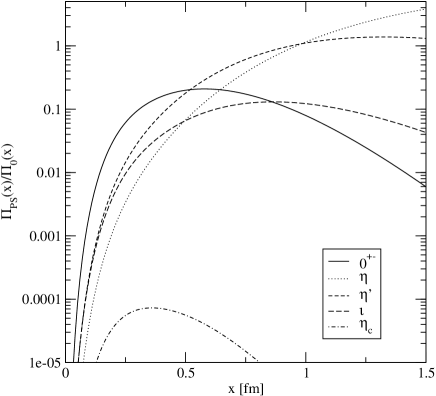
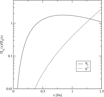
Figure 2.4: Resonance contributions to the pseudoscalar glueball correlation function $\langle g^{2}G\tilde{G}(0)g^{2}G\tilde{G}(x)\rangle$ and the charmonium correlator $\langle\bar{c}\gamma_{5}c(0)\bar{c}\gamma_{5}c(x)\rangle$. Both correlation functions are normalized to free field behavior. In the case of the gluonic correlation function we show the glueball contribution compared to the $\eta$, $\eta^{\prime}$, $\eta(1440)$ and $\eta_{c}$ contribution. For the charmonium correlation function we show the $\eta_{c}$ and glueball contribution.

We now proceed to the calculation of the exclusive decay rates. There are four final states that contribute to the $K\bar{K}\pi$ channel, $\eta_{c}\to K^{+}K^{-}\pi^{0}$, $K^{0}\bar{K}^{0}\pi^{0}$, $K^{+}\bar{K}^{0}\pi^{-}$ and $K^{-}K^{0}\pi^{+}$. Using isospin symmetry it is sufficient to calculate only one of the amplitudes. Fierz rearranging equ. (2.4) we get the interaction responsible for the $\eta_{c}\to K^{+}K^{-}\pi^{0}$

$${\cal L}_{I+A}^{K^{+}K^{-}\pi^{0}} = \int dz\int\frac{d\rho}{\rho^{5}}d_{0}(\rho)\frac{1}{N_{c}^{2}-1}\left(\frac{\pi^{3}\rho^{4}}{\alpha_{s}^{2}}\right)\left(\frac{4}{3}\pi^{2}\rho^{3}\right)^{3}$$ (2.28)

$$\times\frac{1}{4}(\alpha_{s}G\tilde{G})(\bar{s}\gamma^{5}u)(\bar{u}\gamma^{5}s)(\bar{d}\gamma^{5}d).$$

The decay rate is given by

$$\Gamma_{K^{+}K^{-}\pi^{0}}=\int({\rm phase\;\;space})\times|M|^{2}=\left[\frac{1}{16\pi\sqrt{2}}A\lambda_{\eta_{c}}K_{\pi}K_{K}^{2}\right]^{2}\times\left(0.111\,{\rm MeV}\right),$$ (2.29)

with $A$ given in equ. (2.14). Isospin symmetry implies that the other $K\bar{K}\pi$ decay rates are given by

$$\Gamma_{K^{+}K^{-}\pi^{0}}=\Gamma_{K^{0}\bar{K}^{0}\pi^{0}}=\left(\frac{1}{\sqrt{2}}\right)^{2}\Gamma_{K^{0}K^{-}\pi^{+}}=\left(\frac{1}{\sqrt{2}}\right)^{2}\Gamma_{K^{+}\bar{K}^{0}\pi^{-}}.$$ (2.30)

The total $K\bar{K}\pi$ decay rate is

$$\Gamma_{K\bar{K}\pi}=6\times\left[\frac{1}{16\pi\sqrt{2}}A\lambda_{\eta_{c}}K_{\pi}K_{K}^{2}\right]^{2}\times\left(0.111\,{\rm MeV}\right).$$ (2.31)

In a similar fashion we obtain

$$\Gamma_{\eta\pi\pi} = \frac{3}{2}\times\left[\frac{1}{16\pi}A\lambda_{\eta_{c}}K_{\eta}^{s}K_{\pi}^{2}\right]^{2}\times\left(0.135\,{\rm MeV}\right),$$ (2.32)

$$\Gamma_{\eta^{\prime}\pi\pi} = \frac{3}{2}\times\left[\frac{1}{16\pi}A\lambda_{\eta_{c}}K_{\eta^{\prime}}^{s}K_{\pi}^{2}\right]^{2}\times\left(0.0893\,{\rm MeV}\right),$$ (2.33)

$$\Gamma_{K\bar{K}\eta} = 2\times\left[\frac{1}{16\pi}A\lambda_{\eta_{c}}K_{\eta}^{q}K_{K}^{2}\right]^{2}\times\left(0.0788\,{\rm MeV}\right),$$ (2.34)

$$\Gamma_{K\bar{K}\eta^{\prime}} = 2\times\left[\frac{1}{16\pi}A\lambda_{\eta_{c}}K_{\eta^{\prime}}^{q}K_{K}^{2}\right]^{2}\times\left(0.0423\,{\rm MeV}\right),$$ (2.35)

$$\Gamma_{\eta\eta\eta} = \frac{1}{6}\times\left[\frac{3!}{16\pi}A\lambda_{\eta_{c}}(K_{\eta}^{q})^{2}K_{\eta}^{s}\right]^{2}\times\left(0.0698\,{\rm MeV}\right).$$ (2.36)

Here, the first factor is the product of the isospin and final state symmetrization factors. The second factor is the amplitude and the third factor is the phase-space integral.

Figure 2.5: Decay widths $\eta_{c}\to KK\pi$ and $\eta_{c}\to\eta\pi\pi$ as a function of the average instanton size $\rho$. The short dashed line shows the experimental $KK\pi$ width.

In Fig. 2.5 we show the dependence of the decay rates on the average instanton size. We observe that the experimental $K\bar{K}\pi$ rate is reproduced for $\bar{\rho}=0.29$ fm. This number is consistent with the phenomenological instanton size. However, given the strong dependence on the average instanton size it is clear that we cannot reliably predict the decay rate. On the other hand, the following ratios are independent of the average instanton size

$$\frac{\Gamma_{K\bar{K}\pi}}{\Gamma_{\eta\pi\pi}} = 4\times\left[\frac{K_{K}^{2}}{\sqrt{2}K_{\eta}^{s}K_{\pi}}\right]^{2}\times\left(\frac{0.111}{0.135}\right)=4.23\pm 1.27,$$ (2.37)

$$\frac{\Gamma_{\eta\pi\pi}}{\Gamma_{\eta^{\prime}\pi\pi}} = \left(\frac{K_{\eta}^{s}}{K_{\eta^{\prime}}^{s}}\right)^{2}\times\left(\frac{0.135}{0.0893}\right)=1.01,$$ (2.38)

$$\frac{\Gamma_{K\bar{K}\eta}}{\Gamma_{K\bar{K}\pi}} = \frac{1}{3}\times\left[\frac{\sqrt{2}K_{\eta}^{q}}{K_{\pi}}\right]^{2}\times\left(\frac{0.0788}{0.111}\right)=0.141\pm 0.042,$$ (2.39)

$$\frac{\Gamma_{K\bar{K}\eta}}{\Gamma_{K\bar{K}\eta^{\prime}}} = \left(\frac{K_{\eta}^{q}}{K_{\eta^{\prime}}^{q}}\right)^{2}\times\left(\frac{0.0788}{0.0423}\right)=2.91,$$ (2.40)

$$\frac{\Gamma_{\eta\eta\eta}}{\Gamma_{K\bar{K}\pi}} = \frac{1}{36}\times\left[\frac{3!\sqrt{2}(K_{\eta}^{q})^{2}K_{\eta}^{s}}{K_{\pi}K_{K}^{2}}\right]^{2}\times\left(\frac{0.0698}{0.111}\right)=0.011\pm 0.003,$$ (2.41)

where we have only quoted the error due to the uncertainty in $m_{s}$. These numbers should be compared to the experimental results

$$\left.\frac{\Gamma_{K\bar{K}\pi}}{\Gamma_{\eta\pi\pi}}\right|_{exp} = 1.1\pm 0.5$$ (2.42)

$$\left.\frac{\Gamma_{\eta\pi\pi}}{\Gamma_{\eta^{\prime}\pi\pi}}\right|_{exp} = 1.2\pm 0.6.$$ (2.43)

We note that the ratio $B(\eta\pi\pi)/B(\eta^{\prime}\pi\pi)$ is compatible with our results while the ratio $B(K\bar{K}\pi)/B(\eta\pi\pi)$ is not. This implies that either there are contributions other than instantons, or that the PCAC estimate of the ratio of coupling constants is not reliable, or that the experimental result is not reliable. The branching ratios for $\eta\pi\pi$ and $\eta^{\prime}\pi\pi$ come from MARK II/III experiments [46, 47]. We observe that our results for $B(K\bar{K}\eta)/B(K\bar{K}\pi)$ and $B(K\bar{K}\eta^{\prime})/B(K\bar{K}\pi)$ are consistent with the experimental bounds.

Another possibility is that there is a significant contribution from a scalar resonance that decays into $\pi\pi$. Indeed, instantons couple strongly to the $\sigma(600)$ resonance, and this state is not resolved in the experiments. We have therefore studied the direct instanton contribution to the decay $\eta_{c}\to\sigma\eta$. After Fierz rearrangement we get the effective vertex

$${\cal L}_{\sigma\eta} = \int dA\;(\alpha_{s}G\tilde{G})\;\frac{1}{4}\left[(\bar{u}\gamma^{5}u)(\bar{d}d)(\bar{s}{s})+(\bar{u}u)(\bar{d}\gamma^{5}d)(\bar{s}{s})+(\bar{u}u)(\bar{d}d)(\bar{s}\gamma^{5}{s})\right]$$ (2.44)

$$\mbox{}-\int dB\;m_{s}(\alpha_{s}G\tilde{G})\;\frac{1}{2}\left[(\bar{u}\gamma^{5}u)(\bar{d}d)+(\bar{u}u)(\bar{d}\gamma^{5}d)\right],$$

where the integrals $A$ and $B$ are defined in equ. (2.14,2.20). The only new matrix element we need is $f_{\sigma}=\langle\sigma|\bar{u}u+\bar{d}d|0\rangle\simeq(500\,{\rm MeV})^{2}$ [48]. We get

$$\Gamma_{\eta_{c}\to\sigma\eta} = \frac{1}{16\pi m_{\eta_{c}}^{3}}\sqrt{[m_{\eta_{c}}^{2}-(m_{\sigma}+m_{\eta})^{2}][m_{\eta_{c}}^{2}-(m_{\sigma}-m_{\eta})^{2}]}$$ (2.45)

$$\times\left[\frac{1}{16\pi}f_{\sigma}\lambda_{\eta_{c}}[(AQ_{s}-2Bm_{s})K_{\eta}^{q}+AK_{\eta}^{s}Q_{d}]\right]^{2}.$$

Compared to the direct decay $\eta_{c}\to\eta\pi\pi$ the $\eta_{c}\to\eta\sigma$ channel is suppressed by a factor $\sim(2\pi^{2}/m_{\eta_{c}}^{2})\cdot(Q_{q}f_{\sigma}/K_{\pi}^{2})^{2}\sim 1/100$. Here, the first factor is due to the difference between two and three-body phase space and the second factor is the ratio of matrix elements. We conclude that the direct production of a $\sigma$ resonance from the instanton does not give a significant contribution to $\eta_{c}\to\eta(\eta^{\prime})\pi\pi$. This leaves the possibility that the $\pi\pi$ channel is enhanced by final state interactions.

Figure 2.6: The Feynman diagram corresponding to the perturbative treatment of charmonium decay.

Finally, we present a perturbative estimate of the coupling of the $\eta_{c}$ to the instanton. We follow the method used by Anselmino and Forte in order to estimate the instanton contribution to $\eta_{c}\to p\bar{p}$ [49]. The idea is that the charmonium state annihilates into two gluons which are absorbed by the instanton. The Feynman diagram for the process is shown in Fig.2.6. The amplitude is given by

$$A_{c\bar{c}\to I} = g^{2}\int\frac{d^{4}k_{1}}{(2\pi)^{4}}\int\frac{d^{4}k_{2}}{(2\pi)^{4}}\,(2\pi)^{4}\delta^{4}(p_{1}+p_{2}-k_{1}-k_{2})\times$$ (2.46)

$$\bar{v}(p_{2})\left[\gamma_{\mu}\frac{\lambda^{a}}{2}\frac{1}{{p\!\!\!/}_{1}-{k\!\!\!/}_{1}-m_{c}}\gamma_{\nu}\frac{\lambda^{b}}{2}\right]u(p_{1})\;A_{\mu}^{a,cl}(k_{2})A_{\nu}^{b,cl}(k_{1}),$$

where $u(p)$ and $\bar{v}(p)$ are free particle charm quark spinors and $A_{\mu}^{a,cl}(k)$ is the Fourier transform of the instanton gauge potential

$$A_{\mu}^{a,cl}(k)=-i\frac{4\pi^{2}}{g}\frac{\bar{\eta}^{a}_{\mu\nu}k^{\nu}}{k^{4}}\Phi(k),\hskip 28.45274pt\Phi(k)=4\left(1-\frac{1}{2}K_{2}(k\rho)(k\rho)^{2}\right).$$ (2.47)

The amplitude for the charmonium state to couple to an instanton is obtained by folding equ. (2.46) with the $\eta_{c}$ wave function $\psi(p)$. In the non-relativistic limit the amplitude only depends on the wave function at the origin.

The perturbative estimate of the transition rate is easily incorporated into the results obtained above by replacing the product $A\lambda_{\eta_{c}}$ in equs. (2.29-2.36) according to

$$A\lambda_{\eta_{c}}\to\int\frac{d\rho}{\rho^{5}}d_{0}(\rho)\left(\frac{4}{3}\pi^{2}\rho^{3}\right)^{3}\left(4\pi\right)\frac{8m_{c}^{3/2}}{\sqrt{6}}|\psi(0)|I_{\eta_{c}}(\rho)\times\frac{g^{2}(m_{c}^{-1})}{g^{2}(\rho)},$$ (2.48)

with

$$I_{\eta_{c}}(\rho)=\int d^{4}k\;\frac{\vec{k}^{2}\Phi(k)\Phi(k-2p_{c})}{k^{4}(k-2p_{c})^{4}((k-p_{c})^{2}+m_{c}^{2})}.$$ (2.49)

Here, $p_{c}=(m_{c},0)\simeq(M_{\eta_{c}}/2,0)$ is the momentum of the charm quark in the charmonium rest frame. We note that because of the non-perturbative nature of the instanton field higher order corrections to equ. (2.48) are only suppressed by $g^{2}(m_{c}^{-1})/g^{2}(\rho)$.

The integral $I_{\eta_{c}}$ cannot be calculated analytically. We use the parameterization

$$I_{\eta_{c}}(\rho)\simeq\frac{\pi^{2}\;A_{0}\;\rho^{4}\log(1+1/(m_{c}\rho))}{1+B_{0}\;(m_{c}\rho)^{4}\log(1+1/(m_{c}\rho))},$$ (2.50)

which incorporates the correct asymptotic behavior. We find that $A_{0}=0.213$ and $B_{0}=0.124$ provides a good representation of the integral. In Fig. 2.7 we show the results for the $\eta_{c}$ decay rates as a function of the average instanton size. We observe that the results are similar to the results obtained from the phenomenological estimate equ. (2.27). The effective coupling $(A\lambda_{\eta_{c}})$ differs from the estimate equ. (2.27) by about a factor of 3. The experimental $K\bar{K}\pi$ rate is reproduced for $\bar{\rho}=0.31$ fm.

Figure 2.7: Decay rates $\Gamma(\eta_{c}\to K\bar{K}\pi)$ and $\Gamma(\eta_{c}\to\eta\pi\pi)$ as a function of the average instanton size $\bar{\rho}$. We show both the results from a phenomenological and a perturbative estimate of the $\bar{c}c$ coupling to the instanton.

2.5 Chi charm decays

Another interesting consistency check on our results is provided by the study of instanton induced decays of the $\chi_{c}$ into pairs of Goldstone bosons. The $\chi_{c}$ is a scalar charmonium bound state with mass $m_{\chi_{c}}=3415$ MeV and width $\Gamma_{\chi_{c}}=14.9$ MeV. In a potential model the $\chi_{c}$ corresponds to the ${}^{3}P_{0}$ state. In perturbation theory the total decay rate is dominated by $\bar{c}c\to 2g$. The main exclusive decay channels are $\chi_{c}\to 2(\pi^{+}\pi^{-})$ and $\chi_{c}\to\pi^{+}\pi^{-}K^{+}K^{-}$ with branching ratios $(2.4\pm 0.6)\%$ and $(1.8\pm 0.6)\%$, respectively. It would be very interesting to know whether these final states are dominated by scalar resonances. We will concentrate on final states containing two pseudoscalar mesons. There are two channels with significant branching ratios, $\chi_{c}\to\pi^{+}\pi^{-}$ and $\chi_{c}\to K^{+}K^{-}$ with branching ratios $(5.0\pm 0.7)\cdot 10^{-3}$ and $(5.9\pm 0.9)\cdot 10^{-3}$.

The calculation of these two decay rates proceeds along the same lines as the calculation of the $0^{++}$ glueball decays. The only new ingredient is the $\chi_{c}$ coupling to the gluon field strength $G^{2}$. We observe that the total $\chi_{c}$ decay rate implies that $\langle 0|2m_{c}\bar{c}c|\chi_{c}\rangle=3.1\,{\rm GeV}^{3}\simeq\langle 0|2m_{c}\bar{c}i\gamma_{5}c|\eta_{c}\rangle$. This suggests that a rough estimate of the $\chi_{c}$ coupling to $G^{2}$ is given by

$$\lambda_{\chi_{c}}\equiv\langle\chi_{c}|g^{2}G^{2}|0\rangle\simeq\lambda_{\eta_{c}}=1.12\;{\rm GeV}^{3}.$$ (2.51)

Using this result we can obtain the $\chi_{c}$ decay rates by rescaling the scalar glueball decay rates equ. (2.3-2.3) according to

$$\Gamma_{\chi_{c}\rightarrow m1,m2}=\Gamma_{0^{++}\rightarrow m1,m2}\times\left.\left(\frac{\lambda_{\chi_{c}}}{\lambda_{0^{++}}}\right)^{2}\right|_{m_{0^{++}}\to m_{\chi_{c}}},$$ (2.52)

where $m1,m2$ labels the two-meson final state. In Fig. 2.8 we show the dependence of the $\chi_{c}$ decay rates on the average instanton size $\bar{\rho}$. We observe that the experimental $\pi^{+}\pi^{-}$ decay rate is reproduced for $\bar{\rho}=0.29$ fm. In Fig. 2.9 we plot the ratio of decay rates for $\pi^{+}\pi^{-}$ and $K^{+}K^{-}$. Again, the experimental value is reproduced for $\bar{\rho}\sim 0.3$ fm.

Figure 2.8: Decay widths $\chi_{c}\to K^{+}K^{-},\pi^{+}\pi^{-}$ and $\eta\eta$ as a function of the average instanton size $\rho$. The short dashed line shows the experimental $K^{+}K^{-}$ width.

Figure 2.9: Ratio $B(\chi_{c}\to\pi^{+}\pi^{-})/B(\chi_{c}\to K^{+}K^{-})$ of decay rates as a function of the average instanton size. The dashed line shows the experimental value 0.84. We also show the experimental uncertainty, as well as the uncertainty in the instanton prediction due to the the value of the strange quark mass.

Finally, we can also estimate the $c\bar{c}$ coupling to the instanton using the perturbative method introduced in section 2.4. In the case of the $\chi_{c}$ we use

$$\frac{1}{4\pi}\lambda_{\chi_{c}}A \rightarrow \frac{1}{2\sqrt{3\pi}}\sqrt{M_{\chi}}R^{\prime}(0)\int\frac{d_{0}(\rho)}{\rho^{5}}d\rho\left(\frac{4}{3}\pi^{2}\rho^{3}\right)^{3}\frac{g^{2}(m_{c})}{g^{2}(\rho)}\times I_{\chi}(\rho),$$

$$\frac{1}{4\pi}\lambda_{\chi_{c}}B \rightarrow \frac{1}{2\sqrt{3\pi}}\sqrt{M_{\chi}}R^{\prime}(0)\int\frac{d_{0}(\rho)}{\rho^{5}}d\rho\left(\frac{4}{3}\pi^{2}\rho^{3}\right)^{2}\rho\,\frac{g^{2}(m_{c})}{g^{2}(\rho)}\times I_{\chi}(\rho)\>,$$

where $R^{\prime}(0)\simeq 0.39\,{\rm GeV}^{5/2}$ is the derivative of the ${}^{3}P_{0}$ wave function at the origin and $I_{\chi_{c}}$ is the loop integral

$$I_{\chi}(\rho)=\int\!d^{4}k\>\frac{\Phi(k)\Phi(|2p_{c}-k|)}{k^{4}(2p_{c}-k)^{4}}\>\>\frac{15(k-p_{c})^{2}+3m_{c}^{2}+4\vec{k}^{2}}{(k-p_{c})^{2}+m_{c}^{2}}.$$ (2.53)

In Fig. 2.10 we compare the perturbative result with the phenomenological estimate. Again, the results are comparable. The experimental $\pi^{+}\pi^{-}$ rate is reproduced for $\bar{\rho}=0.29$ fm.

Figure 2.10: Decay rates $\Gamma(\chi_{c}\to\pi^{+}\pi^{-})$ and $\Gamma(\chi_{c}\to K^{+}K^{-})$ as a function of the average instanton size $\bar{\rho}$. We show both the results from a phenomenological and a perturbative estimate of the $\bar{c}c$ coupling to the instanton.

2.6 Conclusions

In summary we have studied the instanton contribution to the decay of a number of “gluon rich” states in the (1.5-3.5) GeV range, the scalar glueball, the $\eta_{c}$ and the $\chi_{c}$. In the case of charmonium instanton induced decays are probably a small part of the total decay rate, but the final states are very distinctive. In the case of the scalar glueball classical fields play an important role in determining the structure of the bound state and instantons may well dominate the total decay rate.

We have assumed that the gluonic system is small and that the instanton contribution to the decay can be described in terms of an effective local interaction. The meson coupling to the local operator was determined using PCAC. Using this method we find that the scalar glueball decay is dominated by the $K\bar{K}$ final state for glueball masses $m_{0^{++}}>1$ GeV. In the physically interesting mass range $1.5\,{\rm GeV}<m_{0^{++}}<1.75\,{\rm GeV}$ the branching ratios satisfy $B(\eta\eta):B(\pi\pi):B(\bar{K}K)=1:(3.3\pm 0.3):(5.5\pm 0.5)$.

Our main focus in this work are $\eta_{c}$ decays into three pseudoscalar Goldstone bosons. We find that the experimental decay rate $\Gamma(\eta_{c}\to K\bar{K}\pi)$ can be reproduced for an average instanton size $\bar{\rho}=0.31$, consistent with phenomenological determinations and lattice results. This in itself is quite remarkable, since the phenomenological determination is based on properties of the QCD vacuum.

The ratio of decay rates $B(\eta^{\prime}\pi\pi):B(\eta\pi\pi):B(K\bar{K}\pi)=1:1:(4.2\pm 1.3)$ is insensitive to the average instanton size. While the ratio $B(\eta^{\prime}\pi\pi):B(\eta\pi\pi)=1:1$ is consistent with experiment, the ratio $B(\eta\pi\pi):B(K\bar{K})=1:(4.2\pm 1.3)$ is at best marginally consistent with the experimental value $1.1\pm 0.5$. We have also studied $\chi_{c}$ decays into two pseudoscalars. We find that the absolute decay rates can be reproduced for $\bar{\rho}=0.29$ fm. Instantons are compatible with the measured ratio $B(K^{+}K^{-}):B(\pi^{+}\pi^{-})=1.2$

There are many questions that remain to be answered. On the experimental side it would be useful if additional data for the channels $\eta_{c}\to\eta^{\prime}\pi\pi,\eta\pi\pi$ were collected. One important question is whether $(\pi\pi)$ resonances are important. It should also be possible to identify the smaller decay channels $\eta_{c}\to K\bar{K}\eta,K\bar{K}\eta^{\prime}$. In addition to that, it is interesting to study the distribution of the final state mesons in all three-meson channels. Instantons predict that the production mechanism is completely isotropic and that the final state mesons are distributed according to three-body phase space.

In addition to that, there are a number of important theoretical issues that remain to be resolved. In the limit in which the scalar glueball is light the decay $0^{++}\to\pi\pi(\bar{K}K)$ can be studied using effective lagrangians based on broken scale invariance [50, 51, 52]. Our calculation based on direct instanton effects is valid in the opposite limit. Nevertheless, the instanton liquid model respects Ward identities based on broken scale invariance [24] and one should be able to recover the low energy theorem. In the case $0^{++}\to\pi\pi(\bar{K}K)$ one should also be able to study the validity of the PCAC approximation in more detail. This could be done, for example, using numerical simulations of the instanton liquid. Finally we need to address the question how to properly compute the overlap of the initial $\bar{c}c$ system with the instanton. This, of course, is a more general problem that also affects calculations of electroweak baryon number violation in high energy $p\bar{p}$ collisions [53, 54] and QCD multi-particle production in hadronic collisions [55].

Chapter 3 Instantons and the spin of the nucleon

3.1 Introduction

In this chapter we will try to understand whether the so-called ”nucleon spin crises” can be related to instanton effects. The current interest in the spin structure of the nucleon dates from the 1987 discovery by the European Muon Collaboration that only about 30% of the spin of the proton is carried by the spin of the quarks [56]. This result is surprising from the point of view of the naive quark model, and it implies a large amount of OZI (Okubo-Zweig-Iizuka rule) violation in the flavor singlet axial vector channel. The axial vector couplings of the nucleon are related to polarized quark densities by

$$g_{A}^{3} = \Delta u-\Delta d,$$ (3.1)

$$g_{A}^{8} = \Delta u+\Delta d-2\Delta s,$$ (3.2)

$$g_{A}^{0} \equiv \Delta\Sigma=\Delta u+\Delta d+\Delta s.$$ (3.3)

The first linear combination is the well known axial vector coupling measured in neutron beta decay, $g_{A}^{3}=1.267\pm 0.004$. The hyperon decay constant is less well determined. A conservative estimate is $g_{A}^{8}=0.57\pm 0.06$. Polarized deep inelastic scattering is sensitive to another linear combination of the polarized quark densities and provides a measurement of the flavor singlet axial coupling constant $g_{A}^{0}$. Typical results are in the range $g_{A}^{0}=(0.28-0.41)$, see [57] for a recent review.

Since $g_{A}^{0}$ is related to the nucleon matrix element of the flavor singlet axial vector current many authors have speculated that the small value of $g_{A}^{0}$ is in some way connected to the axial anomaly, see [58, 59, 60] for reviews. The axial anomaly relation

$$\partial^{\mu}A_{\mu}^{0}=\frac{N_{f}g^{2}}{16\pi^{2}}G_{\mu\nu}^{a}\tilde{G}_{\mu\nu}^{a}+\sum_{f}2m_{f}\bar{q}_{f}i\gamma_{5}q_{f}$$ (3.4)

implies that matrix elements of the flavor singlet axial current $A_{\mu}^{0}$ are related to matrix elements of the topological charge density. The anomaly also implies that there is a mechanism for transferring polarization from quarks to gluons. In perturbation theory the nature of the anomalous contribution to the polarized quark distribution depends on the renormalization scheme. The first moment of the polarized quark density in the modified minimal subtraction $(\overline{MS})$ scheme is related to the first moment in the Adler-Bardeen $(AB)$ scheme by [61]

$$\Delta\Sigma_{\overline{MS}}=\Delta\Sigma_{AB}-N_{f}\frac{\alpha_{s}(Q^{2})}{2\pi}\Delta G(Q^{2}),$$ (3.5)

where $\Delta G$ is the polarized gluon density. Several authors have suggested that $\Delta\Sigma_{AB}$ is more naturally associated with the “constituent” quark spin contribution to the nucleon spin, and that the smallness of $\Delta\Sigma_{\overline{MS}}$ is due to a cancellation between $\Delta\Sigma_{AB}$ and $\Delta G$. The disadvantage of this scheme is that $\Delta\Sigma_{AB}$ is not associated with a gauge invariant local operator [62].

Non-perturbatively the anomaly implies that $g_{A}^{0}=\Delta\Sigma$ can be extracted from nucleon matrix elements of the pseudoscalar density $m\bar{\psi}i\gamma_{5}\psi$ and the topological charge density $g^{2}G^{a}_{\mu\nu}\tilde{G}^{a}_{\mu\nu}/(32\pi^{2})$ . The nucleon matrix element of the topological charge density is not known, but the matrix element of the scalar density $g^{2}G^{a}_{\mu\nu}G^{a}_{\mu\nu}$ is fixed by the trace anomaly. We have [63]

$$\langle N(p)|\frac{g^{2}}{32\pi^{2}}G^{a}_{\mu\nu}G^{a}_{\mu\nu}|N(p^{\prime})\rangle=C_{S}(q^{2})m_{N}\bar{u}(p)u(p^{\prime}),$$ (3.6)

with $C_{S}(0)=-1/b$ where $b=11-2N_{f}/3$ is the first coefficient of the QCD beta function. Here, $u(p)$ is a free nucleon spinor. Anselm suggested that in an instanton model of the QCD vacuum the gauge field is approximately self-dual, $G^{2}=\pm G\tilde{G}$, and the nucleon coupling constants of the scalar and pseudoscalar gluon density are expected to be equal, $C_{S}(0)\simeq C_{P}(0)$ [64], see also [65]. Using $g_{A}^{0}=N_{f}C_{P}(0)$ in the chiral limit we get $g_{A}^{0}\simeq-N_{f}/b\simeq-0.2$, which is indeed quite small.

A different suggestion was made by Narison, Shore, and Veneziano [66]. Narison et al. argued that the smallness of $\Delta\Sigma=g_{A}^{0}$ is not related to the structure of the nucleon, but a consequence of the $U(1)_{A}$ anomaly and the structure of the QCD vacuum. Using certain assumptions about the nucleon-axial-vector current three-point function they derive a relation between the singlet and octet matrix elements,

$$g_{A}^{0}=g_{A}^{8}\frac{\sqrt{6}}{f_{\pi}}\sqrt{\chi^{\prime}_{top}(0)}.$$ (3.7)

Here, $f_{\pi}=93$ MeV is the pion decay constant and $\chi^{\prime}_{top}(0)$ is the slope of the topological charge correlator

$$\chi_{top}(q^{2})=\int d^{4}x\,e^{iqx}\,\langle Q_{top}(0)Q_{top}(x)\rangle,$$ (3.8)

with $Q_{top}(x)=g^{2}G^{a}_{\mu\nu}\tilde{G}^{a}_{\mu\nu}/(32\pi^{2})$. In QCD with massless fermions topological charge is screened and $\chi_{top}(0)=0$. The slope of the topological charge correlator is proportional to the screening length. In QCD we expect the inverse screening length to be related to the $\eta^{\prime}$ mass. Since the $\eta^{\prime}$ is heavy, the screening length is short and $\chi^{\prime}_{top}(0)$ is small. Equation (3.7) relates the suppression of the flavor singlet axial charge to the large $\eta^{\prime}$ mass in QCD.

Both of these suggestions are very interesting, but the status of the underlying assumptions is somewhat unclear. In this work we would like to address the role of the anomaly in the nucleon spin problem, and the more general question of OZI violation in the flavor singlet axial-vector channel, by computing the axial charge of the nucleon and the axial-vector two-point function in the instanton model. There are several reasons why instantons are important in the spin problem. First of all, instantons provide an explicit, weak coupling, realization of the anomaly relation equ. (3.4) and the phenomenon of topological charge screening [24, 67]. Second, instantons provide a successful phenomenology of OZI violation in QCD [68]. Instantons explain, in particular, why violations of the OZI rule in scalar meson channels are so much bigger than OZI violation in vector meson channels. And finally, the instanton liquid model gives a very successful description of baryon correlation functions and the mass of the nucleon [69, 70].

Our ideas are organized as follows. In Sect. 3.2 we review the calculation of the anomalous contribution to the axial-vector current in the field of an instanton. In Sect. 3.3 and 3.4 we use this result in order to study OZI violation in the axial-vector correlation function and the axial coupling of a constituent quark. Our strategy is to compute the short distance behavior of the correlation functions in the single instanton approximation and to determine the large distance behavior using numerical simulations. In Sect. 3.5 we present numerical calculations of the axial couplings of the nucleon and in Sect. 3.6 we discuss our conclusions. Some results regarding the spectral representation of nucleon three-point functions are collected in appendix 6.1.

3.2 Axial Charge Violation in the Field of an Instanton

We would like to start by showing explicitly how the axial anomaly is realized in the field of an instanton. This discussion will be useful for the calculation of the OZI violating part of the axial-vector correlation function and the axial charge of the nucleon. The flavor singlet axial-vector current in a gluon background is given by

$$A_{\mu}(x)={\rm Tr}\left[\gamma_{5}\gamma_{\mu}S(x,x)\right]$$ (3.9)

where $S(x,y)$ is the full quark propagator in the background field. The expression on the right hand side of equ. (3.9) is singular and needs to be defined more carefully. We will employ a gauge invariant point-splitting regularization

$${\rm Tr}\left[\gamma_{5}\gamma_{\mu}S(x,x)\right]\equiv\lim_{\epsilon\to 0}{\rm Tr}\left[\gamma_{5}\gamma_{\mu}S(x+\epsilon,x-\epsilon)P\exp\left(-i\int_{x-\epsilon}^{x+\epsilon}A_{\mu}(x)dx\right)\right].$$ (3.10)

In the following we will consider an (anti) instanton in singular gauge. The gauge potential of an instanton of size $\rho$ and position $z=0$ is given by

$$A_{\mu}^{a}=\frac{2\rho^{2}}{x^{2}+\rho^{2}}\frac{x^{\nu}}{x^{2}}\,R^{ab}\bar{\eta}^{b}_{\mu\nu}.$$ (3.11)

Here, $\bar{\eta}^{a}_{\mu\nu}$ is the ’t Hooft symbol and $R^{ab}$ characterizes the color orientation of the instanton. The fermion propagator in a general gauge potential can be written as

$$S(x,y)=\sum_{\lambda}\frac{\Psi_{\lambda}(x)\Psi_{\lambda}^{+}(y)}{\lambda-m},$$ (3.12)

where $\Psi_{\lambda}(x)$ is a normalized eigenvector of the Dirac operator with eigenvalue $\lambda$, $D\!\!\!\!/\,\Psi_{\lambda}(x)=\lambda\Psi_{\lambda}(x)$. We will consider the limit of small quark masses. Expanding equ. (3.12) in powers of $m$ gives

$$S_{\pm}(x,y)=-\frac{\Psi_{0}(x)\Psi_{0}^{+}(y)}{m}+\sum_{\lambda\neq 0}\frac{\Psi_{\lambda}(x)\Psi_{\lambda}^{+}(y)}{\lambda}+m\sum_{\lambda\neq 0}\frac{\Psi_{\lambda}(x)\Psi_{\lambda}^{+}(y)}{\lambda^{2}}+O(m^{2}).$$ (3.13)

Here we have explicitly isolated the zero mode propagator. The zero mode $\Psi_{0}$ was found by ’t Hooft and is given by

$$\Psi_{0}(x)=\frac{\rho}{\pi}\frac{1}{(x^{2}+\rho^{2})^{3/2}}\frac{\gamma\cdot x}{\sqrt{x^{2}}}\gamma_{\pm}\phi.$$ (3.14)

Here, $\phi^{a\alpha}=\epsilon^{a\alpha}/\sqrt{2}$ is a constant spinor and $\gamma_{\pm}=(1\pm\gamma_{5})/2$ for an instanton/ anti-instanton. The second term in equ. (3.13) is the non-zero mode part of the propagator in the limit $m\to 0$ [71]

$$S_{\pm}^{NZ}(x,y)\equiv\sum_{\lambda\neq 0}\frac{\Psi_{\lambda}(x)\Psi_{\lambda}^{+}(y)}{\lambda}=\vec{D\!\!\!\!/\,}_{x}\Delta_{\pm}(x,y)\gamma_{\pm}+\Delta_{\pm}(x,y)\stackrel{{\scriptstyle\leftarrow}}{{D\!\!\!\!/\,}}_{y}\gamma_{\mp}$$ (3.15)

where $D^{\mu}=\partial^{\mu}-iA_{\pm}^{\mu}$ and $\Delta_{\pm}(x,y)$ is the propagator of a scalar field in the fundamental representation. Equ. (3.15) can be verified by checking that $S_{\pm}^{NZ}$ satisfies the equation of motion and is orthogonal to the zero mode. The scalar propagator can be found explicitly

$$\Delta_{\pm}(x,y)=\Delta_{0}(x,y)\frac{1}{\sqrt{1+\frac{\rho^{2}}{x^{2}}}}\left(1+\frac{\rho^{2}\sigma_{\mp}\cdot x\sigma_{\pm}\cdot y}{x^{2}y^{2}}\right)\frac{1}{\sqrt{1+\frac{\rho^{2}}{y^{2}}}},$$ (3.16)

where $\Delta_{0}=1/(4\pi^{2}\Delta^{2})$ with $\Delta=x-y$ is the free scalar propagator. The explicit form of the non-zero mode propagator can be obtained by substituting equ. (3.16) into equ. (3.15). We find

$$S^{NZ}_{\pm}(x,y) = \frac{1}{\sqrt{1+\frac{\rho^{2}}{x^{2}}}}\frac{1}{\sqrt{1+\frac{\rho^{2}}{y^{2}}}}\left\{S_{0}(x-y)\left(1+\frac{\rho^{2}\sigma_{\mp}\cdot x\sigma_{\pm}\cdot y}{x^{2}y^{2}}\right)\right.$$ (3.17)

$$\hskip 8.5359pt\mbox{}-\frac{\Delta_{0}(x-y)}{x^{2}y^{2}}\left(\frac{\rho^{2}}{\rho^{2}+x^{2}}\sigma_{\mp}\cdot x\sigma_{\pm}\cdot\gamma\sigma_{\mp}\cdot\Delta\sigma_{\pm}\cdot y\gamma_{\pm}\right.$$

$$\hskip 56.9055pt\mbox{}\left.\left.+\frac{\rho^{2}}{\rho^{2}+y^{2}}\sigma_{\mp}\cdot x\sigma_{\pm}\cdot\Delta\sigma_{\mp}\cdot\gamma\sigma_{\pm}\cdot y\gamma_{\mp}\right)\right\}$$

Here, $S_{0}=-\Delta\!\!\!//(2\pi^{2}\Delta^{4})$ denotes the free quark propagator. As expected, the full non-zero mode propagator reduces to the free propagator at short distance. The linear mass term in equ. (3.13) can be written in terms of the non-zero mode propagator

$$\sum_{\lambda\neq 0}\frac{\Psi_{\lambda}(x)\Psi_{\lambda}^{+}(y)}{\lambda^{2}}=\int d^{4}zS^{NZ}_{\pm}(x,z)S^{NZ}_{\pm}(z,y)=-\Delta_{\pm}(x,y)\gamma_{\pm}-\Delta^{M}_{\pm}(x,y)\gamma_{\mp},$$ (3.18)

where $\Delta_{\pm}(x,y)$ is the scalar propagator and $\Delta^{M}_{\pm}(x,y)=\langle x|(D^{2}+\sigma\cdot G/2)^{-1}|y\rangle$ is the propagator of a scalar particle with a chromomagnetic moment. We will not need the explicit form of $\Delta^{M}_{\pm}(x,y)$ in what follows. We are now in the position to compute the regularized axial current given in equ. (3.10). We observe that neither the free propagator nor the zero mode part will contribute. Expanding the non-zero mode propagator and the path ordered exponential in powers of $\epsilon$ we find

$${\rm Tr}\left[\gamma_{5}\gamma^{\mu}S(x,x)\right]=\pm\frac{2\rho^{2}x^{\mu}}{\pi^{2}(x^{2}+\rho^{2})^{3}},$$ (3.19)

which shows that instantons act as sources and sinks for the flavor singlet axial current. We can now compare this result to the anomaly relation equ. (3.4). The divergence of equ. (3.19) is given by

$$\partial^{\mu}A_{\mu}(x)=\pm\frac{2\rho^{2}}{\pi^{2}}\frac{4\rho^{2}-2x^{2}}{(x^{2}+\rho^{2})^{4}}.$$ (3.20)

The topological charge density in the field of an (anti) instanton is

$$\frac{g^{2}}{16\pi^{2}}G^{a}_{\mu\nu}\tilde{G}^{a}_{\mu\nu}=\pm\frac{12\rho^{4}}{\pi^{2}(x^{2}+\rho^{2})^{4}}.$$ (3.21)

We observe that the divergence of the axial current given in equ. (3.19) does not agree with the topological charge density. The reason is that in the field of an instanton the second term in the anomaly relation, which is proportional to $m\bar{\psi}\gamma_{5}\psi$, receives a zero mode contribution and is enhanced by a factor $1/m$. In the field of an (anti) instanton we find

$$2m\bar{\psi}i\gamma_{5}\psi=\mp\frac{4\rho^{2}}{\pi^{2}(x^{2}+\rho^{2})^{3}}.$$ (3.22)

Taking into account both equ. (3.21) and (3.22) we find that the anomaly relation (3.4) is indeed satisfied.

3.3 OZI Violation in Axial-Vector Two-Point Functions

In this section we wish to study OZI violation in the axial-vector channel due to instantons. We consider the correlation functions

$$\Pi_{\mu\nu}^{j}(x,y)=\langle j_{\mu}(x)j_{\nu}(y)\rangle,$$ (3.23)

where $j_{\mu}$ is one of the currents

$$\begin{array}[]{rcllrcll}V_{\mu}^{a}&=&\bar{\psi}\gamma_{\mu}\tau^{a}\psi&(\rho),&V_{\mu}^{0}&=&\bar{\psi}\gamma_{\mu}\psi&(\omega),\\ A_{\mu}^{a}&=&\bar{\psi}\gamma_{\mu}\gamma_{5}\tau^{a}\psi&(a_{1}),&A_{\mu}^{0}&=&\bar{\psi}\gamma_{\mu}\gamma_{5}\psi&(f_{1}),\end{array}$$ (3.24)

where in the brackets we have indicated the mesons with the corresponding quantum numbers. We will work in the chiral limit $m_{u}=m_{d}\to 0$. The iso-vector correlation functions only receive contributions from connected diagrams. The iso-vector vector ($\rho$) correlation function is

$$(\Pi_{V}^{3})_{\mu\nu}(x,y)=2(P^{con}_{V})_{\mu\nu}(x,y)=-2\langle{\rm Tr}\left[\gamma_{\mu}S(x,y)\gamma_{\nu}S(y,x)\right]\rangle.$$ (3.25)

The iso-singlet correlator receives additional, disconnected, contributions, see Fig. 3.1.

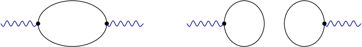
Figure 3.1: Quark line diagrams that contribute to the vector and axial-vector two-point function in the iso-vector and iso-singlet channel. The solid lines denote quark propagators in a gluonic background field. The two diagrams show the connected and disconnected contribution.

The iso-singlet vector ($\omega$) correlator is given by

$$(\Pi_{V}^{0})_{\mu\nu}(x,y)=2(P^{con}_{V})_{\mu\nu}(x,y)+4(P^{dis}_{V})_{\mu\nu}(x,y)$$ (3.26)

with

$$(P^{dis}_{V})_{\mu\nu}(x,y)=\langle{\rm Tr}\left[\gamma_{\mu}S(x,x)\right]{\rm Tr}\left[\gamma_{\nu}S(y,y)\right]\rangle.$$ (3.27)

The axial-vector correlation functions are defined analogously. At very short distance the correlation functions are dominated by the free quark contribution $\Pi_{A}^{3}=\Pi_{A}^{0}=\Pi_{V}^{3}=\Pi_{V}^{0}\sim 1/x^{6}$. Perturbative corrections to the connected correlators are $O(\alpha_{s}(x)/\pi)$, but perturbative corrections to the disconnected correlators are very small, $O((\alpha_{s}(x)/\pi)^{2})$. In this section we will compute the instanton contribution to the correlation functions. At short distance, it is sufficient to consider a single instanton. For the connected correlation functions, this calculation was first performed by Andrei and Gross [72], see also [73]. Disconnected correlation function were first considered in [74] and a more recent study can be found in [75].

In order to make contact with our calculation of the vector and axial-vector three-point functions in the next section, we briefly review the calculation of Andrei and Gross, and then compute the disconnected contribution. Using the expansion in powers of the quark mass, equ. (3.13), we can write

$$(P^{con}_{V})_{\pm}^{\mu\nu}(x,y)=(P^{con}_{V})^{\mu\nu}_{0}+A^{\mu\nu}_{\pm}+B^{\mu\nu}_{\pm}$$ (3.28)

with

$$(P_{V}^{con})^{\mu\nu}_{0} = -{\rm Tr}\left[\gamma^{\mu}S_{0}(x,y)\gamma^{\nu}S_{0}(y,x)\right],$$ (3.29)

$$A^{\mu\nu}_{\pm} = -{\rm Tr}\left[\gamma^{\mu}S^{NZ}_{\pm}(x,y)\gamma^{\nu}S^{NZ}_{\pm}(y,x)\right]-(P^{con}_{V})_{0}^{\mu\nu}(x,y),$$ (3.30)

$$B^{\mu\nu}_{\pm} = -2{\rm Tr}\left[\gamma^{\mu}\Psi_{0\pm}(x)\Psi_{0\pm}^{+}(y)\gamma^{\nu}\Delta_{\pm}(y,x)\gamma_{\pm}\right].$$ (3.31)

Using the explicit expression for the propagators given in the previous section we find

$$A^{\mu\nu}_{\pm} = \frac{\rho^{2}h_{x}h_{y}}{2\pi^{4}\Delta^{4}}\left\{S^{\mu\alpha\nu\beta}\Big{[}\rho^{2}h_{x}h_{y}(2\Delta_{\alpha}\Delta_{\beta}-\Delta^{2}\delta_{\alpha\beta})+h_{y}(y_{\beta}\Delta_{\alpha}+y_{\alpha}\Delta_{\beta})\right.$$ (3.32)

$$\hskip 28.45274pt\mbox{}\left.-h_{x}(x_{\beta}\Delta_{\alpha}+x_{\alpha}\Delta_{\beta})\Big{]}\mp 2\epsilon^{\mu\nu\alpha\beta}(h_{y}\Delta_{\alpha}y_{\beta}-h_{x}\Delta_{\beta}x_{\alpha})\right\}$$

and

$$B^{\mu\nu}_{\pm}=-\frac{\rho^{2}}{\pi^{4}\Delta^{2}}h_{x}^{2}h_{y}^{2}\left\{(x\cdot y+\rho^{2})\delta^{\mu\nu}-(y^{\mu}x^{\nu}-x^{\mu}y^{\nu})\mp\epsilon^{\mu\alpha\nu\beta}x_{\alpha}y_{\beta}\right\}$$ (3.33)

with $h_{x}=1/(x^{2}+\rho^{2})$, $\Delta=x-y$, and $S^{\mu\alpha\nu\beta}=g^{\mu\alpha}g^{\nu\beta}-g^{\mu\nu}g^{\alpha\beta}+g^{\mu\beta}g^{\alpha\nu}$. Our result agrees with [72] up to a color factor of $3/2$, first noticed in [76], a ’-’ sign in front of the epsilon terms, which cancels after adding instantons and anti-instantons, and a ’-’ sign in front of the 2nd term in $B^{\mu\nu}$. This sign is important in order to have a conserved current, but it does not affect the trace $P^{\mu\mu}$. Summing up the contributions from instantons and anti-instantons we obtain

$$(P^{con}_{V})^{\mu\nu}(x,y) = 2\frac{12S^{\mu\alpha\nu\beta}\Delta_{\alpha}\Delta_{\beta}}{(2\pi^{2})^{2}\Delta^{8}}+\frac{1}{2\pi^{4}}(h_{x}h_{y})^{2}\rho^{2}\left[-\frac{2\Sigma^{2}}{\Delta^{4}}\Delta^{\mu}\Delta^{\nu}\right.$$ (3.34)

$$+\frac{2\Sigma\cdot\Delta}{\Delta^{4}}(\Sigma^{\mu}\Delta^{\nu}+\Delta^{\mu}\Sigma^{\nu}-\Sigma\cdot\Delta g^{\mu\nu})$$

$$\left.+\frac{2}{\Delta^{2}}(\Delta^{2}g^{\mu\nu}-\Delta^{\mu}\Delta^{\nu}-\Delta^{\mu}\Sigma^{\nu}+\Delta^{\nu}\Sigma^{\mu})\right].$$

This result has to be averaged over the position of the instanton. We find

$$2a^{\mu\nu} = \sum_{\pm}\int d^{4}zA^{\mu\nu}_{\pm}(x-z,y-z)$$ (3.35)

$$= -\frac{1}{\pi^{2}}\left[\frac{\partial^{2}}{\partial\Delta_{\mu}\partial\Delta_{\nu}}G(\Delta^{2},\rho)+2G^{\prime}(\Delta^{2},\rho)g^{\mu\nu}\right],$$

$$2b^{\mu\nu} = \sum_{\pm}\int d^{4}zB^{\mu\nu}_{\pm}(x-z,y-z)=\frac{1}{\pi^{2}}\left[\frac{\partial^{2}}{\partial\Delta^{2}}G(\Delta^{2},\rho)+2G^{\prime}(\Delta^{2},\rho)\right]g^{\mu\nu},$$

with

$$G^{\prime}(\Delta^{2},\rho)=\frac{\partial G(\Delta^{2},\rho)}{\partial\Delta^{2}}=\frac{\rho^{2}}{\Delta^{4}}\left[-\frac{2\rho^{2}}{\Delta^{2}}\xi\log\frac{1-\xi}{1+\xi}-1\right]$$ (3.37)

and $\xi^{2}=\Delta^{2}/(\Delta^{2}+4\rho^{2})$. The final result for the single instanton contribution to the connected part of the vector current correlation function is

$$\delta(P_{V}^{con})^{\mu\mu} = (P_{V}^{con})^{\mu\mu}-2(P^{con}_{V})^{\mu\mu}_{0}=\frac{24}{\pi^{2}}\frac{\rho^{4}}{\Delta^{2}}\;\frac{\partial}{\partial\Delta^{2}}\left(\frac{\xi}{\Delta^{2}}\log\frac{1+\xi}{1-\xi}\right)$$ (3.38)

$$\equiv \frac{24}{\pi^{2}}\frac{\rho^{4}}{\Delta^{2}}F(\Delta,\xi),$$

where we defined

$$F(\Delta,\xi)=\frac{\partial}{\partial\Delta^{2}}\left(\frac{\xi}{\Delta^{2}}\log\frac{1+\xi}{1-\xi}\right).$$ (3.39)

The computation of the connected part of the axial-vector correlator is very similar. Using equs. (3.30,3.31) we observe that the only difference is the sign in front of $B^{\mu\nu}$. We find

$$\delta(P^{con}_{A})^{\mu\mu}=(P^{con}_{A})^{\mu\mu}-2(P^{con}_{A})^{\mu\mu}_{0}=-\frac{1}{\pi^{2}}\left[20\Delta^{2}G^{\prime\prime}+56G^{\prime}\right],$$ (3.40)

with $G^{\prime}$ given in equ. (3.37)

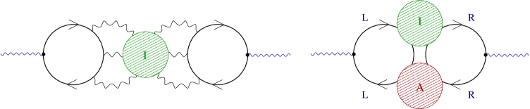
Figure 3.2: Instanton contributions to the disconnected axial-vector correlation function. The left panel shows the single-instanton (non-zero mode) contribution. The right panel shows the instanton-anti-instanton (fermion zero mode) contribution.

We now come to the disconnected part, see Fig. 3.2. In the vector channel the single instanton contribution to the disconnected correlator vanishes [74]. In the axial-vector channel we can use the result for ${\rm Tr}[\gamma_{5}\gamma^{\mu}S(x,x)]$ derived in the previous section. The correlation function is

$$(P^{dis}_{A})^{\mu\nu}(x,y)=\frac{4\rho^{4}(x-z)^{\mu}(y-z)^{\nu}}{\pi^{4}((x-z)^{2}+\rho^{2})^{3}((y-z)^{2}+\rho^{2})^{3}}.$$ (3.41)

Summing over instantons and anti-instantons and integrating over the center of the instanton gives

$$(P^{dis}_{A})^{\mu\nu}=2\frac{\rho^{4}}{2\pi^{2}}\frac{\partial^{2}}{\partial\Delta_{\mu}\partial\Delta_{\nu}}F(\Delta,\xi)$$ (3.42)

and

$$(P^{dis}_{A})^{\mu\mu}=\frac{4\rho^{4}}{\pi^{2}}\left\{2\frac{d}{d\Delta^{2}}+\Delta^{2}\left(\frac{d}{d\Delta^{2}}\right)^{2}\right\}F(\Delta,\xi).$$ (3.43)

We can now summarize the results in the vector singlet ($\omega$) and triplet ($\rho$), as well as axial-vector singlet ($f_{1}$) and triplet ($a_{1}$) channel. The result in the $\rho$ and $\omega$ channel is

$$(\Pi^{3}_{V})^{\mu\mu}=(\Pi^{0}_{V})^{\mu\mu}=-\frac{12}{\pi^{4}\Delta^{6}}+2\int d\rho n(\rho)\frac{24}{\pi^{2}}\frac{\rho^{4}}{\Delta^{2}}F(\Delta,\xi).$$ (3.44)

In the $a_{1},f_{1}$ channel we have

$$(\Pi^{3}_{A})^{\mu\mu} = -\frac{12}{\pi^{4}\Delta^{6}}+\int d\rho n(\rho)\left[-\frac{2}{\pi^{2}}\left(20\Delta^{2}G^{\prime\prime}+56G^{\prime}\right)\right],$$ (3.45)

$$(\Pi^{0}_{A})^{\mu\mu} = -\frac{12}{\pi^{4}\Delta^{6}}+\int d\rho n(\rho)\left[-\frac{2}{\pi^{2}}\left(20\Delta^{2}G^{\prime\prime}+56G^{\prime}\right)\right.$$ (3.46)

$$\hskip 71.13188pt\left.+\frac{16\rho^{4}}{\pi^{2}}\left(2F^{\prime}+\Delta^{2}F^{\prime\prime}\right)\right].$$

In order to obtain a numerical estimate of the instanton contribution we use a very simple model for the instanton size distribution, $n(\rho)=n_{0}\delta(\rho-\bar{\rho})$, with $\bar{\rho}=0.3$ fm and $n_{0}=0.5\,{\rm fm}^{-4}$. The results are shown in Fig. 3.3.

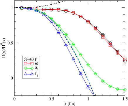
Figure 3.3: correlation functions in the $\rho,\omega,a_{1}$ and $f_{1}$ channel. All correlation functions are normalized to free field behavior. The data points show results from a numerical simulation of the random instanton liquid. The dashed lines show the single instanton approximation.

We observe that the OZI rule violating difference between the singlet and triplet axial-vector correlation functions is very small and repulsive. We can also see this by studying the short distance behavior of the correlation functions. The non-singlet correlators satisfy

$$(\Pi_{V}^{3})^{\mu\mu} = (\Pi_{V}^{3})^{\mu\mu}_{0}\left\{1+\frac{\pi^{2}x^{4}}{3}\int d\rho n(\rho)+\ldots\right\},$$ (3.47)

$$(\Pi_{A}^{3})^{\mu\mu} = (\Pi_{A}^{3})^{\mu\mu}_{0}\left\{1-\pi^{2}x^{4}\int d\rho n(\rho)+\ldots\right\}.$$ (3.48)

As explained by Dubovikov and Smilga, this result can be understood in terms of the contribution of the dimension $d=4$ operators $\langle g^{2}G^{2}\rangle$ and $\langle m\bar{q}q\rangle$ in the operator product expansion (OPE). The OZI violating contribution

$$(\Pi^{OZI}_{A})^{\mu\mu}=(\Pi^{0}_{A})^{\mu\mu}-(\Pi^{3}_{A})^{\mu\mu}=-(\Pi^{3}_{A})^{\mu\mu}_{0}\left(\frac{4\pi^{2}}{45}\frac{x^{6}}{\rho^{2}}\right)\int d\rho n(\rho)$$ (3.49)

is of $O(x^{6})$ and not singular at short distance. Our results show that it remains small and repulsive even if $x>\rho$. We also note that the sign of the OZI-violating term at short distance is model independent. The quark propagator in euclidean space satisfies the Weingarten relation

$$S(x,y)^{\dagger}=\gamma_{5}S(y,x)\gamma_{5}.$$ (3.50)

This relation implies that ${\rm Tr}[S(x,x)\gamma_{\mu}\gamma_{5}]$ is purely real. As a consequence we have

$$\lim_{x\to y}\Big{\{}{\rm Tr}[S(x,x)\gamma_{\mu}\gamma_{5}]{\rm Tr}[S(y,y)\gamma_{\mu}\gamma_{5}]\Big{\}}>0.$$ (3.51)

Since the path integral measure in euclidean space is positive this inequality translates into an inequality for the correlation functions. In our convention the trace of the free correlation function is negative, and equ. (3.51) implies that the interaction is repulsive at short distance. The result is in agreement with the single instanton calculation.

We can also study higher order corrections to the single instanton result. The two-instanton (anti-instanton) contributions is of the same form as the one-instanton result. An interesting contribution arises from instanton-anti-instanton pairs, see Fig. 3.2. This effect was studied in [77]. It was shown that the instanton-anti-instanton contribution to the disconnected meson channels can be described in terms of an effective lagrangian

$${\cal L}=\frac{2G}{N_{c}^{2}}(\bar{\psi}\gamma_{\mu}\gamma_{5}\psi)^{2}$$ (3.52)

with

$$G=\int d\rho_{1}d\rho_{2}(2\pi\rho_{1})^{2}(2\pi\rho_{2})^{2}\frac{n(\rho_{1},\rho_{2})}{8T_{IA}^{2}}$$ (3.53)

where $n(\rho_{1},\rho_{2})$ is the tunneling rate for an instanton-anti-instanton pair and $T_{IA}$ is the matrix element of the Dirac between the two (approximate) zero modes. We note that this interaction is also repulsive, and that there is no contribution to the $\omega$ channel.

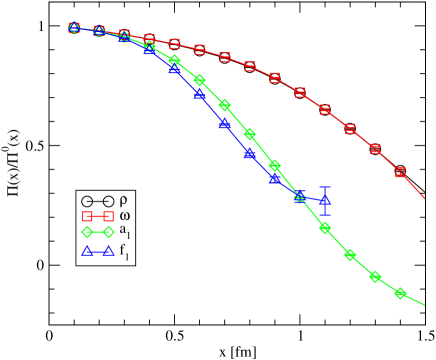
Figure 3.4: Correlation functions in the $\rho,\omega,a_{1}$ and $f_{1}$ channel. All correlation functions are normalized to free field behavior. The data points show results from unquenched simulations of the instanton liquid model.

Numerical results for the vector meson correlation functions are shown in Figs. 3.3 and 3.4. The correlation functions are obtained from Monte Carlo simulations of the instanton liquid as described in [78, 79]. We observe that OZI violation in the vector channel is extremely small, both in quenched and unquenched simulations. The OZI violating contribution to the $f_{1}$ channel is repulsive. In quenched simulations this contribution becomes sizable at large distance. Most likely this is due to mixing with an $\eta^{\prime}$ ghost pole. We observe that the effect disappears in unquenched simulations. The pion contribution to the $a_{1}$ correlator is of course present in both quenched and unquenched simulations.

Experimentally we know that the $\rho$ and $\omega$, as well as the $a_{1}$ and $f_{1}$ meson, are indeed almost degenerate. Both iso-singlet states are slightly heavier than their iso-vector partners. To the best of our knowledge there has been only one attempt to measure OZI violating correlation functions in the vector and axial-vector channel on the lattice, see [80]. Isgur and Thacker concluded that OZI violation in both channels was too small to be reliably measurable in their simulation.

3.4 Axial Vector Coupling of a Quark

In this section we wish to study the iso-vector and iso-singlet axial coupling of a single quark. Our purpose is twofold. One reason is that the calculation of the axial-vector three-point function involving a single quark is much simpler than that of the nucleon, and that it is closely connected to the axial-vector two-point function studied in the previous section. The second, more important, reason is the success of the constituent quark model in describing many properties of the nucleon. It is clear that constituent quarks have an intrinsic structure, and that the axial decay constant of a constituent quark need not be close to one. Indeed, Weinberg argued that the axial coupling of a quark is $(g_{A}^{3})_{Q}\simeq 0.8$ [81]. Using this value of $(g_{A}^{3})_{Q}$ together with the naive $SU(6)$ wave function of the nucleon gives the nucleon axial coupling $g_{A}^{3}=0.8\cdot 5/3\simeq 1.3$, which is a significant improvement over the naive quark model result $5/3$. It is interesting to study whether, in a similar fashion, the suppression of the flavor singlet axial charge takes place on the level of a constituent quark.

In order to address this question we study three-point functions involving both singlet and triplet vector and axial-vector currents. The vector three-point function is

$$(\Pi^{a}_{VQQ})^{\alpha\beta}_{\mu}(x,z,y)=\langle q^{\alpha}(x)V^{a}_{\mu}(z)\bar{q}^{\beta}(y)\rangle.$$ (3.54)

The axial-vector function $(\Pi^{a}_{AQQ})$ is defined analogously. We should note that equ. (3.54) is not gauge invariant. We can define a gauge invariant correlation function by including a gauge string. The gauge string can be interpreted as the propagator of a heavy anti-quark, see Fig. 3.5. This implies that the gauge invariant quark axial-vector three-point function is related to light quark weak transitions in heavy-light mesons.

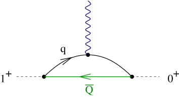
Figure 3.5: Physical interpretation of the gauge invariant axial-vector three-point function of a quark in terms of a weak light-quark transition in a heavy-light $\bar{Q}q$ meson.

The spectral representation of vector and axial-vector three-point functions is studied in some detail in the appendix 6.1. The main result is that in the limit that $y_{4}\gg z_{4}\gg x_{4}$ the ratio

$$\frac{{\rm Tr}[(\Pi^{a}_{AQQ})_{3}\gamma_{5}\gamma_{3}]}{{\rm Tr}[(\Pi^{a}_{VQQ})_{4}\gamma_{4}]}\to\frac{g_{A}}{g_{V}}$$ (3.55)

tends to the ratio of axial-vector and vector coupling constants, $g_{A}/g_{V}$. We therefore define the following Dirac traces

$$(\Pi^{a}_{VQQ})^{\mu\nu}(x,z,y) = {\rm Tr}[(\Pi^{a}_{VQQ})^{\mu}\gamma^{\nu}],$$ (3.56)

$$(\Pi^{a}_{AQQ})^{\mu\nu}(x,z,y) = {\rm Tr}[(\Pi^{a}_{AQQ})^{\mu}\gamma_{5}\gamma^{\nu}].$$ (3.57)

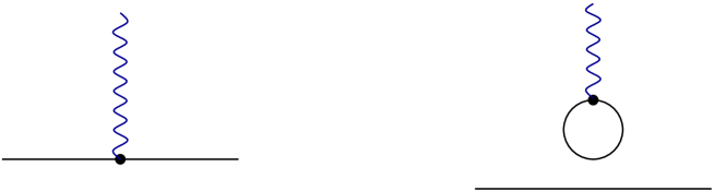
Figure 3.6: Quark line diagrams that contribute to the vector and axial-vector three-point function of a constituent quark. The solid lines denote quark propagators in a gluonic background field. The two diagrams show the connected and disconnected contribution.

As in the case of the two-point function the iso-triplet correlator only receives quark-line connected contributions, whereas the iso-singlet correlation function has a disconnected contribution, see Fig. 3.6. We find

$$(\Pi^{3}_{VQQ})^{\mu\nu}(x,z,y)=(P^{con}_{VQQ})^{\mu\nu}(x,z,y)=\langle{\rm Tr}[S(x,z)\gamma^{\mu}S(z,y)\gamma^{\nu}]\rangle$$ (3.58)

and

$$(\Pi^{0}_{VQQ})^{\mu\nu}(x,z,y)=(P^{con}_{VQQ})^{\mu\nu}(x,z,y)-2(P^{dis}_{VQQ})^{\mu\nu}(x,z,y)$$ (3.59)

with

$$(P^{dis}_{VQQ})^{\mu\nu}(x,z,y)=\langle{\rm Tr}[S(x,y)\gamma^{\mu}]{\rm Tr}[S(z,z)\gamma^{\nu}]\rangle,$$ (3.60)

as well as the analogous result for the axial-vector correlator.

In the following we compute the single instanton contribution to these correlation functions. We begin with the connected part. We again write the propagator in the field of the instanton as $S_{ZM}+S_{NZ}+S_{m}$ where $S_{ZM}$ is the zero-mode term, $S_{NZ}$ is the non-zero mode term, and $S_{m}$ is the mass correction. In the three-point correlation function we get contribution of the type $S_{NZ}S_{NZ}$, $S_{ZM}S_{m}$ and $S_{m}S_{ZM}$

$$(P^{con}_{A/VQQ})^{\mu\nu} = P_{NZNZ}^{\mu\nu}+c_{A/V}\left(P^{\mu\nu}_{ZMm}+P^{\mu\nu}_{mZM}\right)$$ (3.61)

$$= {\rm Tr}[S^{NZ}(x,z)\gamma^{\mu}S^{NZ}(z,y)\gamma^{\nu}]$$

$$+c_{A/V}{\rm Tr}[-\Psi_{0}(x)\Psi_{0}^{+}(z)\gamma^{\mu}(-\Delta_{\pm}(z,y)\gamma_{\pm}\gamma^{\nu}]$$

$$+c_{A/V}{\rm Tr}[(-\Delta_{\pm}(x,z)\gamma_{\pm})\gamma^{\mu}(-\Psi_{0}(z)\Psi_{0}^{+}(y))\gamma^{\nu}],$$

where the only difference between the vector and axial-vector case is the sign of ’ZMm’ and ’mZM’ terms. We have $c_{A/V}=\pm 1$ for vector (axial vector) current insertions. The detailed evaluation of the traces is quite tedious and we relegate the results to the appendix 6.2.

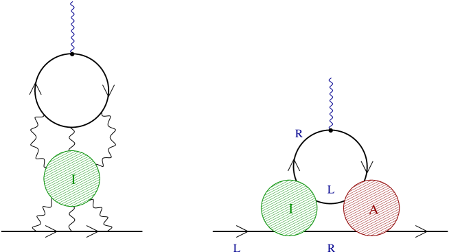
Figure 3.7: Instanton contributions to the disconnected axial-vector three-point correlation function of a quark. The left panel shows the single-instanton (non-zero mode) contribution. The right panel shows the instanton-anti-instanton (fermion zero mode) contribution.

Our main goal is the calculation of the disconnected correlation function, which is related to OZI violation. In the single instanton approximation only the axial-vector correlator receives a non-zero disconnected contribution

$$(P^{dis}_{AQQ})^{\mu\nu}={\rm Tr}[S(x,y)\gamma_{5}\gamma^{\nu}]{\rm Tr}[S(z,z)\gamma_{5}\gamma^{\mu}],$$ (3.62)

see Fig. 3.7. We observe that the second trace is the axial-vector current in the field of an instanton, see equ. (3.19). As for the first trace, it is easy to see that neither the zero mode part of the propagator nor the part of $S_{NZ}$ proportional to the free propagator can contribute. A straight-forward computation gives

$${\rm Tr}[S(x,y)\gamma_{5}\gamma^{\nu}]=\mp\frac{\rho^{2}}{\pi^{2}(x-y)^{2}x^{2}y^{2}}\frac{x^{\alpha}y^{\beta}(x-y)^{\sigma}}{\sqrt{(1+\frac{\rho^{2}}{x^{2}})(1+\frac{\rho^{2}}{y^{2}})}}\left(\frac{S^{\alpha\nu\sigma\beta}}{\rho^{2}+x^{2}}-\frac{S^{\alpha\sigma\nu\beta}}{\rho^{2}+y^{2}}\right).$$ (3.63)

Combined with equ. (3.19) we obtain

$$(P^{dis}_{AQQ})^{\mu\nu} = -\frac{2\rho^{4}z^{\mu}x^{\alpha}y^{\beta}(x-y)^{\sigma}}{\pi^{4}(x-y)^{2}x^{2}y^{2}(z^{2}+\rho^{2})^{3}}\frac{1}{\sqrt{(1+\frac{\rho^{2}}{x^{2}})(1+\frac{\rho^{2}}{y^{2}})}}$$ (3.64)

$$\hskip 8.5359pt\times\left(\frac{S^{\alpha\nu\sigma\beta}}{\rho^{2}+x^{2}}-\frac{S^{\alpha\sigma\nu\beta}}{\rho^{2}+y^{2}}\right),$$

which has to be multiplied by a factor 2 in order to take into account both instantons and anti-instantons.

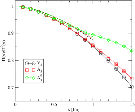
Figure 3.8: Axial and vector three-point functions of a quark as a function of the separation between the two quark sources. The correlation functions are normalized to free field behavior. The data points show results from numerical simulations of the instanton liquid and the dashed lines show the single instanton approximation.

Results for the vector three-point function $(\Pi_{VQQ}^{3})^{44}(\tau,\tau/2,0)$ and axial-vector three-point function $(\Pi_{AQQ}^{0,3})^{33}(\tau,\tau/2,0)$ are shown in Fig. 3.8. We observe that the vector and axial-vector correlation functions are very close to one another. We also note that the disconnected contribution adds to the connected part of the axial-vector three-point function. This can be understood from the short distance behavior of the correlation function. The disconnected part of the gauge invariant three-point function satisfies

$$\lim_{y,z\to x}\Big{\{}(\Pi_{AQQ}^{dis})^{33}(x,z,y)\Big{\}}=\lim_{x\to z}\Big{\{}{\rm Tr}[S(x,x)\gamma_{3}\gamma_{5}]{\rm Tr}[S(z,z)\gamma_{3}\gamma_{5}]\Big{\}}>0.$$ (3.65)

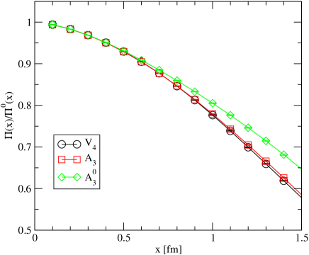
Figure 3.9: Axial and vector three-point functions of a quark as a function of the separation between the two quark sources. The data points show results from an unquenched instanton simulation.

This expression is exactly equal to the short distance term in the disconnected $f_{1}$ meson correlation function. The short distance behavior of the connected three-point function, on the other hand, is opposite in sign to the two-point function. This is related to the fact that the two-point function involves one propagator in the forward direction and one in the backward direction, whereas the three-point function involves two forward propagating quarks. A similar connection between the interaction in the $f_{1}$ meson channel and the flavor singlet coupling of a constituent quark was found in a Nambu-Jona-Lasinio model [82, 83]. It was observed, in particular, that an attractive coupling in the $f_{1}$ channel is needed in order to suppress the flavor singlet $(g_{A}^{0})_{Q}$.

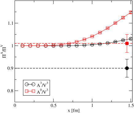
Figure 3.10: Ratio of axial-vector to vector correlation functions of a constituent quark calculated in the instanton liquid model. The open points show point-to-point correlation functions while the solid point is the zero momentum (point-to-plane) limit. The figure shows the iso-vector and iso-singlet correlation functions.

The same general arguments apply to the short distance contribution from instanton-anti-instanton pairs. At long distance, on the other hand, we expect that IA pairs reduce the flavor singlet axial current correlation function. The idea can be understood from Fig. 3.7, see [58, 84, 85]. In an IA transition a left-handed valence up quark emits a right handed down quark which acts to shield its axial charge. We have studied this problem numerically, see Figs. 3.8-3.10. We find that in quenched simulations the flavor singlet axial three-point function is significantly enhanced. This effect is analogous to what we observed in the $f_{1}$ channel and disappears in unquenched simulations. We have also studied the axial three-point function at zero three-momentum $\vec{q}=0$. This correlation function is directly related to the coupling constant, see App. 6.1. We find that the iso-vector coupling is smaller than one, $(g_{A}^{3})_{Q}\simeq 0.9$, in agreement with Weinberg’s idea. The flavor singlet coupling, on the other hand, is close to one. We observe no suppression of the singlet charge of a constituent quark. We have also checked that this result remains unchanged in unquenched simulations.

3.5 Axial Structure of the Nucleon

In this section we shall study the axial charge of the nucleon in the instanton model. We consider the same correlation functions as in the previous section, but with the quark field replaced by a nucleon current. The vector three-point function is given by

$$(\Pi^{a}_{VNN})^{\alpha\beta}_{\mu}(x,y)=\langle\eta^{\alpha}(0)V^{a}_{\mu}(y)\bar{\eta}^{\beta}(x)\rangle.$$ (3.66)

Here, $\eta^{\alpha}$ is a current with the quantum numbers of the nucleon. Three-quark currents with the nucleon quantum numbers were introduced by Ioffe [86]. He showed that there are two independent currents with no derivatives and the minimum number of quark fields that have positive parity and spin $1/2$. In the case of the proton, the two currents are

$$\eta_{1}=\epsilon_{abc}(u^{a}C\gamma_{\mu}u^{b})\gamma_{5}\gamma_{\mu}d^{c},\hskip 28.45274pt\eta_{2}=\epsilon_{abc}(u^{a}C\sigma_{\mu\nu}u^{b})\gamma_{5}\sigma_{\mu\nu}d^{c}.$$ (3.67)

It is sometimes useful to rewrite these currents in terms of scalar and pseudo-scalar diquark currents. We find

$$\eta_{1} = 2\left\{\epsilon_{abc}(u^{a}Cd^{b})\gamma_{5}u^{c}-\epsilon_{abc}(u^{a}C\gamma_{5}d^{b})u^{c}\right\},$$ (3.68)

$$\eta_{2} = 4\left\{\epsilon_{abc}(u^{a}Cd^{b})\gamma_{5}u^{c}+\epsilon_{abc}(u^{a}C\gamma_{5}d^{b})u^{c}\right\}.$$ (3.69)

Instantons induce a strongly attractive interaction in the scalar diquark channel $\epsilon^{abc}(u^{b}C\gamma_{5}d^{c})$ [69, 87]. As a consequence, the nucleon mainly couples to the scalar diquark component of the Ioffe currents $\eta_{1,2}$. This phenomenon was also observed on the lattice [88]. This result is suggestive of a model of the spin structure that is quite different from the naive quark model. In this picture the nucleon consists of a tightly bound scalar-isoscalar diquark, loosely coupled to the third quark [89]. The quark-diquark model suggests that the spin and isospin of the nucleon are mostly carried by a single constituent quark, and that $g_{A}^{N}\simeq g_{A}^{Q}$.

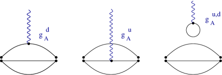
Figure 3.11: Quark line diagrams that contribute to the axial-vector three-point function of the proton. The solid lines denote quark propagators in a gluonic background field. The lines are connected in the same way that the Dirac indices of the propagators are contracted. The iso-vector and iso-singlet correlation functions correspond to $g_{A}^{u}=-g_{A}^{d}=1$ and $g_{A}^{u}=g_{A}^{d}=1$, respectively. The disconnected diagram only contributes to the iso-scalar three-point function.

Nucleon correlation functions are defined by $\Pi^{N}_{\alpha\beta}(x)=\langle\eta_{\alpha}(0)\bar{\eta}_{\beta}(x)\rangle$, where $\alpha,\beta$ are Dirac indices. The correlation function of the first Ioffe current is

$$\Pi_{\alpha\beta}(x)=2\epsilon_{abc}\epsilon_{a^{\prime}b^{\prime}c^{\prime}}\,\langle\left(\gamma_{\mu}\gamma_{5}S_{d}^{cc^{\prime}}(0,x)\gamma_{\nu}\gamma_{5}\right)_{\alpha\beta}\,{\rm Tr}\left[\gamma_{\mu}S_{u}^{aa^{\prime}}(0,x)\gamma_{\nu}C(S_{u}^{bb^{\prime}}(0,x))^{T}C\right]\rangle.$$ (3.70)

The vector and axial-vector three-point functions can be constructed in terms of vector and axial-vector insertions into the quark propagator,

$$(\Gamma^{V}_{\mu})_{f}^{aa^{\prime}}(x,y) = S_{f}^{ab}(0,y)\gamma_{\mu}S_{f}^{ba^{\prime}}(y,x),$$ (3.71)

$$(\Gamma^{A}_{\mu})_{f}^{aa^{\prime}}(x,y) = S_{f}^{ab}(0,y)\gamma_{\mu}\gamma_{5}S_{f}^{ba^{\prime}}(y,x).$$ (3.72)

The three-point function is given by all possible substitutions of equ. (3.71) and (3.72) into the two-point function. We have

$$(\Pi^{a}_{VNN})^{\alpha\beta}_{\mu}(x,y)=2\epsilon_{abc}\epsilon_{a^{\prime}b^{\prime}c^{\prime}}\times$$

$$\times\langle\Bigg{\{} g_{V}^{d}\left(\gamma_{\rho}\gamma_{5}(\Gamma^{V}_{\mu})_{d}^{cc^{\prime}}(x,y)\gamma_{\sigma}\gamma_{5}\right)_{\alpha\beta} {\rm Tr}\left[\gamma_{\rho}S_{u}^{aa^{\prime}}(0,x)\gamma_{\sigma}C(S_{u}^{bb^{\prime}}(0,x))^{T}C\right]$$

$$+ 2g_{V}^{u}\left(\gamma_{\rho}\gamma_{5}S_{d}^{cc^{\prime}}(0,x)\gamma_{\sigma}\gamma_{5}\right)_{\alpha\beta} {\rm Tr}\left[\gamma_{\rho}(\Gamma^{V}_{\mu})_{u}^{aa^{\prime}}(x,y)\gamma_{\sigma}C(S_{u}^{bb^{\prime}}(0,x))^{T}C\right]$$

$$- \left(\gamma_{\rho}\gamma_{5}S_{d}^{cc^{\prime}}(0,x)\gamma_{\sigma}\gamma_{5}\right)_{\alpha\beta} {\rm Tr}\left[\gamma_{\rho}S_{u}^{aa^{\prime}}(0,x)\gamma_{\sigma}C(S_{u}^{bb^{\prime}}(0,x))^{T}C\right]$$ (3.73)

$$\times{\rm Tr}\left[g_{V}^{u}\gamma_{\mu}S_{u}^{dd}(y,y)+g_{V}^{d}\gamma_{\mu}S_{d}^{dd}(y,y)\right]\Bigg{\}}\rangle,$$

where the first term is the vector insertion into the $d$ quark propagator in the proton, the second term is the insertion into the $uu$ diquark, and the third term is the disconnected contribution, see Fig. 3.11. The vector charges of the quarks are denoted by $g_{V}^{f}$. In the case of the iso-vector three-point function we have $g_{V}^{u}=1$, $g_{V}^{d}=-1$ and in the iso-scalar case $g_{V}^{u}=g_{V}^{d}=1$.

Vector and axial-vector three-point functions of the nucleon are shown in Figs. 3.12 and 3.13. In order to verify that the correlation functions are dominated by the nucleon pole contribution we have compared our results to the spectral representation discussed in the appendix 6.1, see Fig. 3.12. The nucleon coupling constant was determined from the nucleon two-point function. The figure shows that we can describe the three-point functions using the phenomenological values of the vector and axial-vector coupling constants. We have also checked that the ratio of axial-vector and vector current three-point functions is independent of the nucleon interpolating field for $x>1$ fm. The only exception is a pure pseudo-scalar diquark current, which has essentially no overlap with the nucleon wave function.

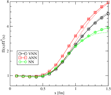
Figure 3.12: Vector, axial-vector three-point functions of the nucleon and nucleon two-point function calculated in the instanton liquid model. All correlation functions are normalized to free field behavior. The results are compared to a simple pole fit of the type discussed in the appendix.

The main result is that the iso-vector axial-vector correlation function is larger than the vector correlator. The corresponding ratio is shown in Fig. 3.13, together with the ratio of $\vec{q}=0$ correlation functions. We find that the iso-vector axial coupling constant is $g_{A}^{3}=1.28$, in good agreement with the experimental value. We also observe that the ratio of point-to-point correlation functions is larger than this value. As explained in the appendix, this shows that the axial radius of the nucleon is smaller than the vector radius. Taking into account only the connected part of the correlation function we find a singlet coupling $g_{A}^{0}=0.79$. The disconnected part is very small, $g_{A}^{0}(dis)=-(0.02\pm 0.02)$. Assuming that $\Delta s\simeq\Delta u(dis)=\Delta d(dis)$ this implies that the OZI violating difference $g_{A}^{8}-g_{A}^{0}$ is small. This result does not change in going from the quenched approximation to full QCD.

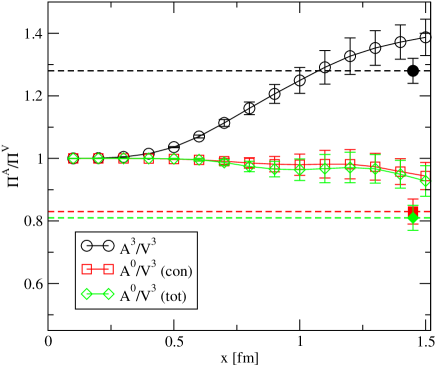
Figure 3.13: Ratio of axial-vector to vector correlation functions of the nucleon calculated in the instanton liquid model. The open points show point-to-point correlation functions while the solid point is the zero momentum (point-to-plane) limit. The figure shows the iso-vector, connected iso-singlet, and full iso-singlet axial-vector correlation functions.

We have also studied the dependence of the results on the average instanton size, see Fig. 3.14. We observe that there is a slight decrease in the iso-singlet coupling and a small increase in the iso-vector coupling as the instanton size is decreased. What is surprising is that the disconnected term changes sign between $\rho=0.3$ fm and $\rho=0.35$ fm. The small value $g_{A}^{0}(dis)=-(0.02\pm 0.02)$ obtained above is related to the fact that the phenomenological value of the instanton size is close to the value where $g_{A}^{0}(dis)$ changes sign. However, even for $\rho$ as small as 0.2 fm the disconnected contribution to the axial coupling $g_{A}^{0}(dis)=-(0.05\pm 0.02)$ is smaller in magnitude than phenomenology requires.

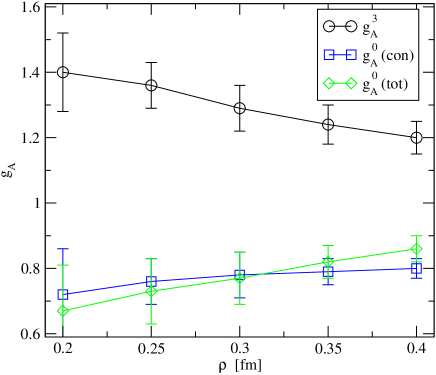
Figure 3.14: Axial coupling constants of the nucleon as a function of the instanton size $\rho$ with the instanton density fixed at $(N/V)=1\,{\rm fm}^{-4}$. We show the iso-vector, connected iso-singlet, and full iso-singlet axial coupling constant.

3.6 Conclusions

The main issue raised by the EMC measurement of the flavor singlet axial coupling is not so much why $g_{A}^{0}$ is much smaller than one - except for the naive quark model there is no particular reason to expect $g_{A}^{0}$ to be close to one - but why the OZI violating observable $g_{A}^{0}-g_{A}^{8}$ is large. Motivated by this question we have studied the contribution of instantons to OZI violation in the axial-vector channel. We considered the $f_{1}-a_{1}$ meson splitting, the flavor singlet and triplet axial coupling of a constituent quark, and the axial coupling constant of the nucleon. We found that instantons provide a short distance contribution which is repulsive in the $f_{1}$ meson channel and adds to the gauge invariant flavor singlet three-point function of a constituent quark. We showed that the sign of this term is fixed by positivity arguments.

We computed the axial coupling constants of the constituent quark and the nucleon using numerical simulations of the instanton liquid. We find that the iso-vector axial coupling constant of a constituent quark is $(g_{A}^{3})_{Q}=0.9$ and that of a nucleon is $g_{A}^{3}=1.28$, in good agreement with experiment. The result is also in qualitative agreement with the constituent quark model relation $g_{A}^{3}=5/3\cdot(g_{A}^{3})_{Q}$. The flavor singlet coupling of quark is close to one, while that of a nucleon is suppressed, $g_{A}^{0}=0.77$. However, this value is still significantly larger than the experimental value $g_{A}^{0}=(0.28-0.41)$. In addition to that, we find very little OZI violation, $\Delta s\simeq\Delta u(dis)\simeq-0.01$. We observed, however, that larger values of the disconnected contribution can be obtained if the average instanton size is smaller than the phenomenological value of $\rho\simeq 1/3$ fm.

There are many questions that remain to be addressed. In order to understand what is missing in our calculation it would clearly be useful to perform a systematic study of OZI violation in the axial-vector channel on the lattice. The main question is whether the small value of $g_{A}^{0}$ is a property of the nucleon, or whether large OZI violation is also seen in other channels. A study of the connected contributions to the axial coupling constant in cooled as well as quenched quantum QCD configurations was performed in [90]. These authors find $g_{A}^{0}(con)=\Delta u(con)+\Delta d(con)\simeq 0.6$ in both cooled and full configurations. The disconnected term was computed by Dong et al. [91]. They find $\Delta u(dis)+\Delta d(dis)\simeq-0.24$.

In the context of the instanton model it is important to study whether the results for $g_{A}^{0}$ obtained from the axial-vector current three-point function are consistent with calculations of $g_{A}^{0}$ based on the matrix element of the topological charge density $G\tilde{G}$ [92, 93, 94, 95]. It would also be useful to further clarify the connection of the instanton liquid model to soliton models of the nucleon [96]. In soliton models the spin of the nucleon is mainly due to the collective rotation of the pion cloud, and a small value for $g_{A}^{0}$ is natural [97, 98]. The natural parameter that can be used in order to study whether this picture is applicable is the number of colors, $N_{c}$. Unfortunately, a direct calculations of nucleon properties for $N_{c}>3$ would be quite involved. Finally it would be useful to study axial form factors of the nucleon. It would be interesting to see whether there is a significant difference between the iso-vector and iso-singlet axial radius of the nucleon. A similar study of the vector form factors was recently presented in [99].

Chapter 4 Group integration

4.1 General remarks

Group integration became an important tool in physics with the development of lattice gauge theories[101]. Since then it enjoyed more attention in other areas as well, like instantons [102, 103] or random matrix theory, e.g.[104]. In this chapter we elaborate on an idea of Michael Creutz and present an algorithm for computing integrals over elements of a compact group.

A lot of progress has been made in the direction of solving the generating functional

$$Z(J,J^{\dagger})=\int\!\!du\;\exp\{J^{\dagger}u+u^{\dagger}J\}\>\>,$$ (4.1)

which enables one to express any other integral of a general function $f(u,u^{\dagger})$ as:

$$\int\!\!du\;f(u,u^{\dagger})=\left.f(\delta_{J^{\dagger}},\delta_{J})\;\;Z(J,J^{\dagger})\right|_{J,J^{\dagger}=0}.$$ (4.2)

Different methods have been used to compute (4.1). Direct integration over parametrized $SU(2)$ and $SU(3)$ was given in [105], and polar decomposition of $U(N)$ and integration over angular variables in [106]. Another approach was to construct and solve a partial differential equation which $Z(J,J^{\dagger})$ satisfies due to its invariance w.r.t. left and right actions of the group[107, 108]. The author of [109] expanded $Z(J,J^{\dagger})$ in powers of invariants and computed numerically the coefficients up to some order using again a differential equation. Character expansion (for recent work see [111]) proved to be a powerful method, used for $U(N)$ in [110]. More recently[104] a $\frac{1}{N}$ expansion of integrals over monomials in $U(N)$ and $O(N)$ matrix elements was developed, with the leading and next-to-leading order terms computed using a standard integral over $\mathbf{C}^{N^{2}}$ with a modified Gaussian measure.

The method we propose lacks the elegance of character expansion of generating functional. Its simplicity, however, makes it a handy tool for evaluating group integrals over any compact group and any representation. Moreover, it is easily implementable as a computer algorithm once the group invariants are known. The same idea may also be applied to evaluating integrals of tensorial structure over any manifold with a measure possessing some kind of symmetry.

The flow of ideas has the following structure: in section 4.2 we introduce the main properties of Haar measure. We state the algorithm in section 4.3 and exemplify it on fundamental and adjoint representations of $SU(N)$ in section 4.4 and 4.5 respectively.

4.2 Properties of Haar measure

The algorithm being proposed relies heavily on the properties of the Haar measure :

For any compact group there exists a unique left-right invariant measure, normalized to unity, such that:

$$\int\!\!du = 1$$ (4.3)

$$\int\!\!du\;f(gu) = \int\!\!du\;f(ug)=\int\!\!du\;f(u)$$ (4.4)

$$\int\!\!du\;f(u) = \int\!\!du\;f(u^{-1})\>\>,$$ (4.5)

where $u,g$ are elements of the group and $du$ is the Haar measure.

The left-right invariance of the measure is the analog of translational invariance of the $\mathbf{R}^{n}$ integral and for finite groups represents the invariability of the number of elements w.r.t. multiplication by a fixed element of the group. The examples of group measure [101]:

for $U(1)=\{e^{i\phi}\>|\>-\pi<\phi\leq\pi\}$:

$$\int\!\!du\;f(u)=\frac{1}{2\pi}\int_{-\pi}^{\pi}\!\!d\phi\;f(e^{i\phi})$$ (4.6)

for $SU(2)=\{a_{0}+i\vec{a}\cdot\vec{\tau}\>|\>a_{0}^{2}+\vec{a}^{2}=1\}$:

$$\int\!\!du\;f(u)=\frac{1}{\pi^{2}}\int\!\!d^{4}a\>\delta(a^{2}-1)\>f(u(a))$$ (4.7)

4.3 The algorithm for group integration

We will present here the main idea, mentioned before in [108] but, to our knowledge, never carried out completely.

For the purpose of integration we will not need an exact expression for the measure, like (4.6),(4.7). We will only use the general properties of the Haar measure, making the algorithm applicable to any compact group.

We are interested in the most general integral of a monomial in group elements:

$$I_{\underbrace{i_{1}\ldots i_{n}}_{{}^{\prime}left^{\prime}},\underbrace{j_{1}\ldots j_{n}}_{{}^{\prime}right^{\prime}\;indices}}^{\overbrace{l_{1}\ldots l_{m}}\>,\>\overbrace{k_{1}\ldots k_{m}}}=\int\!\!du\>u_{i_{1}j_{1}}\ldots u_{i_{n}\ldots j_{n}}\>\bar{u}^{k_{1}l_{1}}\ldots\bar{u}^{k_{m}l_{m}}\>\>,$$ (4.8)

where $\bar{u}$ represents $u^{\dagger}$ for SU(N) or $u^{+}$ for SO(N) or $u^{-1}$ for a general compact group.

In order to exemplify the idea, we will consider first the simple example of

$$I_{i,j}^{l,k}=\int\!\!du\>u_{ij}\>\bar{u}^{kl}\>\>.$$ (4.9)

The right invariance (4.4) implies:

$$I_{i,j}^{l,k}=\bar{g}_{kk^{\prime}}\>I_{i,j^{\prime}}^{l,k^{\prime}}\>g_{j^{\prime}j}\>\>.$$ (4.10)

This shows that $I_{i,j}^{l,k}$ has to be an invariant of the group in ’right’ indices $j,k$. The same argument with left invariance of the measure compels $I_{i,j}^{l,k}$ to be separately an invariant in ’left’ indices $i,l$ as well. There is only one second rank invariant tensor with upper and lower index for SU(N): $\delta_{i}^{l}$. Therefore, the integral (4.9) has to be of the form:

$$I_{i,j}^{l,k}=a_{1}\>\delta_{i}^{l}\>\delta_{j}^{k}\>\>.$$

The constant $a_{1}$ is found easily by contracting with $\delta_{j}^{k}$ and using $u_{ij}\bar{u}^{jl}=\delta_{i}^{l}$ and the unit normalization (4.3):

$$\delta_{i}^{l}=I_{i,j}^{l,j}=a_{1}\>N\>\delta_{i}^{l}\>\>.$$

So the integral then is:

$$I_{i,j}^{l,k}=\int\!\!du\>u_{ij}\>\bar{u}^{kl}=\frac{1}{N}\>\delta_{i}^{l}\>\delta_{j}^{k}\>\>,$$ (4.11)

which is nothing else but the orthogonality relation for fundamental representation. The non-existence of one-index invariant leads directly to

$$I_{i,j}=\int\!\!du\>u_{ij}=0\>\>.$$ (4.12)

The same steps as in the above examples can be followed for any integral of the type (4.8). Let us summarize them in the form of the following algorithm:

• Generate all the independent invariant tensors with the index structure of (4.8). The result of integration will be take the form:

  $$\sum_{all\>invariants}const\times(left\>\>indices\>\>invariant)\times(right\>\>indices\>\>invariant).$$

• Use index pairs exchange symmetry(e.g. $i_{1}j_{1}\leftrightarrow i_{2}j_{2}$) to identify the tensors with the same numerical coefficients.

• Compute the independent coefficients by multiplying (4.8) with the corresponding invariant tensors (e.g. contracting indices with $\delta$ tensor).

Throughout the this work we deal with SU(N). However, the same philosophy is applicable to any compact group.

4.4 Integration over fundamental representation of SU(N)

The invariant tensors depend on the group (e.g. vary with N in SU(N)) as well as representation. For fundamental representation of SU(N) we have two basic invariants, out of which the rest is constructed: $\delta_{i}^{l}$ and $\epsilon^{i_{1}\ldots i_{N}}$. The invariance can be seen easily from the unitarity and unimodularity.

The result of a particular integral will depend on N, e.g.

$$\int\!\!du\>u_{i_{1}j_{1}}\>u_{i_{2}j_{2}}=\left\{\begin{array}[]{ll}\frac{1}{2}\epsilon_{i_{1}i_{2}}\epsilon_{j_{1}j_{2}}&\mbox{for $SU(2)$}\\ 0&\mbox{for $SU(N>2)$}\end{array}\right.\>\>.$$ (4.13)

Despite of having different invariants for different N, there are many cases the result has the same form, but coefficients depend on N. An example is the integral with the same number of $u$ and $\bar{u}$’s, schematically $I_{n}\equiv\int\!\!du(u\>\bar{u})^{n}$,on which we will focus in this paragraph.

Let us then follow the proposed algorithm and compute $I_{n}$. First we generate all left-right invariant terms. Using symmetries of the measure we identify the terms with the same numeric coefficients. Finally we multiply both sides with the very same set of invariants and solve the obtained system of linear equations for the unknown coefficients.

So what are the possible invariants we can construct? The building blocks are Kronecker’s $\delta$ and $\epsilon$ tensors.

First of all, there are $(n!)^{2}$ terms of the form

$$(\underbrace{\delta\times\ldots\times\delta}_{n\times left\>indices})\times(\underbrace{\delta\times\ldots\times\delta}_{n\times right\>indices})\>\>,$$ (4.14)

i.e. a $\delta$ for each up-down pair both in left and right indices.

Then, for $n>N$ we can use $\epsilon_{i_{1}\ldots i_{N}}$ or $\epsilon^{l_{1}\ldots l_{N}}$ to form terms like

$$(\underbrace{\delta\times\ldots\delta}_{n-N}\times\epsilon_{lower\>indices}\times\epsilon^{upper\>indices})_{left}\times(\ldots)_{right}\>\>.$$ (4.15)

Notice that $\epsilon$ tensors must come in pairs, both with upper and lower indices, left or right(or both). The reason is obvious: $\delta$’s require both an upper and a lower index; if an $\epsilon$ with lower indices is used, then the only invariant left for upper extra indices is another $\epsilon$. One could thus have pairs of $\epsilon$ in left and right indices, having different structure for different N. Fortunately, this is not the case, as products of $\epsilon$’s can be expanded in products of $\delta$’s.

The important observation is, that any pair of $\epsilon$’s in upper and lower indices can be written as a completely antisymmetric sum of products of Kronecker $\delta$ tensors:

$$\epsilon_{i_{1}i_{2}\ldots i_{n}}\epsilon^{l_{1}l_{2}\ldots l_{n}}=\sum_{permutations\>P}(-1)^{P}\delta_{i_{1}}^{P(l_{1})}\ldots\delta_{i_{n}}^{P(l_{n})}\>\>.$$ (4.16)

Therefore, independently on N, the final result will only contain products of $\delta$’s, it will be of the form of (4.14).

Having noticed this, we only need to generate all the possible ($\delta)^{n}\times(\delta)^{n}$ combinations, identify common coefficients and compute them.(the actual values of coefficients will depend on N).

We will present the calculation up to $n=3$, for the higher order integrals one would use a computer program to generate terms and compute the coefficients.

4.4.1 Case n=2

We will treat the integral

$$I_{i_{1}i_{2},j_{1}j_{2}}^{l_{1}l_{2},k_{1}k_{2}}=\int\!\!du\>u_{i_{1}j_{1}}\>\bar{u}^{k_{1}l_{1}}\>u_{i_{2}j_{2}}\>\bar{u}^{k_{2}l_{2}}$$ (4.17)

in some detail in order to unveil the ideas that are useful in the more involving case of higher n.

The integral will contain $(2!)\times(2!)$ terms:

$$\raisebox{-21.33955pt}{ \psfig{width=341.43306pt,height=42.67912pt} },$$ (4.18)

where we represent $\delta$ by a line joining the indices. Each line has to join an upper left(right) index with a lower left(right) index. No connections between left and right indices are allowed. The indices in the above graphs have always the same position as in the first parenthesis of (4.18)

The $(i_{1}j_{1})\leftrightarrow(i_{2}j_{2})$ and $(k_{1}l_{1})\leftrightarrow(k_{2}l_{2})$ symmetry of (4.17) allows us to identify the equal coefficients among $b_{1}\ldots b_{4}$. Under $(i_{1}j_{1})\leftrightarrow(i_{2}j_{2})$ the diagrams (1 and 4) as well as (2 and 3) interchange. Therefore $b_{1}=b_{4}$ and $b_{2}=b_{3}$.

It is easy to identify the diagrams that have the same coefficients by the topology of diagrams. Take pairs of 1 left and 1 right index, e.g. lower $(i_{1}j_{1}),(i_{2}j_{2})$ or upper $(l_{1}k_{1}),(l_{2}k_{2})$. What matters is how many of these pairs of indices are interconnected: in $b_{1}$ and $b_{4}$ terms one only has (1 upper pair - 1 lower pair) $\delta$ connections. These two diagrams are pair-exchange equivalent. The $b_{2}$ diagram is topologically different: there is a (2 upper pairs - 2 lower pairs) $\delta$-interconnection: both pairs of upper indices (lk) are connected to both pairs of lower (ij) indices. This diagram is pair-exchange equivalent to $b_{3}$ and falls in the same topological set of diagrams. This easy way to identify diagrams with the same coefficients will prove very useful in calculating integrals with higher n.

Computing the coefficients is straight-forward: contract with ’right’ $\delta_{j_{1}}^{k_{1}}$ to get on one hand, from (4.11):

$$\frac{1}{N}\delta_{i_{1}}^{l_{1}}\delta_{i_{2}}^{l_{2}}\delta_{j_{2}}^{k_{2}}$$

and, on the other hand (4.18):

$$(N\>b_{1}+b_{2})\delta_{i_{1}}^{l_{1}}\delta_{i_{2}}^{l_{2}}\delta_{j_{2}}^{k_{2}}+(N\>b_{2}+b_{1})\delta_{i_{1}}^{l_{2}}\delta_{i_{2}}^{l_{1}}\delta_{j_{2}}^{k_{2}}\>\>.$$

Matching the two sides we get the coefficients. The result then is:

$$\begin{split}&I_{i_{1}i_{2},j_{1}j_{2}}^{l_{1}l_{2},k_{1}k_{2}}=\int\!\!du\>u_{i_{1}j_{1}}\>\bar{u}_{k_{1}l_{1}}\>u_{i_{2}j_{2}}\>\bar{u}_{k_{2}l_{2}}=\\ &=\frac{1}{N^{2}-1}\left[\raisebox{-11.38092pt}{ \psfig{width=85.35826pt,height=28.45274pt} }\right]-\frac{1}{N(N^{2}-1)}\left[\raisebox{-11.38092pt}{ \psfig{width=85.35826pt,height=28.45274pt} }\right]\\ &=\frac{1}{N^{2}-1}[\delta_{i_{1}}^{l_{1}}\delta_{j_{1}}^{k_{1}}\delta_{i_{2}}^{l_{2}}\delta_{j_{2}}^{k_{2}}+\delta_{i_{1}}^{l_{2}}\delta_{j_{1}}^{k_{2}}\delta_{i_{2}}^{l_{1}}\delta_{j_{2}}^{k_{1}}]-\frac{1}{N(N^{2}-1)}[\delta_{i_{1}}^{l_{1}}\delta_{j_{1}}^{k_{2}}\delta_{i_{2}}^{l_{2}}\delta_{j_{2}}^{k_{1}}+\delta_{i_{1}}^{l_{2}}\delta_{j_{1}}^{k_{1}}\delta_{i_{2}}^{l_{1}}\delta_{j_{2}}^{k_{2}}]\\ \end{split}$$ (4.19)

4.4.2 Case n=3

The number of terms in

$$I_{i_{1}i_{2}i_{3},j_{1}j_{2}j_{3}}^{l_{1}l_{2}l_{3},k_{1}k_{2}k_{3}}=\int\!\!du\>u_{i_{1}j_{1}}\>\bar{u}^{k_{1}l_{1}}\>u_{i_{2}j_{2}}\>\bar{u}^{k_{2}l_{2}}\>u_{i_{3}j_{3}}\>\bar{u}^{k_{3}l_{3}}$$ (4.20)

increases to $(3!)\times(3!)=36$. They will be grouped in 3 topologically different classes having the same coefficients in the front:

• 6 terms of type (1-1,1-1,1-1), like e.g.

  

  linking 1 pair of upper to 1 pair of lower indices.

• 18 terms of type (2-2, 1-1) having 2 pairs of lower and 2 pairs of upper indices interconnected in addition to one upper to one lower pair $\delta$ connection. Examples of diagrams from this category:

  

• 12 terms of type(3-3) having all 3 pairs of upper indices and 3 pairs of lower indices interconnected, e.g. diagrams:

  

The coefficients can be found in a similar way to the case of $n=2$. The result is:

$$\int\!\!du\>u_{i_{1}j_{1}}\>\bar{u}^{k_{1}l_{1}}\>u_{i_{2}j_{2}}\>\bar{u}^{k_{2}l_{2}}\>u_{i_{3}j_{3}}\>\bar{u}^{k_{3}l_{3}}=$$ (4.21)

$$c_{1}\left[\raisebox{-17.07182pt}{ \psfig{width=113.81102pt,height=35.56593pt} }+\ldots altogether\;\;6\;\;terms\right]+$$

$$+ c_{2}\left[\raisebox{-17.07182pt}{ \psfig{width=113.81102pt,height=35.56593pt} }+\ldots altogether\;\;18\;\;terms\right]+$$

$$+ c_{3}\left[\raisebox{-17.07182pt}{ \psfig{width=113.81102pt,height=35.56593pt} }+\ldots altogether\;\;12\;\;terms\right],$$

where different terms in $\ldots$ are generated by interchanges of $(lk)$ pairs or $(ij)$ pairs, and have the same topology as the first term in parenthesis.

For $SU(N\geq 3)$ the coefficients are:

$$c_{1} = \frac{(N^{2}-2)}{N(N^{2}-1)(N^{2}-4)}$$

$$c_{2} = -\frac{1}{(N^{2}-1)(N^{2}-4)}$$

$$c_{3} = \frac{2}{N(N^{2}-1)(N^{2}-4)}$$ (4.22)

An important requirement is, that the invariant tensors are independent. The 3! terms of type $\delta_{i_{1}}^{l_{1}}\delta_{i_{2}}^{l_{2}}\delta_{j_{2}}^{k_{2}}$ and permutations are indeed independent for $SU(N),N\geq 3$. However, for $N=2$ there are ’too many’ indices and only 2 possible values for each index. This leads to the following relationship:

$$0=\epsilon_{i_{1}i_{2}i_{3}}\epsilon^{l_{1}l_{2}l_{3}}=\left[\raisebox{-12.80365pt}{ \psfig{width=256.0748pt,height=28.45274pt} }\right].$$ (4.23)

In this case of having dependent tensors one can follow the same strategy up to one point: after contracting the indices in order to figure out the coefficients, one has to express everything in terms of a basis of independent tensors, and only then compare the coefficients. For SU(2) this leads to the same form of result (4.21) with the parameter-dependent coefficients:

$$c_{1} = t+\frac{1}{6}$$

$$c_{2} = -t-\frac{1}{24}$$

$$c_{3} = t$$ (4.24)

The parameter t cancels if one goes to the basis of 5 independent $\delta\delta\delta$ tensors so we can as well set it to zero.

For higher $n=4,5\ldots$ one has to take this subtlety into account also for $SU(3),SU(4)\ldots$ The same idea will prove useful in the next paragraph, when we treat the integral over adjoint representation.

4.5 The integral over adjoint representation of SU(N)

In a number of cases one encounters integrals of type

$$I_{\underbrace{a_{1}a_{2}\ldots a_{n}}_{left},\underbrace{b_{1}b_{2}\ldots b_{n}}_{right}}=\int\!\!du\>R^{a_{1}b_{1}}R^{a_{2}b_{2}}\ldots R^{a_{n}b_{n}}\>\>,$$ (4.25)

where

$$R^{ab}=\frac{1}{2}Tr(\lambda^{b}u\lambda^{a}\bar{u})$$

is the adjoint representation of $SU(N)$ satisfying $R^{ab}\lambda^{b}=u\lambda^{a}\bar{u}$, with $\lambda^{a}$ the generators of SU(N) normalized to $Tr(\lambda^{a}\lambda^{b})=2\delta_{b}^{a}$.

To solve this integral, one can straight-forwardly integrate over u’s and then contract the result with $\lambda$’s and perform the trace. For example:

$$\int\!\!du\>R^{ab} = \frac{1}{2}\lambda^{b}_{li}\lambda^{a}_{jk}\int\!\!du\>u_{ij}\>\bar{u}_{kl}$$ (4.26)

$$= \frac{1}{2}\lambda^{b}_{li}\lambda^{a}_{jk}\frac{1}{N}\delta_{jk}\delta_{il}=\frac{1}{2N}Tr\lambda^{b}\>Tr\lambda^{a}=0\>\>.$$

For higher n the number of terms of $\int\!\!du\>(u\bar{u})^{n}$ grows as $(n!)^{2}$ and the evaluation of the integral, although straight-forward, becomes tedious. For this reason, we present here a more manageable way of computation, based on the above algorithm.

First of all, let’s note some properties of $R^{ab}$ matrices:

• $R^{ab}$ is the adjoint representation of $SU(N)$ group:

  $$R^{ab}_{uu^{\prime}}=R^{ac}_{u^{\prime}}\>R^{cb}_{u}$$ (4.27)

• The matrices form a subgroup of $SO(N^{2}-1)$:

  $$R^{ab}R^{cb}=R^{ab}(R^{+})^{bc}=\delta^{ac}$$ (4.28)

• Under the left-right action of the group, it rotates as follows:

  $$R^{ab}\stackrel{{\scriptstyle u\rightarrow g\>u\>h}}{{\longrightarrow}}\tilde{R}^{ab}=R^{bc}_{g^{-1}}\>R^{ad}_{h}\>R^{dc}=R^{ad}_{h}\>R^{dc}\>R^{cb}_{g}$$ (4.29)

The main idea of the algorithm applies here as well: the left-right invariance of the measure in (4.25) implies that

$$I_{a_{1}\ldots a_{n},b_{1}\ldots b_{n}}=R^{a_{1}a_{1}^{\prime}}_{h}\ldots R^{a_{n}a_{n}^{\prime}}_{h}R^{b_{1}b_{1}^{\prime}}_{g^{-1}}\ldots R^{b_{n}b_{n}^{\prime}}_{g^{-1}}\times I_{a_{1}^{\prime}\ldots a_{n}^{\prime},b_{1}^{\prime}\ldots b_{n}^{\prime}}\>\>.$$ (4.30)

In other words, $I_{a_{1}\ldots a_{n},b_{1}\ldots b_{n}}$ has to be of the form

$$\sum_{all\>invariants}const\times(invariant\>\>in\>\>left\>\>indices)\times(invariant\>\>in\>\>right\>\>indices)$$ (4.31)

Up to now, everything is similar to what we had for integration over fundamental representation. However, the construction of invariants will be more involved, due to two extra ’building blocks’: $d^{abc}$ and $f^{abc}$. The SU(3) invariants up to the 5th rank can be found e.g. in [112, 114]. One might also find useful some $SU(N)$ relations in [113].

The symmetries used for determining the common coefficients of invariants are:

• $(a_{i}b_{i})\leftrightarrow(a_{j}b_{j})$ exchange symmetry

• $a\leftrightarrow b$ symmetry stemming from inversion invariance of the measure, as in (4.5)

Following the algorithm presented above, we computed the following integrals:

4.5.1 Case n=1

The non-existence of 1 index invariant leads to

$$\int\!du\;R^{ab}=0$$ (4.32)

as we explicitly computed in (4.26).

4.5.2 Case n=2

There is only one second rank invariant: $\delta$, and one easily gets the orthogonality relation for the adjoint representation:

$$\int\!\!du\>R^{a_{1}b_{1}}\>R^{a_{2}b_{2}}=\frac{1}{N^{2}-1}\delta^{a_{1}a_{2}}\delta^{b_{1}b_{2}}\>\>.$$ (4.33)

4.5.3 Case n=3

There are 2 third rank invariants: $d^{abc}$ and $f^{abc}$ and so

$$\int\!\!du\;\;R^{a_{1}b_{1}}\>R^{a_{2}b_{2}}\>R^{a_{3}b_{3}} = \frac{1}{N(N^{2}-1)}f^{a_{1}a_{2}a_{3}}f^{b_{1}b_{2}b_{3}}$$ (4.34)

$$+ \frac{N}{(N^{2}-4)(N^{2}-1)}d^{a_{1}a_{2}a_{3}}d^{b_{1}b_{2}b_{3}}\>\>.$$

For SU(2) we have $d^{a_{1}a_{2}a_{3}}=0$ and one just disregards the second term in the result above.

4.5.4 Case n=4

We will use the following diagrammatic representation:

$$\raisebox{-18.49411pt}{ \psfig{width=8.5359pt,height=35.56593pt} }=\delta_{a_{2}}^{a_{1}}\hskip 42.67912pt\raisebox{-18.49411pt}{ \psfig{width=19.91684pt,height=35.56593pt} }=d_{a_{1}a_{2}a}d_{a_{3}a_{4}a}\hskip 42.67912pt\raisebox{-18.49411pt}{ \psfig{width=19.91684pt,height=35.56593pt} }=d_{a_{1}a_{2}a}f_{a_{3}a_{4}a}\>\>.$$

The bracketed terms will mean invariants both in left (’a’) and right (’b’) indices. The places of indices is always the same as in the following examples:

$$\raisebox{-14.22636pt}{ \psfig{width=56.9055pt,height=35.56593pt} }\equiv\raisebox{-14.22636pt}{ \psfig{width=56.9055pt,height=35.56593pt} }=d_{a_{1}a_{2}a}d_{a_{3}a_{4}a}\;\delta_{b_{4}}^{b_{1}}\delta_{b_{2}}^{b_{3}}$$

or

$$\raisebox{-14.22636pt}{ \psfig{width=56.9055pt,height=35.56593pt} }\equiv\raisebox{-14.22636pt}{ \psfig{width=56.9055pt,height=35.56593pt} }=d_{a_{1}a_{4}a}f_{a_{2}a_{3}a}\;\;d_{b_{1}b_{3}b}f_{b_{2}b_{4}b}$$

and so on. For SU(2) this is still a simple integral, since the only independent invariant tensors are again products of $\delta$(The structure constants tensors reduce to product of $\delta$’s as well, due to (4.16)). The straight-forward application of the algorithm leads for SU(2) to:

$$\int\!\!du\>R^{a_{1}b_{1}}\>R^{a_{2}b_{2}}\>R^{a_{3}b_{3}}\>R^{a_{4}b_{4}}=$$ (4.35)

$$\frac{2}{15}\left[\raisebox{-14.22636pt}{ \psfig{width=51.21504pt,height=35.56593pt} }+\raisebox{-14.22636pt}{ \psfig{width=51.21504pt,height=35.56593pt} }+\raisebox{-14.22636pt}{ \psfig{width=51.21504pt,height=35.56593pt} }\right]-\frac{1}{30}\left[\raisebox{-14.22636pt}{ \psfig{width=51.21504pt,height=35.56593pt} }+\right.$$

$$\left.\raisebox{-14.22636pt}{ \psfig{width=51.21504pt,height=35.56593pt} }+\raisebox{-14.22636pt}{ \psfig{width=51.21504pt,height=35.56593pt} }+\raisebox{-14.22636pt}{ \psfig{width=51.21504pt,height=35.56593pt} }+\raisebox{-14.22636pt}{ \psfig{width=51.21504pt,height=35.56593pt} }+\raisebox{-14.22636pt}{ \psfig{width=51.21504pt,height=35.56593pt} }\right]$$

Following [114], one can construct 9 independent invariants of 4th rank for adjoint $SU(N>3)$ and 8 for SU(3).

In terms of diagrams, the $n=4$ result for $SU(N\geq 3)$ is:

$$\begin{split}&\int\!\!du\>R^{a_{1}b_{1}}\>R^{a_{2}b_{2}}\>R^{a_{3}b_{3}}\>R^{a_{4}b_{4}}=K_{11}\left[\raisebox{-11.38092pt}{ \psfig{width=34.14322pt,height=28.45274pt} }+\raisebox{-11.38092pt}{ \psfig{width=34.14322pt,height=28.45274pt} }+\raisebox{-11.38092pt}{ \psfig{width=34.14322pt,height=28.45274pt} }\right]\\ &+K_{44}\left[\raisebox{-11.38092pt}{ \psfig{width=34.14322pt,height=28.45274pt} }+\raisebox{-11.38092pt}{ \psfig{width=34.14322pt,height=28.45274pt} }+\raisebox{-11.38092pt}{ \psfig{width=34.14322pt,height=28.45274pt} }\right]\\ &+K_{41}\left[\raisebox{-11.38092pt}{ \psfig{width=34.14322pt,height=28.45274pt} }+\raisebox{-11.38092pt}{ \psfig{width=34.14322pt,height=28.45274pt} }+\raisebox{-11.38092pt}{ \psfig{width=34.14322pt,height=28.45274pt} }+\raisebox{-11.38092pt}{ \psfig{width=34.14322pt,height=28.45274pt} }+\raisebox{-11.38092pt}{ \psfig{width=34.14322pt,height=28.45274pt} }+\raisebox{-11.38092pt}{ \psfig{width=34.14322pt,height=28.45274pt} }\right]\\ &+K_{12}\left[\raisebox{-11.38092pt}{ \psfig{width=34.14322pt,height=28.45274pt} }+\raisebox{-11.38092pt}{ \psfig{width=34.14322pt,height=28.45274pt} }+\raisebox{-11.38092pt}{ \psfig{width=34.14322pt,height=28.45274pt} }+\raisebox{-11.38092pt}{ \psfig{width=34.14322pt,height=28.45274pt} }+\raisebox{-11.38092pt}{ \psfig{width=34.14322pt,height=28.45274pt} }+\raisebox{-11.38092pt}{ \psfig{width=34.14322pt,height=28.45274pt} }\right]\\ &+K_{42}\left[\raisebox{-11.38092pt}{ \psfig{width=34.14322pt,height=28.45274pt} }+\raisebox{-11.38092pt}{ \psfig{width=34.14322pt,height=28.45274pt} }+\raisebox{-11.38092pt}{ \psfig{width=34.14322pt,height=28.45274pt} }+\raisebox{-11.38092pt}{ \psfig{width=34.14322pt,height=28.45274pt} }+\raisebox{-11.38092pt}{ \psfig{width=34.14322pt,height=28.45274pt} }+\raisebox{-11.38092pt}{ \psfig{width=34.14322pt,height=28.45274pt} }\right]\\ &+K_{42}\left[\raisebox{-11.38092pt}{ \psfig{width=34.14322pt,height=28.45274pt} }+\raisebox{-11.38092pt}{ \psfig{width=34.14322pt,height=28.45274pt} }+\raisebox{-11.38092pt}{ \psfig{width=34.14322pt,height=28.45274pt} }+\raisebox{-11.38092pt}{ \psfig{width=34.14322pt,height=28.45274pt} }+\raisebox{-11.38092pt}{ \psfig{width=34.14322pt,height=28.45274pt} }+\raisebox{-11.38092pt}{ \psfig{width=34.14322pt,height=28.45274pt} }\right]\\ &+K_{45}\left[\raisebox{-11.38092pt}{ \psfig{width=34.14322pt,height=28.45274pt} }+\raisebox{-11.38092pt}{ \psfig{width=34.14322pt,height=28.45274pt} }+\raisebox{-11.38092pt}{ \psfig{width=34.14322pt,height=28.45274pt} }+\raisebox{-11.38092pt}{ \psfig{width=34.14322pt,height=28.45274pt} }+\raisebox{-11.38092pt}{ \psfig{width=34.14322pt,height=28.45274pt} }+\raisebox{-11.38092pt}{ \psfig{width=34.14322pt,height=28.45274pt} }\right]\\ &+K_{6}\left[3\raisebox{-11.38092pt}{ \psfig{width=34.14322pt,height=28.45274pt} }+3\raisebox{-11.38092pt}{ \psfig{width=34.14322pt,height=28.45274pt} }+3\raisebox{-11.38092pt}{ \psfig{width=34.14322pt,height=28.45274pt} }-\raisebox{-11.38092pt}{ \psfig{width=34.14322pt,height=28.45274pt} }+\raisebox{-11.38092pt}{ \psfig{width=34.14322pt,height=28.45274pt} }-\raisebox{-11.38092pt}{ \psfig{width=34.14322pt,height=28.45274pt} }\right.\\ &+\left.\raisebox{-11.38092pt}{ \psfig{width=34.14322pt,height=28.45274pt} }+\raisebox{-11.38092pt}{ \psfig{width=34.14322pt,height=28.45274pt} }+\raisebox{-11.38092pt}{ \psfig{width=34.14322pt,height=28.45274pt} }\right]\\ \end{split}$$ (4.36)

where the coefficients for the case of $SU(N>3)$ are:

$$\begin{split}K_{11}&=\frac{N^{4}-6N^{2}-24}{N^{4}(N^{2}-9)(N^{2}-1)}\\ K_{12}&=-\frac{N^{2}-12}{N^{4}(N^{2}-9)(N^{2}-1)}\\ K_{41}&=\frac{N^{2}-12}{N^{3}(N^{2}-9)(N^{2}-1)}\\ K_{42}&=-\frac{N^{2}-6}{N^{3}(N^{2}-9)(N^{2}-1)}\\ \end{split}$$

$$\begin{split}K_{44}&=\frac{3N^{4}-29N^{2}+48}{2N^{2}(N^{2}-1)(N^{2}-4)(N^{2}-9)}\\ K_{45}&=-\frac{N^{4}-15N^{2}+24}{2N^{2}(N^{2}-1)(N^{2}-4)(N^{2}-9)}\\ K_{6}&=\frac{1}{2(N^{2}-4)(N^{2}-1)}\\ \end{split}$$ (4.37)

The subtlety for SU(3) relies on an extra, SU(3)-specific relation between d tensor components[113]. Diagrammatically:

$$\raisebox{-11.38092pt}{ \psfig{width=113.81102pt,height=28.45274pt} }=\frac{1}{3}\left(\raisebox{-11.38092pt}{ \psfig{width=113.81102pt,height=28.45274pt} }\right)\>\>.$$ (4.38)

This reduces the basis of independent tensors to 8. One has to keep this in mind when making contractions to get the coefficients. The system of equations will then be under-determined and the parametric solution for $SU(3)$ is:

$$K_{11} = \frac{91}{6480}-\frac{2}{3}K_{42}-\frac{1}{9}K_{45}$$

$$K_{12} = -\frac{13}{2160}-\frac{2}{3}K_{42}-\frac{1}{9}K_{45}$$

$$K_{41} = \frac{1}{108}+K_{42}$$

$$K_{44} = \frac{1}{180}+K_{45}$$

$$K_{6} = \frac{1}{80}$$ (4.39)

For higher $n=5,6\ldots$ one needs to take into consideration the analogous relations of the equation (4.38) for SU(4), SU(5)…

4.6 Conclusions

We have presented a ’down to earth’ algorithm for evaluating group integrals. While lacking the elegance of more group-theoretic approaches(like character expansion), the strength of our method is in its simplicity, allowing one to reach the result in an easy and short way. We illustrated the method on examples of integrals over $SU(N)$ fundamental and adjoint representation, but the algorithm is not restricted to these particular groups. While some of the results for $\int du(u\bar{u})^{n}$ we derived have already been known, the results for $\int du(R^{ab})^{4}$, to our knowledge, have not been published.

Chapter 5 Summary and outlook

We have studied instanton contributions to processes with unusual spin-flavor structure. The first part of thesis focused on the decay of scalar and pseudoscalar charmonium and glueball. We found an internally consistent picture that agrees well with instanton phenomenology and lattice results. The decay rates of studied processes are reproduced by instanton computation with the average size of instanton $\bar{\rho}\cong 0.3\;{\rm fm}$. The ratios of decay rates do not depend on the average size of instantons and agree, with one exception, with the experimental values.

A better understanding of $\eta_{c}$ decay would come with more experimental data. For example, it would be useful to compare our predictions with the data on smaller decay channels $\eta_{c}\to K\bar{K}\eta,\;K\bar{K}\eta^{\prime}$. The distribution of final state mesons would also be of interest, as we could test the prediction of instanton-based isotropic production.

In the second part of our work we turned our attention to the problem of nucleon spin. The experimental findings point to a large OZI violation in the flavor singlet axial vector channel. Therefore we studied the OZI violation in axial-vector two-point functions and axial vector coupling of quark and nucleon. We found little reduction in the value of the flavor singlet coupling of quark, $g^{0}_{Q}\cong 1$, while some suppression was present in the coupling of the nucleon: $g_{A}^{0}=0.77$. However, the experimental value $g_{A}^{0}=(0.28-0.41)$ is significantly lower. Since the studied quark two and three point functions do not show large OZI violation we conclude that the structure of nucleon spin is given by another, possibly more complicated mechanism which does not show on the quark level, but is specific to nucleon.

It would be interesting to study the connection to calculations of $g_{A}^{0}$ based on the matrix element of the topological charge density $G\tilde{G}$. One should also be able to get some insight from the lattice calculations of OZI violation in the axial vector channel.

In the last part of present work we elaborated an algorithm for group integration and exemplified it on $SU(N)$ fundamental and adjoint representations. Although straight-forward, we hope the reader will find it a useful gadget, handy but inexpensive, with no reason not to have it in one’s toolbox.

Chapter 6 Appendix

6.1 Spectral Representation

6.1.1 Nucleon Two-Point Function

Consider the euclidean correlation function

$$\Pi^{\alpha\beta}_{N}(x)=\langle\eta^{\alpha}(0)\bar{\eta}^{\beta}(x)\rangle,$$ (6.1)

where $\eta^{\alpha}(x)$ is a nucleon current and $\alpha$ is a Dirac index. We can write

$$\Pi^{\alpha\beta}_{N}(x)=\Pi_{1}(x)(\hat{x}\cdot\gamma)^{\alpha\beta}+\Pi_{2}(x)\delta^{\alpha\beta}.$$ (6.2)

The functions $\Pi_{1,2}(x)$ have spectral representations

$$\Pi_{1}(x) = \int_{0}^{\infty}ds\,\rho_{1}(s)D^{\prime}(\sqrt{s},x),$$ (6.3)

$$\Pi_{2}(x) = \int_{0}^{\infty}ds\,\rho_{2}(s)D(\sqrt{s},x),$$ (6.4)

where $\rho_{1,2}(s)$ are spectral functions and

$$D(m,x) = \;\frac{m}{4\pi^{2}x}K_{1}(mx),$$ (6.5)

$$D^{\prime}(m,x) = -\frac{m^{2}}{4\pi^{2}x}K_{2}(mx),$$ (6.6)

are the euclidean coordinate space propagator of a scalar particle with mass $m$ and its derivative with respect to $x$. The contribution to the spectral function arising from a nucleon pole is

$$\rho_{1}(s)=|\lambda^{2}_{N}|\delta(s-m_{N}^{2}),\hskip 28.45274pt\rho_{2}(s)=|\lambda^{2}_{N}|m_{N}\delta(s-m_{N}^{2}),$$ (6.7)

where $\lambda_{N}$ is the coupling of the nucleon to the current, $\langle 0|\eta|N(p)\rangle=\lambda_{N}u(p)$, and $m_{N}$ is the mass of the nucleon. It is often useful to consider the point-to-plane correlation function

$$K^{\alpha\beta}_{N}(\tau)=\int d^{3}x\,\Pi^{\alpha\beta}_{N}(\tau,\vec{x}).$$ (6.8)

The integral over the transverse plane insures that all intermediate states have zero three-momentum. The nucleon pole contribution to the point-to-plane correlation function is

$$K^{\alpha\beta}_{N}(\tau)=\frac{1}{2}(1+\gamma_{4})^{\alpha\beta}|\lambda_{N}|^{2}\exp(-m_{N}\tau).$$ (6.9)

6.1.2 Scalar Three-Point Functions

Next we consider three-point functions. Before we get to three-point functions of spinor and vector currents we consider a simpler case in which the spin structure is absent. We study the three-point function of two scalar fields $\phi$ and a scalar current $j$. We define

$$\Pi(x,y)=\langle\phi(0)j(y)\phi(x)\rangle.$$ (6.10)

The spectral representation of the three-point function is complicated and in the following we will concentrate on the contribution from the lowest pole in the two-point function of the field $\phi$. We define the coupling of this state to the field $\phi$ and the current $j$ as

$$\langle 0|\phi(0)|\Phi(p)\rangle = \lambda,$$ (6.11)

$$\langle\Phi(p^{\prime})|j(0)|\Phi(p)\rangle = F(q^{2}),$$ (6.12)

where $F(q^{2})$ with $q=p-p^{\prime}$ is the scalar form factor. The pole contribution to the three-point function is

$$\Pi(x,y)=\lambda^{2}\int d^{4}z\,D(m,y+z)F(z)D(m,x-y-z),$$ (6.13)

where $D(m,x)$ is the scalar propagator and $F(z)$ is the Fourier transform of the form factor. In order to study the momentum space form factor directly it is convenient to integrate over the location of the endpoint in the transverse plane and Fourier transform with respect to the midpoint

$$\int d^{3}x\,\int d^{3}y\,e^{iqy}\langle\phi(0)j(\tau/2,\vec{y})\phi(\tau,\vec{x})\rangle=\frac{\lambda^{2}}{(2m)^{2}}\exp(-m\tau)F(q^{2}).$$ (6.14)

The correlation function directly provides the form factor for space-like momenta. Maiani and Testa showed that there is no simple procedure to obtain the time-like form factor from euclidean correlation functions [100].

Form factors are often parametrized in terms of monopole, dipole, or monopole-dipole functions

$$F_{M}(q^{2}) = F_{M}(0)\frac{m_{V}^{2}}{Q^{2}+m_{V}^{2}},$$ (6.15)

$$F_{D}(q^{2}) = F_{D}(0)\left(\frac{m_{V}^{2}}{Q^{2}+m_{V}^{2}}\right)^{2},$$ (6.16)

$$F_{MD}(q^{2}) = F_{MD}(0)\frac{m_{1}^{2}}{Q^{2}+m_{1}^{2}}\left(\frac{m_{2}^{2}}{Q^{2}+m_{2}^{2}}\right)^{2},$$ (6.17)

with $Q^{2}=-q^{2}$. For these parametrization the Fourier transform to euclidean coordinate space can be performed analytically. We find

$$F_{M}(x) = m_{V}^{2}D(x,m_{V})$$ (6.18)

$$F_{D}(x) = m_{V}^{2}\left(-\frac{x}{2}D^{\prime}(x,m_{V})-D(x,m_{V})\right)$$ (6.19)

$$F_{MD}(x) = \frac{m_{1}^{2}m_{2}^{4}}{m_{2}^{2}-m_{1}^{2}}\left\{\frac{1}{m_{2}^{2}-m_{1}^{2}}\left(D(x,m_{1})-D(x,m_{2})\right)\right.$$ (6.20)

$$\left.\hskip 56.9055pt\mbox{}+\frac{1}{m_{2}^{2}}\left(\frac{x}{2}D^{\prime}(x,m_{2})+D(x,m_{2})\right)\right\}.$$

We also consider three-point functions involving a vector current $j_{\mu}$. The matrix element is

$$\langle\Phi(p^{\prime})|j_{\mu}(0)|\Phi(p)\rangle=q_{\mu}F(q^{2}).$$ (6.21)

The pole contribution to the vector current three-point function is

$$\Pi_{\mu}(x,y)=\lambda^{2}\int d^{4}z\,D(m,y+z)\hat{z}_{\mu}F^{\prime}(z)D(m,x-y-z),$$ (6.22)

with $F^{\prime}(z)=dF(z)/dz$ and $\hat{z}_{\mu}=z_{\mu}/|z|$. For the parameterizations given above the derivative of the coordinate space form factor can be computed analytically. We get

$$F_{M}^{\prime}(x) = m_{V}^{2}D^{\prime}(x,m_{V})$$ (6.23)

$$F_{D}^{\prime}(x) = -\frac{m_{V}^{4}}{2}D(x,m_{V})$$ (6.24)

$$F_{MD}^{\prime}(x) = \frac{m_{1}^{2}m_{2}^{4}}{m_{2}^{2}-m_{1}^{2}}\left\{\frac{1}{m_{2}^{2}-m_{1}^{2}}\left(D^{\prime}(x,m_{1})-D^{\prime}(x,m_{2})\right)\right.$$ (6.25)

$$\left.\hskip 56.9055pt\mbox{}+\frac{x}{2}D(x,m_{2})\right\}.$$

6.1.3 Nucleon three-point functions

Next we consider three-point functions of the nucleon involving vector and axial-vector currents. The vector three-point function is

$$(\Pi^{a}_{VNN})^{\alpha\beta}_{\mu}(x,y)=\langle\eta^{\alpha}(0)V^{a}_{\mu}(y)\bar{\eta}^{\beta}(x)\rangle.$$ (6.26)

The axial-vector three-point function is defined analogously. The nucleon pole contribution involves the nucleon coupling to the current $\eta$ and the nucleon matrix element of the vector and axial vector currents. The vector current matrix element is

$$\langle N(p^{\prime})|V_{\mu}^{a}|N(p)\rangle=\bar{u}(p^{\prime})\left[F_{1}(q^{2})\gamma_{\mu}+\frac{i}{2M}F_{2}(q^{2})\sigma_{\mu\nu}q^{\nu}\right]\frac{\tau^{a}}{2}u(p),$$ (6.27)

where the form factors $F_{1,2}$ are related to the electric and magnetic form factors via

$$G_{E}(q^{2}) = F_{1}(q^{2})+\frac{q^{2}}{4M^{2}}F_{2}(q^{2}),$$ (6.28)

$$G_{M}(q^{2}) = F_{1}(q^{2})+F_{2}(q^{2}).$$ (6.29)

The axial-vector current matrix element is

$$\langle N(p^{\prime})|A_{\mu}^{a}|N(p)\rangle=\bar{u}(p^{\prime})\left[G_{A}(q^{2})\gamma_{\mu}+\frac{1}{2M}G_{P}(q^{2})(p^{\prime}-p)_{\mu}\right]\gamma_{5}\frac{\tau^{a}}{2}u(p)$$ (6.30)

where $G_{A,P}$ are the axial and induced pseudo-scalar form factors.

We are interested in extracting the vector and axial-vector coupling constants $g_{V}=F_{1}(0)$ and $g_{A}=G_{A}(0)$. In order to determine the vector coupling $g_{V}$ we study the three-point function involving the four-component of the vector current in the euclidean time direction. For simplicity we take $y=x/2$. We find that

$$(\Pi_{VNN})^{\alpha\beta}_{4}(x,x/2)=\Pi_{VNN}^{1}(\tau)\delta^{\alpha\beta}+\Pi_{VNN}^{2}(\tau)(\gamma_{4})^{\alpha\beta},$$ (6.31)

where $x_{\mu}=(\vec{0},\tau)$. The two independent structures $\Pi_{VNN}^{1,2}$ are given by

$$\Pi_{VNN}^{1}(\tau) = |\lambda_{N}|^{2}\int d^{4}y\,\left\{\frac{\tau+2y_{4}}{2x_{1}}mD^{\prime}(x_{1})D(x_{2})F_{1}(y)\right.$$

$$+ \left.\frac{\tau-2y_{4}}{2x_{2}}mD(x_{1})D^{\prime}(x_{2})F_{1}(y)+\frac{\tau|\vec{y}|}{x_{1}x_{2}}D^{\prime}(x_{1})D^{\prime}(x_{2})\frac{F^{\prime}_{2}(y)}{2m}\right\},$$

$$\Pi_{VNN}^{2}(\tau) = |\lambda_{N}|^{2}\int d^{4}y\,\left\{\left[\frac{\tau^{2}-4y_{4}^{2}+4\vec{y}^{2}}{4x_{1}x_{2}}D^{\prime}(x_{1})D^{\prime}(x_{2})+m^{2}D(x_{1})D(x_{2})\right]\right.$$

$$\times F_{1}(y)+\left.|\vec{y}|\left[\frac{m}{x_{1}}D^{\prime}(x_{1})D(x_{2})+\frac{m}{x_{2}}D^{\prime}(x_{2})D(x_{1})\right]\frac{F^{\prime}_{2}(y)}{2m}\right\},$$

where $F_{1,2}(y)$ are the Fourier transforms of the the Dirac form factors $F_{1,2}(q^{2})$, and we have defined $x_{1}=(\vec{y},\tau/2+y_{4})$ and $x_{2}=(-\vec{y},\tau/2-y_{4})$.

In order to extract the axial-vector coupling we study three-point functions involving spatial components of the axial-vector current. We choose the three-component of the current and again take $y=x/2$ with $x_{\mu}=(\vec{0},\tau)$. We find

$$(\Pi_{ANN})^{\alpha\beta}_{3}(x,x/2)=\Pi_{ANN}^{1}(\tau)(\gamma_{5})^{\alpha\beta}+\Pi_{ANN}^{2}(\tau)(\gamma_{3}\gamma_{5})^{\alpha\beta}+\Pi_{ANN}^{3}(\tau)(\gamma_{3}\gamma_{4}\gamma_{5})^{\alpha\beta},$$ (6.32)

with

$$\Pi_{ANN}^{1}(\tau) = |\lambda_{N}|^{2}\int d^{4}y\,my_{3}\left[\frac{\tau+2y_{4}}{2x_{1}}D^{\prime}(x_{1})D(x_{2})G_{A}(y)\right.$$ (6.33)

$$\hskip 28.45274pt\left.-\frac{\tau-2y_{4}}{2x_{2}}D(x_{1})D^{\prime}(x_{2})G_{A}(y)\right],\;\;\;\;\;\;\;\;\;$$

$$\Pi_{ANN}^{2}(\tau) = |\lambda_{N}|^{2}\int d^{4}y\,\left\{\frac{\tau^{2}+8y_{3}^{2}-4y^{2}}{4x_{1}x_{2}}D^{\prime}(x_{1})D^{\prime}(x_{2})G_{A}(y)\right.$$

$$\left.+m^{2}D(x_{1})D(x_{2})G_{A}(y)+\frac{y_{3}^{2}}{|\vec{y}|}\left[\frac{m}{x_{1}}D^{\prime}(x_{1})D(x_{2})+\frac{m}{x_{2}}D^{\prime}(x_{2})D(x_{1})\right]\frac{G^{\prime}_{P}(y)}{2m}\right\},$$

where $G_{A,P}(y)$ are the Fourier transforms of the nucleon axial and induced pseudo-scalar form factors.

These results are quite complicated. The situation simplifies if we consider three-point functions in which we integrate all points over their location in the transverse plane. The vector three-point function is

$$\int d^{3}x\int d^{3}y\,(\Pi_{VNN})^{\alpha\beta}_{4}(\tau,\vec{x};\tau/2,\vec{y})=\frac{g_{V}}{2}(1+\gamma_{4})^{\alpha\beta}|\lambda_{N}|^{2}\exp(-m_{N}\tau),$$ (6.35)

where $g_{V}=F_{1}(0)$ is the vector coupling. Note that the three-point function of the spatial components of the current vanishes when integrated over the transverse plane. The axial-vector three-point function is

$$\int d^{3}x\int d^{3}y\,(\Pi_{ANN})^{\alpha\beta}_{3}(\tau,\vec{x};\tau/2,\vec{y})=\frac{g_{A}}{2}\left((1+\gamma_{4})\gamma_{3}\gamma_{5}\right)^{\alpha\beta}|\lambda_{N}|^{2}\exp(-m_{N}\tau),$$ (6.36)

where $g_{A}=G_{A}(0)$ is the axial-vector coupling. In the case of the axial-vector current the three-point function of the time component of the current vanishes when integrated over the transverse plane. This is why we consider three-point function involving the spatial components of the axial current.

6.1.4 Phenomenology

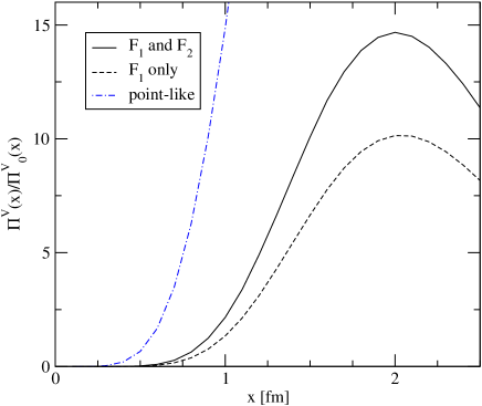
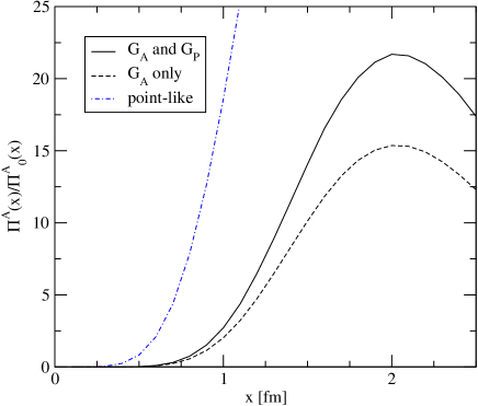
Figure 6.1: Nucleon pole contribution to the vector (upper panel) and axial-vector (lower panel) nucleon three-point function. The solid line shows the complete results, the dashed line is the contribution from the $F_{1}$ and $G_{A}$ form factors only, and the dash-dotted line corresponds to a point-like nucleon. We have used a nucleon coupling constant $\lambda=2.2\,{\rm fm}^{-3}$ as well as phenomenological values for the form factors and coupling constants.

In Fig. 6.1 we show the nucleon pole contribution to the vector and axial-vector three-point functions. We have used the phenomenological values of the iso-vector coupling constants

$$\begin{array}[]{rclcrcl}G_{E}(0)&=&1,&&G_{M}(0)&=&4.7,\\ G_{A}(0)&=&1.25,&&G_{P}(0)&=&\frac{4M^{2}}{m_{\pi}^{2}}g_{A}.\end{array}$$ (6.37)

We have parametrized $G_{E,V}$ and $G_{A}$ by dipole functions with $m_{V}=0.88$ GeV and $m_{A}=1.1$ GeV. The induced pseudoscalar form factor is parametrized as a pion propagator multiplied by a dipole form factor with dipole mass $m_{A}$.

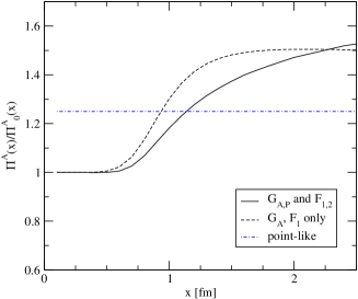
Figure 6.2: Ratio of the phenomenological parameterizations of the axial-vector and vector three-point functions. We have added a short distance continuum contribution to the nucleon pole terms. The curves are labeled as in the previous figure. Note that both the solid and the dashed line will approach $g_{A}=1.25$ as $x\to\infty$. Also note that the solid line is in very good agreement with the instanton calculation shown in Fig. 3.13.

We observe that at distances that are accessible in lattice or instanton simulations, $x\sim(1-2)$ fm, the typical momentum transfer is not small and the correlation function is substantially reduced as compared to the result for a point-like nucleon. We also observe that the $F_{2}$ and $G_{P}$ form factors make substantial contributions. Fig. 6.2 shows that the ratio of the axial-vector and vector correlation functions is nevertheless close to the value for a point-like nucleon, $g_{A}/g_{V}\simeq 1.25$. We observe that the ratio of point-to-point correlation functions approaches this value from above. This is related to the fact that the axial radius of the nucleon is smaller than the vector radius. As a consequence, the point-to-point correlation function at finite separation $\tau$ “sees” a larger fraction of the axial charge as compared to the vector charge.

6.2 Instanton contribution to quark three-point functions

In this appendix we provide the results for the traces that appear in the single instanton contribution to the quark three-point function. Our starting point is the expression

$$(P^{con}_{A/VQQ})^{\mu\nu}=P_{NZNZ}^{\mu\nu}+c_{A/V}\left(P^{\mu\nu}_{ZMm}+P^{\mu\nu}_{mZM}\right),$$ (6.38)

see equ. (3.61). Due to the Dirac structure of the non-zero mode part of the propagator, the $NZNZ$ term is the same for both the vector and axial-vector correlation functions. It has 4 parts stemming from combinations of the two terms of non-zero mode propagator equ. 3.17

$$P_{NZNZ_{11}}^{\mu\nu} = \frac{2H(x,z,y)(x-z)^{\alpha}(z-y)^{\beta}}{\pi^{4}(x-z)^{4}(z-y)^{4}}S^{\nu\alpha\mu\beta}$$ (6.39)

$$\times\left[1+\frac{\rho^{2}}{z^{2}}\left(\frac{x\cdot z}{x^{2}}+\frac{z\cdot y}{y^{2}}\right)+\frac{\rho^{4}x\cdot y}{x^{2}z^{2}y^{2}}\right],$$

$$P_{NZNZ_{12}}^{\mu\nu} = \frac{H(x,z,y)(x-z)^{\alpha}y^{\beta}}{2\pi^{4}(x-z)^{4}(z-y)^{2}z^{2}y^{2}}[(z^{\alpha_{0}}+\frac{\rho^{2}}{x^{2}}x^{\alpha_{0}})S^{\alpha_{0}\sigma\sigma_{0}\beta}\pm\frac{\rho^{2}}{x^{2}}x^{\alpha_{0}}\epsilon^{\alpha_{0}\sigma\sigma_{0}\beta}]$$

$$\times\left[\frac{\rho^{2}(z-y)^{\sigma_{0}}}{\rho^{2}+z^{2}}(S^{\nu\alpha\mu\sigma}\pm\epsilon^{\nu\alpha\mu\sigma})+\frac{\rho^{2}(z-y)^{\sigma}}{\rho^{2}+y^{2}}(S^{\nu\alpha\mu\sigma_{0}}\mp\epsilon^{\nu\alpha\mu\sigma_{0}})\right],$$

$$P_{NZNZ_{21}}^{\mu\nu} = \frac{H(x,z,y)(z-y)^{\alpha}x^{\beta}}{2\pi^{4}(x-z)^{2}(z-y)^{4}z^{2}x^{2}}[(z^{\alpha_{0}}+\frac{\rho^{2}}{y^{2}}y^{\alpha_{0}})S^{\beta\sigma\sigma_{0}\alpha_{0}}\pm\frac{\rho^{2}}{y^{2}}y^{\alpha_{0}}\epsilon^{\beta\sigma\sigma_{0}\alpha_{0}}]$$

$$\times\left[\frac{\rho^{2}(x-z)^{\sigma_{0}}}{\rho^{2}+x^{2}}(S^{\nu\sigma\mu\alpha}\pm\epsilon^{\nu\sigma\mu\alpha})+\frac{\rho^{2}(x-z)^{\sigma}}{\rho^{2}+z^{2}}(S^{\nu\sigma_{0}\mu\alpha}\mp\epsilon^{\nu\sigma_{0}\mu\alpha})\right],$$

$$P_{NZNZ_{22}}^{\mu\nu} = \frac{H(x,z,y)x^{\alpha_{0}}y^{\beta}}{4\pi^{4}(x-z)^{2}(z-y)^{2}z^{2}y^{2}x^{2}}\frac{\rho^{4}}{(\rho^{2}+z^{2})}T_{\pm}[\alpha_{0},\alpha,\sigma,\alpha_{1},\sigma_{1},\beta]$$ (6.42)

$$\times\left[\frac{(x-z)^{\sigma}(z-y)^{\sigma_{1}}}{(\rho^{2}+x^{2})}(S^{\nu\alpha\mu\alpha_{1}}\pm\epsilon^{\nu\alpha\mu\alpha_{1}})\right.$$

$$\hskip 28.45274pt+\left.\frac{(x-z)^{\alpha}(z-y)^{\alpha_{1}}}{(\rho^{2}+y^{2})}(S^{\nu\sigma\mu\sigma_{1}}\mp\epsilon^{\nu\sigma\mu\sigma_{1}})\right],$$

where

$$H(x,z,y)=\left\{\left(1+\frac{\rho^{2}}{z^{2}}\right)\sqrt{\left(1+\frac{\rho^{2}}{x^{2}}\right)\left(1+\frac{\rho^{2}}{y^{2}}\right)}\right\}^{-1}$$ (6.43)

and the Dirac trace $T_{\pm}$ is defined as

$$T_{\mp}[\mu,2,3,4,5,6] \equiv \left(g^{\mu 2}S^{3456}-g^{\mu 3}S^{2456}+g^{\mu 4}S^{2356}-g^{\mu 5}S^{2346}+g^{\mu 6}S^{2345}\right)$$ (6.44)

$$\mp\left(g^{\mu 2}\epsilon^{3456}-g^{\mu 3}\epsilon^{2456}+g^{23}\epsilon^{\mu 456}+g^{45}\epsilon^{\mu 236}-g^{46}\epsilon^{\mu 235}+g^{56}\epsilon^{\mu 234}\right),$$

where $2,3,\ldots$ is short for $\mu_{2},\mu_{3},\ldots$. The $S_{ZM}S_{m}$ term is easily seen to be

$$P^{\mu\nu}_{ZMm} = {\rm Tr}[-\Psi_{0}(x)\Psi_{0}^{+}(z)\gamma^{\mu}(-\Delta_{\pm}(z,y)\gamma_{\pm})\gamma^{\nu}]$$ (6.45)

$$= \frac{\varphi(x)\varphi(z)x^{\alpha_{0}}z^{\beta_{0}}}{8\pi^{2}(z-y)^{2}}\frac{1}{\sqrt{(1+\frac{\rho^{2}}{z^{2}})(1+\frac{\rho^{2}}{y^{2}})}}T_{\mp}[\alpha_{0},\sigma_{1},\sigma,\beta_{0},\mu,\nu]$$

$$\times\left[\delta^{\sigma_{1},\sigma}+\frac{\rho^{2}z^{\alpha}y^{\beta}}{z^{2}y^{2}}(S^{\sigma_{1}\sigma\alpha\beta}\pm\epsilon^{\sigma_{1}\sigma\alpha\beta})\right]$$

with $\varphi(x)=\rho/(\pi\sqrt{x}(x^{2}+\rho^{2})^{3/2})$. The $S_{m}S_{ZM}$ term is obtained similarly

$$P^{\mu\nu}_{mZM} = {\rm Tr}[(-\Delta_{\pm}(x,z)\gamma_{\pm})\gamma^{\mu}(-\Psi_{0}(z)\Psi_{0}^{+}(y))\gamma^{\nu}]$$ (6.46)

$$= \frac{\varphi(z)\varphi(y)z^{\alpha_{0}}y^{\beta_{0}}}{8\pi^{2}(x-z)^{2}}\frac{1}{\sqrt{(1+\frac{\rho^{2}}{x^{2}})(1+\frac{\rho^{2}}{z^{2}})}}T_{\mp}[\alpha_{0},\sigma_{1},\sigma,\beta_{0},\nu,\mu]\times$$

$$\times\left[\delta^{\sigma_{1},\sigma}+\frac{\rho^{2}x^{\alpha}z^{\beta}}{x^{2}z^{2}}(S^{\sigma_{1}\sigma\alpha\beta}\pm\epsilon^{\sigma_{1}\sigma\alpha\beta})\right].$$

For all the above formulas, we need to add instanton and anti-instanton contribution and integrate over the position of the instanton, which was suppressed above. As usual, for an instanton at position $z_{I}$ we have to shift $x,y,z$ according to $x\to(x-z_{I})$, etc.

6.2.1 Computation of path exponent

The correlation functions of operators at different points are made gauge invariant by introducing the connector, the Wilson line. In this appendix we compute the Wilson line in instanton background.

In order to perform the computation, we need to evaluate the path exponent

$$P.e.=Pexp(i\int_{x1}^{x2}A^{\nu,a}\tau^{a}dx^{\nu})$$ (6.47)

For a general gauge configuration that is not an easy task as the path exponent is defined as follows. Parametrize the path by $s\in[0,1]$. The integral in the exponent is then a limit of a sum of matrices, which might not commute. Expand the exponential in power series and reorder the matrices in each term in decreasing value of parameter s. The sum obtained this way is the well-known Wilson line.

For the path exponent along a straight line in the field of an instanton the computation is actually much simpler. Let us parametrize the line by $x^{\mu}=x_{1}^{\mu}+s(x_{2}-x_{1})^{\mu}$, so that the end points $x_{1}$ and $x_{2}$ correspond to $s=0$ and $s=1$ respectively. The integral then reads:

$$\int_{x_{1}}^{x_{2}}A^{a,\mu}_{\pm}\tau^{a}dx^{\mu} = \int_{0}^{1}\eta\!\!\!\!\!-^{a}_{\mu\nu}\tau^{a}\frac{\rho^{2}\,x^{\nu}(s)}{x^{2}(s)(x^{2}(s)+\rho^{2})}\frac{dx^{\mu}}{ds}ds$$

$$= \int_{0}^{1}\eta\!\!\!\!\!-^{a}_{\mu\nu}\tau^{a}\frac{\rho^{2}\left[x_{1}^{\nu}(x_{2}-x_{1})^{\mu}+s(x_{2}-x_{1})^{\nu}(x_{2}-x_{1})^{\mu}\right]}{(x_{1}+s(x_{2}-x_{1}))^{2}(x_{1}+s(x_{2}-x_{1}))^{2}+\rho^{2})}ds,$$

with $\tau^{a}$ Pauli matrices.

The second term in the numerator vanishes due to the anti-symmetry of t’Hooft’s tensor $\eta^{a}_{\mu\nu}=-\eta^{a}_{\nu\mu}$. Then the integrand is in fact a constant matrix multiplied by a function of $s$ at any point on the line. As a result, no path-ordering is necessary since the matrices at any point commute. Therefore we can integrate first and then expand the exponential to get:

$$\int_{x_{1}}^{x_{2}}A^{a,\mu}_{\pm}\tau^{a}dx^{\mu} \equiv \tau^{a}K^{a}_{\pm}=\tau^{a}\eta\!\!\!\!\!-^{a}_{\mu\nu}x_{1}^{\nu}(x_{2}-x_{1})^{\mu}$$ (6.48)

$$\times \left\{\Omega_{1}(x_{1},x_{2})\left[\tan^{-1}\left(x_{2}\cdot(x_{2}-x_{1})\Omega_{1}(x_{1},x_{2})\right)\right.\right.$$

$$\hskip 34.14322pt\left.-\tan^{-1}\left(x_{1}\cdot(x_{2}-x_{1})\Omega_{1}(x_{1},x_{2})\right)\right]$$

$$- \Omega_{2}(x_{1},x_{2},\rho)\left[\tan^{-1}\left(x_{2}\cdot(x_{2}-x_{1})\Omega_{2}(x_{1},x_{2},\rho)\right)\right.$$

$$\hskip 34.14322pt\left.\left.-\tan^{-1}\left(x_{1}\cdot(x_{2}-x_{1})\Omega_{2}(x_{1},x_{2},\rho)\right)\right]\right\}$$

where

$$\Omega_{1}(x_{1},x_{2}) = \frac{1}{\sqrt{x_{1}^{2}(x_{2}-x_{1})^{2}-(x_{1}\cdot(x_{2}-x_{1}))^{2}}}$$

$$\Omega_{2}(x_{1},x_{2},\rho) = \frac{1}{\sqrt{(\rho^{2}+x_{1}^{2})(x_{2}-x_{1})^{2}-(x_{1}\cdot(x_{2}-x_{1}))^{2}}}$$

The expansion of the exponent of Pauli matrices is then easy:

$$Pexp\left(i\int_{x_{1}}^{x_{2}}A^{a,\mu}_{\pm}\tau^{a}dx^{\mu}\right) = \cos\left[\left|K_{\pm}(x_{1},x_{2})\right|\right]$$ (6.49)

$$+i\sin\left[\left|K_{\pm}(x_{1},x_{2})\right|\right]\Omega_{1}(x_{1},x_{2})\eta\!\!\!\!\!-^{a}_{\mu\nu}x_{1}^{\nu}(x_{2}-x_{1})^{\mu}\tau^{a}$$

where the modulus of $K^{a}(x_{1},x_{2})$ is

$$\left|K(x_{1},x_{2})\right| = \sqrt{K^{a}K^{a}}$$ (6.50)

$$= \left\{\tan^{-1}\left(x_{2}\cdot(x_{2}-x_{1})\Omega_{1}(x_{1},x_{2})\right)\right.$$

$$\hskip 42.67912pt-\tan^{-1}\left(x_{1}\cdot(x_{2}-x_{1})\Omega_{1}(x_{1},x_{2})\right)$$

$$-\frac{\Omega_{2}(x_{1},x_{2},\rho)}{\Omega_{1}(x_{1},x_{2})}\left(\tan^{-1}\left(x_{2}\cdot(x_{2}-x_{1})\Omega_{2}(x_{1},x_{2},\rho)\right)\right.$$

$$\hskip 42.67912pt-\left.\left.\tan^{-1}\left(x_{1}\cdot(x_{2}-x_{1})\Omega_{2}(x_{1},x_{2},\rho)\right)\right)\right\}$$

In the above formulas we took the instanton to be centered at 0. The generalization to instanton center at z is straight-forwardly obtained by the replacement $x_{1}\to x_{1}-z$ and $x_{2}\to x_{2}-z$.

For example, for the case of an infinite line in 4-direction we get:

$$Pexp\left(i\int_{-\infty}^{+\infty}A^{a,4}_{\pm}\tau^{a}dx^{4}\right) = \cos{\left[\pi(1-\frac{|\vec{z}|}{\sqrt{|\vec{z}|^{2}+\rho^{2}}})\right]}$$ (6.51)

$$- i\sin{\left[\pi(1-\frac{|\vec{z}|}{\sqrt{|\vec{z}|^{2}+\rho^{2}}})\right]}\frac{\vec{z}}{|\vec{z}|}\cdot\vec{\tau}$$

in agreement with formula (206) of [24].

6.3 Euclidean matrices, conventions, ..

We use the following conventions:

$$g^{\mu\nu} = \delta^{\mu\nu}=diag(1,1,1,1)=g_{\mu\nu},$$

$$\epsilon^{1234} = \epsilon_{1234}=+1$$

The contractions of $\epsilon$ therefore are

$$\epsilon_{\rho\nu\alpha\beta}\epsilon^{\rho\mu\sigma\sigma^{\prime}}=\left|\begin{tabular}[]{c c c}$\delta^{\mu}_{\nu}$&$\delta^{\mu}_{\alpha}$&$\delta^{\mu}_{\beta}$\\ $\delta^{\sigma}_{\nu}$&$\delta^{\sigma}_{\alpha}$&$\delta^{\sigma}_{\beta}$\\ $\delta^{\sigma^{\prime}}_{\nu}$&$\delta^{\sigma^{\prime}}_{\alpha}$&$\delta^{\sigma^{\prime}}_{\beta}$\end{tabular}\right|$$ (6.52)

and $\epsilon_{\rho\rho^{\prime}\alpha\beta}\epsilon^{\rho\rho^{\prime}\mu\nu}=2(\delta^{\mu}_{\alpha}\delta^{\nu}_{\beta}-\delta^{\nu}_{\alpha}\delta^{\mu}_{\beta})$, $\epsilon_{\rho\rho^{\prime}\alpha\beta}\epsilon^{\rho\rho^{\prime}\alpha\nu}=6\delta^{\nu}_{\beta}$ and $\epsilon_{\rho\rho^{\prime}\alpha\beta}\epsilon^{\rho\rho^{\prime}\alpha\beta}=24$

Euclidean gamma matrices are defined as $\{\gamma^{\mu},\gamma^{\nu}\}=2g^{\mu\nu}$. We take $\gamma^{5}=\gamma^{1}\gamma^{2}\gamma^{3}\gamma^{4}$ and $\sigma^{\mu\nu}=\frac{1}{2}[\gamma^{\mu},\gamma^{\nu}]$. The following relations apply: $\gamma_{\mu}^{\dagger}=\gamma_{\mu}$, $\gamma_{5}\sigma^{\mu\nu}=-\frac{1}{2}\epsilon^{\mu\nu\alpha\beta}\sigma_{\alpha\beta}$ One can easily compute the traces:

$$Tr[\gamma^{\mu}\gamma^{\nu}] = 4g^{\mu\nu}$$

$$Tr[\gamma^{\mu}\gamma^{\sigma}\gamma^{\nu}\gamma^{\rho}] = 4(g^{\mu\sigma}g^{\nu\rho}-g^{\mu\nu}g^{\rho\sigma}+g^{\mu\rho}g^{\sigma\nu})\equiv 4S^{\mu\sigma\nu\rho}$$

$$Tr[\gamma^{\mu}\gamma^{\sigma}\gamma^{\nu}\gamma^{\rho}\gamma^{5}] = 4\epsilon^{\mu\sigma\nu\rho}$$

$$Tr[\gamma^{\mu}\gamma^{\sigma}\gamma^{\rho}\gamma^{\rho^{\prime}}\gamma^{\sigma^{\prime}}\gamma^{\nu}] = 4\left[g^{\mu\sigma}S^{\rho\rho^{\prime}\sigma^{\prime}\nu}-g^{\mu\rho}S^{\sigma\rho^{\prime}\sigma^{\prime}\nu}+g^{\mu\rho^{\prime}}S^{\sigma\rho\sigma^{\prime}\nu}\right.$$

$$\hskip 42.67912pt\left.-g^{\mu\sigma^{\prime}}S^{\sigma\rho\rho^{\prime}\nu}+g^{\mu\nu}S^{\sigma\rho\rho^{\prime}\sigma^{\prime}}\right]$$

$$Tr[\gamma^{\mu}\gamma^{\sigma}\gamma^{\rho}\gamma^{\rho^{\prime}}\gamma^{\sigma^{\prime}}\gamma^{\nu}\gamma^{5}] = 4\left[\epsilon^{\mu\sigma\rho\nu^{\prime}}S^{\nu^{\prime}\rho^{\prime}\sigma^{\prime}\nu}+S^{\mu\sigma\rho\nu^{\prime}}\epsilon^{\nu^{\prime}\rho^{\prime}\sigma^{\prime}\nu}\right]$$ (6.53)

Some useful decomposition:(for transparency we will short our notation from $\gamma^{\mu_{1}}\to\gamma^{1}$)

$$\gamma^{1}\gamma^{2}\gamma^{3}\gamma^{4}\gamma^{5}\gamma^{6}\gamma_{\mp}=\gamma_{\mp}(g^{1\mu}+\sigma^{1\mu})T_{\mp}[\mu,2,3,4,5,6]$$ (6.54)

where the Dirac trace $T_{\mp}$ was defined in 6.44. The four vector of $SU(2)_{c}$ matrices is $\sigma^{\mu}_{\pm}=(\vec{\sigma},\mp i)$ while the color - rotated matrices are given as $\sigma^{\mu}_{\pm}(R)=(R^{ab}{\sigma}^{b},\mp i)$. Here $R^{ab}$ is the adjoint representation rotation matrix, defined as $R^{ab}\sigma^{b}=U\sigma^{a}U^{\dagger}$, with $U\in SU(2)$. The following relations link the $SU(2)$ generators to t’Hooft $\eta$ tensor:

$$\sigma^{\mu}_{+}\sigma^{\nu}_{-} = g^{\mu\nu}+i\eta^{a,\mu\nu}R^{ab}\sigma^{b}$$

$$\sigma^{\mu}_{-}\sigma^{\nu}_{+} = g^{\mu\nu}+i\bar{\eta}^{a,\mu\nu}R^{ab}\sigma^{b}$$ (6.55)

The definition and useful properties of $\eta$ can be found e.g. in [24]. For our computations suffices to list the most often used formulas:

$$\eta\!\!\!\!\!-^{a}_{\mu\nu}\eta\!\!\!\!\!-^{a}_{\rho\lambda} = \delta_{\mu\rho}\delta_{\nu\lambda}-\delta_{\mu\lambda}\delta_{\nu\rho}\mp\epsilon_{\mu\nu\rho\lambda}$$ (6.56)

$$\epsilon^{abc}\eta\!\!\!\!\!-^{a}_{\alpha\beta}\eta\!\!\!\!\!-^{b}_{\mu\nu}\eta\!\!\!\!\!-^{c}_{\rho\lambda} = \delta_{\mu\rho}\eta\!\!\!\!\!-^{a}_{\alpha\beta}\eta\!\!\!\!\!-^{a}_{\nu\lambda}-\delta_{\mu\lambda}\eta\!\!\!\!\!-^{a}_{\alpha\beta}\eta\!\!\!\!\!-^{a}_{\nu\rho}+\delta_{\nu\lambda}\eta\!\!\!\!\!-^{a}_{\mu\rho}\eta\!\!\!\!\!-^{a}_{\alpha\beta}-\delta_{\nu\rho}\eta\!\!\!\!\!-^{a}_{\mu\lambda}\eta\!\!\!\!\!-^{a}_{\alpha\beta}$$

where $\eta\!\!\!\!\!-$ is $\bar{\eta}$ ($\eta$) for upper (lower) sign.

After tracing the color indices, all the rotation matrices cancel due to orthogonality $R^{ab}R^{cb}=\delta^{ac}$ and unimodularity $\det R=1$. The following traces are therefore also valid for color-rotated matrices.

$$Tr[\sigma^{\mu}_{+}\sigma^{\nu}_{-}]=Tr[\sigma^{\mu}_{-}\sigma^{\nu}_{+}]=2\delta^{\mu\nu}$$ (6.57)

$$Tr[\sigma^{\mu}_{\pm}\sigma^{\nu}_{\mp}\sigma^{\rho}_{\pm}\sigma^{\sigma}_{\mp}]=2(S^{\mu\nu\rho\sigma}\mp\epsilon^{\mu\nu\rho\sigma})$$ (6.58)

As one can easily see, the traces of $SU(2)$ matrices $Tr[\sigma^{\mu}_{\pm}\cdots]$ can be obtained from the traces of corresponding $\gamma$ matrices projected to the particular 2x2 submatrix as follows: $Tr_{c}[\sigma^{\mu}_{\pm}\cdots\sigma^{\nu}_{\mp}]=Tr_{D}[(\gamma^{\mu}\cdots\gamma^{\nu})\gamma_{\mp}]$

We also provide some useful decompositions for the multiplication of color matrices:

$$\sigma^{\rho}_{\mp}\sigma^{\sigma}_{\pm}\sigma^{\mu}_{\mp}\sigma^{\nu}_{\pm}=\delta^{\rho\sigma}\delta^{\mu\nu}-\eta\!\!\!\!\!-^{a,\rho\sigma}\eta\!\!\!\!\!-^{a,\mu\nu}+i\sigma^{a}\Bigl{[}\eta\!\!\!\!\!-^{a,\rho\sigma}\delta^{\mu\nu}+\eta\!\!\!\!\!-^{a,\mu\nu}\delta^{\rho\sigma}-\eta\!\!\!\!\!-^{b,\rho\sigma}\eta\!\!\!\!\!-^{c,\mu\nu}\epsilon^{bca}\Bigr{]}$$ (6.59)

$$\sigma^{\mu}_{\mp}\sigma^{\nu}_{\pm}\sigma^{\alpha}_{\mp}\sigma^{\beta}_{\pm}\sigma^{\rho}_{\mp}\sigma^{\sigma}_{\pm} = {\bf{1}}\Bigl{\{}\delta^{\mu\nu}\delta^{\alpha\beta}\delta^{\rho\sigma}-\delta^{\mu\nu}\eta\!\!\!\!\!-^{a,\alpha\beta}\eta\!\!\!\!\!-^{a,\rho\sigma}\Bigr{.}$$

$$\hskip 14.22636pt-\;\Bigl{.}\eta\!\!\!\!\!-^{c,\mu\nu}\Bigl{[}\eta\!\!\!\!\!-^{c,\alpha\beta}\delta^{\rho\sigma}+\eta\!\!\!\!\!-^{c,\rho\sigma}\delta^{\alpha\beta}-\eta\!\!\!\!\!-^{a,\alpha\beta}\eta\!\!\!\!\!-^{b,\rho\sigma}\epsilon^{abc}\Bigr{]}\Bigr{\}}$$

$$+i\sigma^{b}\Bigl{\{}\eta\!\!\!\!\!-^{b,\mu\nu}(\delta^{\alpha\beta}\delta^{\rho\sigma}-\eta\!\!\!\!\!-^{a,\alpha\beta}\eta\!\!\!\!\!-^{a,\rho\sigma})\Bigr{.}$$

$$\hskip 14.22636pt-\;\Bigl{.}\epsilon^{ecb}\eta\!\!\!\!\!-^{e,\mu\nu}[\eta\!\!\!\!\!-^{c,\alpha\beta}\delta^{\rho\sigma}+\eta\!\!\!\!\!-^{c,\rho\sigma}\delta^{\alpha\beta}-\eta\!\!\!\!\!-^{a,\alpha\beta}\eta\!\!\!\!\!-^{a^{\prime},\rho\sigma}\epsilon^{aa^{\prime}c}]\Bigr{\}}$$

References

• [1] A. A. Belavin, A. M. Polyakov, A. S. Shvarts and Y. S. Tyupkin, Phys. Lett. B 59, 85 (1975).
• [2] G. ’t Hooft, Phys. Rev. D 14, 3432 (1976) [Erratum-ibid. D 18, 2199 (1978)].
• [3] A. V. Yung, Nucl. Phys. B 297, 47 (1988).
• [4] I. I. Balitsky and A. V. Yung, Phys. Lett. B 168, 113 (1986).
• [5] H. Aoyama, T. Harano, M. Sato and S. Wada, Nucl. Phys. B 466, 127 (1996) [arXiv:hep-th/9512064].
• [6] I. Affleck, Nucl. Phys. B 191, 429 (1981).
• [7] N.K.Nielsen, M.Nielsen, Phys. Rev. D 61, 105020 2000
• [8] P. Faccioli and E. V. Shuryak, Phys. Rev. D 64, 114020 (2001) [arXiv:hep-ph/0106019].
• [9] V. A. Novikov, L. B. Okun, M. A. Shifman, A. I. Vainshtein, M. B. Voloshin and V. I. Zakharov, Phys. Rept.  41, 1 (1978).
• [10] M. A. Shifman, Z. Phys. C 4, 345 (1980) [Erratum-ibid. C 6, 282 (1980)].
• [11] T. Appelquist and H. D. Politzer, Phys. Rev. Lett.  34, 43 (1975); A. De Rujula and S. L. Glashow, Phys. Rev. Lett.  34, 46 (1975).
• [12] G. T. Bodwin, E. Braaten and G. P. Lepage, Phys. Rev. D 51, 1125 (1995) [Erratum-ibid. D 55, 5853 (1997)] [hep-ph/9407339].
• [13] K. Gottfried, Phys. Rev. Lett.  40, 598 (1978).
• [14] M. B. Voloshin, Nucl. Phys. B 154, 365 (1979).
• [15] S. J. Brodsky and G. P. Lepage, Phys. Rev. D 24, 2848 (1981).
• [16] V. L. Chernyak and A. R. Zhitnitsky, Phys. Rept.  112, 173 (1984).
• [17] M. Anselmino, M. Genovese and D. E. Kharzeev, Phys. Rev. D 50, 595 (1994) [hep-ph/9310344].
• [18] J. D. Bjorken, preprint, hep-ph/0008048.
• [19] I. I. Balitsky and V. M. Braun, Phys. Lett. B 314 (1993) 237 [hep-ph/9305269].
• [20] S. Moch, A. Ringwald and F. Schrempp, Nucl. Phys. B 507 (1997) 134 [hep-ph/9609445].
• [21] N. I. Kochelev and V. Vento, Phys. Rev. Lett.  87, 111601 (2001) [hep-ph/0101337].
• [22] N. I. Kochelev, V. Vento and A. V. Vinnikov, Phys. Lett. B 472, 247 (2000) [hep-ph/9905438].
• [23] D. Diakonov, Proceedings of the International School of Physics, ’Enrico Fermi’, Course 80: Selected Topics in Nonperturbative QCD, Varenna, Italy, 1995, [hep-ph/9602375].
• [24] T. Schäfer and E. V. Shuryak, Rev. Mod. Phys.  70, 323 (1998) [hep-ph/9610451].
• [25] C. G. Callan, R. F. Dashen, D. J. Gross, F. Wilczek and A. Zee, Phys. Rev. D 18, 4684 (1978).
• [26] C. G. Callan, R. F. Dashen and D. J. Gross, Phys. Rev. D 17, 2717 (1978).
• [27] G. ’t Hooft, Phys. Rev. Lett. 37, 8 (1976).
• [28] M. A. Shifman, A. I. Vainshtein and V. I. Zakharov, Nucl. Phys. B 165, 45 (1980).
• [29] M. A. Shifman, A. I. Vainshtein and V. I. Zakharov, Nucl. Phys. B 163, 46 (1980).
• [30] K. Hagiwara et al. [Particle Data Group Collaboration], Phys. Rev. D 66, 010001 (2002).
• [31] S. Narison, preprint, hep-ph/0202200.
• [32] T. Feldmann, Int. J. Mod. Phys. A 15, 159 (2000) [hep-ph/9907491].
• [33] V. A. Novikov, M. A. Shifman, A. I. Vainshtein and V. I. Zakharov, Nucl. Phys. B 165, 67 (1980).
• [34] S. Narison, Nucl. Phys. B 509, 312 (1998) [hep-ph/9612457].
• [35] T. Schäfer and E. V. Shuryak, Phys. Rev. Lett.  75, 1707 (1995) [hep-ph/9410372].
• [36] C. Michael and P. S. Spencer, Phys. Rev. D 52, 4691 (1995) [hep-lat/9503018].
• [37] D. A. Smith and M. J. Teper [UKQCD collaboration], Phys. Rev. D 58, 014505 (1998) [hep-lat/9801008].
• [38] P. de Forcrand, M. Garcia Perez and I. O. Stamatescu, Nucl. Phys. B 499, 409 (1997) [hep-lat/9701012].
• [39] T. DeGrand, A. Hasenfratz and T. G. Kovacs, Nucl. Phys. B 505, 417 (1997) [hep-lat/9705009].
• [40] J. Sexton, A. Vaccarino and D. Weingarten, Phys. Rev. Lett.  75, 4563 (1995) [hep-lat/9510022].
• [41] W. J. Lee and D. Weingarten, Phys. Rev. D 61, 014015 (2000) [hep-lat/9910008].
• [42] P. Minkowski and W. Ochs, Eur. Phys. J. C 9, 283 (1999) [hep-ph/9811518].
• [43] F. E. Close, G. R. Farrar and Z. p. Li, Phys. Rev. D 55, 5749 (1997) [hep-ph/9610280].
• [44] M. Franz, M. V. Polyakov and K. Goeke, Phys. Rev. D 62, 074024 (2000) [hep-ph/0002240].
• [45] V. A. Novikov, M. A. Shifman, A. I. Vainshtein and V. I. Zakharov, Nucl. Phys. B 165, 55 (1980).
• [46] R. Partridge et al., Phys. Rev. Lett.  45, 1150 (1980).
• [47] R. M. Baltrusaitis et al. [Mark-III Collaboration], Phys. Rev. D 33, 629 (1986).
• [48] E. V. Shuryak and J. J. M. Verbaarschot, Nucl. Phys. B 410, 55 (1993) [hep-ph/9302239].
• [49] M. Anselmino and S. Forte, Phys. Lett. B 323, 71 (1994) [hep-ph/9311365].
• [50] M. A. Shifman, Phys. Rept.  209, 341 (1991).
• [51] M. Jaminon, M. Mathot and B. van den Bossche, Nucl. Phys. A 662, 157 (2000)
• [52] H. y. Jin, X. m. Zhang, Phys. Rev. D 66, 057505 (2002) [hep-ph/0208120].
• [53] A. Ringwald, Nucl. Phys. B 330 (1990) 1.
• [54] O. Espinosa, Nucl. Phys. B 343 (1990) 310.
• [55] M. A. Nowak, E. V. Shuryak and I. Zahed, Phys. Rev. D 64, 034008 (2001) [hep-ph/0012232].
• [56] J. Ashman et al. [European Muon Collaboration], Phys. Lett. B 206, 364 (1988).
• [57] B. W. Filippone and X. D. Ji, Adv. Nucl. Phys.  26, 1 (2001) [hep-ph/0101224].
• [58] A. E. Dorokhov, N. I. Kochelev and Y. A. Zubov, Int. J. Mod. Phys. A 8, 603 (1993).
• [59] S. D. Bass and A. W. Thomas, Prog. Part. Nucl. Phys.  33, 449 (1994) [hep-ph/9310306].
• [60] S. D. Bass, Acta Phys. Polon. B 34, 5893 (2003) [hep-ph/0311174].
• [61] G. Altarelli and G. G. Ross, Phys. Lett. B 212, 391 (1988).
• [62] R. L. Jaffe and A. Manohar, Nucl. Phys. B 337, 509 (1990).
• [63] M. A. Shifman, A. I. Vainshtein and V. I. Zakharov, Phys. Lett. B 78, 443 (1978).
• [64] A. Anselm, Phys. Lett. B 291, 455 (1992).
• [65] J. H. Kuhn and V. I. Zakharov, Phys. Lett. B 252, 615 (1990).
• [66] S. Narison, G. M. Shore and G. Veneziano, Nucl. Phys. B 433, 209 (1995) [hep-ph/9404277].
• [67] E. V. Shuryak and J. J. Verbaarschot, Phys. Rev. D 52, 295 (1995) [hep-lat/9409020].
• [68] T. Schäfer and E. V. Shuryak, preprint, hep-lat/0005025.
• [69] T. Schäfer, E. V. Shuryak and J. J. Verbaarschot, Nucl. Phys. B 412, 143 (1994) [hep-ph/9306220].
• [70] D. Diakonov, Prog. Part. Nucl. Phys.  51, 173 (2003) [hep-ph/0212026].
• [71] L. S. Brown, R. D. Carlitz, D. B. Creamer and C. K. Lee, Phys. Rev. D 17, 1583 (1978).
• [72] N. Andrei and D. J. Gross, Phys. Rev. D 18, 468 (1978).
• [73] P. Nason and M. Porrati, Nucl. Phys. B 421, 518 (1994) [hep-ph/9302211].
• [74] B. V. Geshkenbein and B. L. Ioffe, Nucl. Phys. B 166, 340 (1980).
• [75] A. E. Dorokhov and W. Broniowski, Eur. Phys. J. C 32, 79 (2003) [hep-ph/0305037].
• [76] M. S. Dubovikov and A. V. Smilga, Nucl. Phys. B 185, 109 (1981).
• [77] T. Schäfer, E. V. Shuryak and J. J. M. Verbaarschot, Phys. Rev. D 51, 1267 (1995) [hep-ph/9406210].
• [78] T. Schäfer and E. V. Shuryak, Phys. Rev. D 53, 6522 (1996) [hep-ph/9509337].
• [79] T. Schäfer and E. V. Shuryak, Phys. Rev. D 54, 1099 (1996) [hep-ph/9512384].
• [80] N. Isgur and H. B. Thacker, Phys. Rev. D 64, 094507 (2001) [hep-lat/0005006].
• [81] S. Weinberg, Phys. Rev. Lett.  67, 3473 (1991).
• [82] U. Vogl and W. Weise, Prog. Part. Nucl. Phys.  27, 195 (1991).
• [83] K. Steininger and W. Weise, Phys. Rev. D 48, 1433 (1993).
• [84] A. E. Dorokhov, preprint, hep-ph/0112332.
• [85] N. I. Kochelev, Phys. Rev. D 57, 5539 (1998) [hep-ph/9711226].
• [86] B. L. Ioffe, Nucl. Phys. B 188, 317 (1981) [Erratum-ibid. B 191, 591 (1981)].
• [87] R. Rapp, T. Schäfer, E. V. Shuryak and M. Velkovsky, Phys. Rev. Lett.  81, 53 (1998) [hep-ph/9711396].
• [88] D. B. Leinweber, Phys. Rev. D 51, 6383 (1995) [nucl-th/9406001].
• [89] M. Anselmino, E. Predazzi, S. Ekelin, S. Fredriksson and D. B. Lichtenberg, Rev. Mod. Phys.  65, 1199 (1993).
• [90] D. Dolgov, R. Brower, J. W. Negele and A. Pochinsky, Nucl. Phys. Proc. Suppl.  73, 300 (1999) [hep-lat/9809132].
• [91] S. J. Dong, J. F. Lagae and K. F. Liu, Phys. Rev. Lett.  75, 2096 (1995) [hep-ph/9502334].
• [92] S. Forte and E. V. Shuryak, Nucl. Phys. B 357, 153 (1991).
• [93] M. Hutter, preprint, hep-ph/9509402.
• [94] M. Kacir, M. Prakash and I. Zahed, Acta Phys. Polon. B 30, 287 (1999) [hep-ph/9602314].
• [95] D. Diakonov, M. V. Polyakov and C. Weiss, Nucl. Phys. B 461, 539 (1996) [hep-ph/9510232].
• [96] D. Diakonov, V. Y. Petrov and P. V. Pobylitsa, Nucl. Phys. B 306, 809 (1988).
• [97] S. J. Brodsky, J. R. Ellis and M. Karliner, Phys. Lett. B 206, 309 (1988).
• [98] A. Blotz, M. V. Polyakov and K. Goeke, Phys. Lett. B 302, 151 (1993).
• [99] P. Faccioli, preprint, hep-ph/0312019.
• [100] L. Maiani and M. Testa, Phys. Lett. B 245, 585 (1990).
• [101] Michael Creutz: Quarks, Gluons and Lattices, Cambridge University Press, Cambridge, 1983
• [102] M.A.Shifman, A.I.Vainshtein, V.I.Zakharov, Nucl.Phys. B 163: 46-56 (1980)
• [103] S.Chernyshev, M.A.Nowak, I. Zahed, Phys.Rev. D 53: 5176 - 5184 (1996)
• [104] T.Prosen, T.H.Seligman, H.A.Weidenmüller, Europhys.Lett. 55(1): 12-18 (2001)
• [105] K.E.Eriksson, N.Svartholm, R.S.Skagerstam, J.Math.Phys. 22: 2276 (1981)
• [106] V.A.Fateev, E.Onofri, Lett.Math.Phys 5: 367 (1981)
• [107] R.Brower, M.Nauenberg, Nucl.Phys. B 180: 221 (1981)
• [108] M. Creutz, J.Math.Phys. 19(10): 2043-2046 (1978), Rev.Mod.Phys. 50(3): 561-571 (1978)
• [109] Jaap Hoek, Phys.Lett. B 102: 129 (1981)
• [110] I.Bars, Physica Scripta 23: 983-986 (1981) and J.Mth.Phys. 21(11): 2676-2681 (1980)
• [111] A.B.Balantekin, Phys.Rev. D 62: 085017 (2000) and A.B.Balantekin, P.Cassak, J.Math.Phys. 43:604-620 (2002)
• [112] V.I.Borodulin, R.N.Rogalyov, S.R.Slabospitsky, hep-ph/9507456
• [113] A.J.Macfarlane, A.Sudbery, P.H.Weisz, Commun. math. Phys. 11: 77-90(1968)
• [114] P.Dittner, Commun. math. Phys. 22: 238-252 (1971)