$B^{0}_{d,s}-\bar{B}^{0}_{d,s}$ mixing in the model III 2HDM

Abstract

In the model III 2HDM there are new CP violating phases which would affect the $B_{d,s}^{0}-\bar{B}_{d,s}^{0}$ mixing. In this paper, we calculate the new physics contributions to the neutral B meson mass splitting $\Delta M_{B_{q}}$ (q=d, s) at the next-to-leading order (NLO) level. Using the high accuracy data and other relevant data, we draw the constraints on the parameter space of the model III 2HDM. Moreover, we calculate the new physics corrections to the ratio $q/p$. It is found that the phase of $(q/p)_{n}$ for $B_{d}$ which is due to the new contributions is very small and consequently in agreement with the measurements of the time dependent CP asymmetry $S_{J/\psi K}$ in $B\to J/\psi K_{S}$. On the contrary, the phase of $(q/p)_{n}$ for $B_{s}$ is large enough to give significant effects on CP violation in the neutral $B_{s}$ system.

I introduction

The neutral B-meson system has been of fundamental importance in testing the Standard Model (SM) picture of flavor changing neutral currents (FCNC) and CP violation and in probing virtual effects from potential new physics beyond SM at low energies. The presentence of CP violation in the neutral B meson system has been established. The measured value babar ; belle ; cdf of the time dependent CP asymmetry $S_{J/\psi K}$ in $B\to J/\psi K_{S}$

$$S_{J/\psi K}=\sin(2\beta(J/\psi K_{S}))_{\rm world-ave}=0.734\pm 0.054.$$ (1)

is in agreement with the prediction in the standard model (SM).

In the $B_{\sl q}^{0}$ (q=d, s) system, we expect model independently that cpviolation

$$\Gamma_{12}\ll M_{12}$$ (2)

where $\Gamma_{12}$ and $M_{12}$ are the off-diagonal terms of $2\times 2$ decay width matrix and mass matrix of $B_{\sl q}^{0}-\bar{B}_{\sl q}^{0}$. Thus one has

$$\frac{q}{p} = -\frac{M_{12}^{\ast}}{|M_{12}|},$$ (3)

$$\Delta M_{B_{\sl q}} = 2|M_{12}|,$$ (4)

where $q$ and $p$ are defined as

$$|B_{L,H}\rangle=p|B^{0}\rangle\pm q|\bar{B}^{0}\rangle$$ (5)

with $B_{L,H}$ denoting the light and heavy meson mass eigenstates, and the normalization condition is

$$|p|^{2}+|q|^{2}=1.$$ (6)

In the SM, one has, according to the box diagram calculation,

$$\frac{q}{p}=-\frac{V_{tb}^{\ast}V_{t{\sl q}}}{V_{tb}V_{t{\sl q}}^{\ast}}.$$ (7)

and the deviation of $|q/p|$ from 1 is $\sim 10^{-3}$ ($10^{-5}$) for $B_{d}$ ($B_{s}$) nir which is unobservably small. Eq. (7) for the $B_{d}^{0}$ system has been verified by measurements of the time dependent CP asymmetry $S_{J/\psi K}$ in $B\to J/\psi K_{S}$, as mentioned above. Therefore, it would give a constraint on parameters of new theoretical models.

As it is obvious from Eq. (4), $B^{0}-\bar{B}^{0}$ mixing is responsible for the small mass differences between the mass eigenstates of neutral B mesons. The results of measurements of the mass splitting $\Delta m_{d}$ have been obtained with high accuracy. The current world averages of $\Delta m_{q}$ ($q=d,\,s$) are as follow pdg2003 ; hfag03

$$\Delta M_{B_{d}} = 0.502\pm 0.007\,ps^{-1}$$

$$\Delta M_{B_{s}} > 14.4\,ps^{-1}$$ (8)

which would impose a stringent constraint on new model building.

In the SM, $B^{0}-\bar{B}^{0}$ mixing is dominated by the box diagrams with two internal t-quarks and W gauge bosons. In new physics models, the box diagrams with one or two W gauge bosons replaced by the new charged scalars or vector bosons and/or top quarks replaced by new fermions can also contribute to $B^{0}-\bar{B}^{0}$ mixing. Using the precision data we can put stringent constrains on the parameter space of a new physics model. In the paper we study $B^{0}-\bar{B}^{0}$ mixing in the model III 2HDM.

It is well-known that in the model III 2HDM the couplings involving Higgs bosons and fermions can have complex phases, the new CP violating phases would affect $B^{0}-\bar{B}^{0}$ mixing. $B^{0}-\bar{B}^{0}$ mixing has extensively been studied in the model III 2HDM during the past years. The charged-Higgs boson contributions to $B^{0}-\bar{B}^{0}$ mixing have been calculated at the leading order for a long time asw80 . In the framework of SM, Ref. buras90 is the first one to present the NLO QCD corrections to $B^{0}-\bar{B}^{0}$ mixing while in conventional model I and model II 2HDM Ref. urban98 is. The possible constraints on the model III 2HDM from the measured parameter $x_{d}=\Delta M_{B}/\Gamma_{B}$ were studied, for example, in Refs. grant95 ; atwood97 ; bck at the LO level. At the NLO level, Ref. xiao has calculated the charged Higgs boson contribution to mass splitting $\Delta M_{B_{d}}$ and drawn the constraints on the parameters of model III in terms of the high precision data, considering the uncertainty of the non-perturbative parameter $f_{B_{d}}\sqrt{\hat{B}_{B_{d}}}$. The effects of the new CP violating phases on $\Delta M_{B_{d}}$ have been taken into account bck . However, in Ref. bck as well as Ref. xiao all new parameters except for $\lambda_{tt,bb}$ in the model III 2HDM are set to be zero. Furthermore, the ratio $q/p$ which is important ingredient to study CP violation in the neutral B system has not been analyzed. In this paper, we will calculate the new physics contributions to $\Delta M_{B_{q}}$ taking into account the effects of the complex phases and keeping all relevant parameters of the model, which are only subjective to constraints from experiments, non zero at the NLO level in the model III 2HDM. By comparing the theoretical predictions with the high accuracy data, we draw the constraints on the free parameters of model III. Moreover, by using the constrained parameters we calculate the contributions of new physics to the ratio $q/p$ in the neutral B system.

The organization of this paper is as follows. In the next section, we describe the model III 2HDM briefly. In Section III, we give the effective Hamiltonian responsible for $B^{0}-\bar{B}^{0}$ mixing and calculate the mass splitting $\Delta M_{B_{q}}$ and the ratio $q/p$ at the NLO level in the model III. The section IV is devoted to numerical results. Finally, we conclude in section V.

II The model III two higgs doublet model

As the simplest extension of the SM, the so-called two-Higgs-doublet models 2hdm ; gunion90 may naturally have flavor changing neutral currents (FCNC’s) mediated by the Higgs bosons at the tree-level, unless an ad hoc discrete symmetry is imposed. In this paper, we shall focus on the model III 2HDM sher87 ; hou92 ; atwood97 . In the model III, there is no discrete symmetry and both the Higgs doublets can couple to the up-type and down-type quarks. In general one can have a Yukawa Lagrangian of the form

$${\cal L}_{Y}=\eta^{U}_{ij}\bar{Q}_{i,L}\tilde{H}_{1}U_{j,R}+\eta^{D}_{ij}\bar{Q}_{i,L}H_{1}D_{j,R}+\xi^{U}_{ij}\bar{Q}_{i,L}\tilde{H}_{2}U_{j,R}+\xi^{D}_{ij}\bar{Q}_{i,L}H_{2}D_{j,R}\,+\,h.c.$$ (9)

where $H_{i}$ ($i=1,2$) are the two Higgs doublets, while $\eta^{U,D}_{i,j}$ and $\xi^{U,D}_{i,j}$ ($i,j=1,2,3$ are family index) are the nondiagonal matrices of the Yukawa couplings. We can choose to express $H_{1}$ and $H_{2}$ in a suitable basis such that only the $\eta_{ij}^{U,D}$ couplings generate the fermion masses, i.e.

$$\langle H_{1}\rangle=\left(\begin{array}[]{c}0\\ {v\over\sqrt{2}}\end{array}\right)\,\,,\,\,\,\,\,\,\,\,\langle H_{2}\rangle=0$$ (10)

Then the two Higgs doublets in the basis are of the form

$$H_{1}=\frac{1}{\sqrt{2}}\left[\left(\begin{array}[]{c}0\\ v+\phi^{0}_{1}\end{array}\right)+\left(\begin{array}[]{c}\sqrt{2}\,G^{+}\\ iG^{0}\end{array}\right)\right]\,\,,\,\,\,\,\,\,\,\,H_{2}=\frac{1}{\sqrt{2}}\left(\begin{array}[]{c}\sqrt{2}\,H^{+}\\ \phi^{0}_{2}+iA^{0}\end{array}\right)$$ (11)

where $H^{\pm}$ are the physical charged-Higgs bosons and $A^{0}$ is the physical CP-odd neutral Higgs boson, $G^{0}$ and $G^{\pm}$ are the Goldstone bosons that would be eaten away in the Higgs mechanism to become the longitudinal components of the weak gauge bosons. The advantage of using the basis is that the first doublet $H_{1}$ corresponds to the scalar doublet of the SM while the new Higgs fields arise from the second doublet $H_{2}$. The $\phi^{0}_{1}$ and $\phi^{0}_{2}$ are not the neutral mass eigenstates but linear combinations of the CP-even neutral Higgs boson mass eigenstates, $H^{0}$ and $h^{0}$:

$$H^{0} = \phi^{0}_{1}\cos\alpha+\phi^{0}_{2}\sin\alpha$$ (12)

$$h^{0} = -\phi^{0}_{1}\sin\alpha+\phi^{0}_{2}\cos\alpha$$

where $\alpha$ is the mixing angle, such that for $\alpha\!=\!0$, ($\phi^{0}_{1}$, $\phi^{0}_{2}$) coincide with the mass eigenstates.

Note that $Q_{i,L}$, $U_{j,R}$ and $D_{j,R}$ in Eq.(9) are weak eigenstates, which can be rotated into mass eigenstates. After the transformation the flavor changing (FC) part of the Yukawa Lagarangian becomes hll

$${\cal L}_{Y,FC}=\hat{\xi}^{U}_{ij}\bar{Q}_{i,L}\tilde{H}_{2}U_{j,R}+\hat{\xi}^{D}_{ij}\bar{Q}_{i,L}H_{2}D_{j,R}\,+\,h.c.$$ (13)

where

$$\hat{\xi}^{U,D}=(V_{L}^{U,D})^{-1}\cdot\xi^{U,D}\cdot V_{R}^{U,D}$$ (14)

in which $V_{L,R}^{U,D}$ are the rotation matrices acting on the up- and down-type quarks, with left or right chirality respectively, so that $V_{CKM}=(V_{L}^{U})^{{\dagger}}V_{L}^{D}$ is the usual Cabibbo-Kobayashi-Maskawa (CKM) matrix. Feynman rules of Yukawa couplings follows from Eq. (13) can be found in, e.g., Refs. atwood97 ; bck . The FCNC couplings are given by the matrices $\hat{\xi}^{U,D}$ and the charged FC couplings are given by

$$\hat{\xi}^{U}_{\rm charged}\! = \!\hat{\xi}^{U}\cdot V_{CKM}$$

$$\hat{\xi}^{D}_{\rm charged}\! = \!V_{CKM}\cdot\hat{\xi}^{D}$$ (15)

Because the definition of the $\xi^{U,D}_{ij}$ couplings is arbitrary, we can take the rotated couplings as the original ones and shall write $\xi^{U,D}$ in stead of $\hat{\xi}^{U,D}$ hereafter. The Cheng-Sher ansatz for $\xi^{U,D}$ is sher87

$$\xi^{U,D}_{ij}=\frac{g\,\sqrt{m_{i}m_{j}}}{\sqrt{2}\,M_{W}}\lambda_{ij},$$ (16)

by which the quark-mass hierarchy ensures that the FCNC within the first two generations are naturally suppressed by the small quark masses, while a larger freedom is allowed for the FCNC involving the third generation. In the ansatz the residual degree of arbitrariness of the FC couplings is expressed through the $\lambda_{ij}$ parameters which are of order one and need to be determined by the available experiments, and they may also be complex. In the paper we choose $\xi^{U,D}$ to be diagonal and set the masses of u and d quark to be zero for the sake of simplicity, so that $\lambda_{ii}$ ($i=c,s,t,b$) are the new free parameters and will enter into the Wilson coefficients relevant to the process.

III $B^{0}-\bar{B}^{0}$ mixing in the model III 2HDM

III.1 Effective Hamiltonian

The most general effective Hamiltonian for $\Delta B=2$ processes beyond the SM can be written as

$${\cal H}_{\rm eff}^{\Delta B=2} = \sum_{i=1}^{5}C_{i}Q_{i}+\sum_{i=1}^{3}\tilde{C}_{i}\tilde{Q}_{i}$$ (17)

with

$$Q_{1} = \bar{q}^{\alpha}_{L}\gamma^{\mu}b^{\alpha}_{L}\bar{q}^{\beta}_{L}\gamma_{\mu}b^{\beta}_{L}$$

$$Q_{2} = \bar{q}^{\alpha}_{R}b^{\alpha}_{L}\bar{q}^{\beta}_{R}b^{\beta}_{L}$$

$$Q_{3} = \bar{q}^{\alpha}_{R}b^{\beta}_{L}\bar{q}^{\beta}_{R}b^{\alpha}_{L}$$

$$Q_{4} = \bar{q}^{\alpha}_{R}b^{\alpha}_{L}\bar{q}^{\beta}_{L}b^{\beta}_{R}$$

$$Q_{5} = \bar{q}^{\alpha}_{R}b^{\beta}_{L}\bar{q}^{\beta}_{L}b^{\alpha}_{R}$$ (18)

where $q=s,\,d$, corresponding to the operators of $B_{s}$ and $B_{d}$ system respectively, $P_{L,R}\equiv(1\mp\gamma_{5})/2$, and $\alpha$, $\beta$ are colour indexes. The tilde operators $\tilde{Q}_{i}$ ($i=1,2,3$) are obtained from $Q_{i}$ correspondingly by exchanging $L\leftrightarrow R$.

At one loop level only the charged scalars are relevant for the box diagrams contributing to the $\bar{B}^{0}-B^{0}$ mixing amplitude. Using the Cheng-Sher ansatz for $\xi^{U,D}$ which we assume in the paper, we rewrite the tree level couplings of $H_{l}^{+}\equiv(H^{+},G^{+})$ notation (where $G^{\pm}$ is the would-be Goldstone boson) as follows

$${\cal{L}}_{int}=H^{+}_{l}\bar{u}_{A}V_{AI}(Y_{L}^{AIl}P_{L}+Y_{R}^{AIl}P_{R})d_{I}+h.c.$$ (19)

where

$$Y_{L}^{AIl}=\frac{e}{\sqrt{2}s_{W}}\frac{m_{u_{A}}}{M_{W}}\times\left\{\begin{array}[]{ll}\,\,\lambda_{AA}^{\ast}&\textrm{ for \, l=1}\\ \,\,\,\,\,1&\textrm{ for \, l=2}\end{array}\right.$$

$$Y_{R}^{AIl}=\frac{e}{\sqrt{2}s_{W}}\frac{m_{d_{I}}}{M_{W}}\times\left\{\begin{array}[]{ll}\,\,-\lambda_{II}&\textrm{ for \, l=1}\\ \,\,\,\,\,-1&\textrm{ for \, l=2}\end{array}\right.$$

with $A=t,c,u$ and $I=b,s,d$.

In terms of the coefficients $Y_{L}^{AIl}$ and $Y_{R}^{AIl}$ we can express the contributions of $H_{l}^{+}$ to the Wilson coefficients $C_{i}$ of the relevant operators responsible for $B^{0}-\bar{B}^{0}$ mixing as follows.

Diagrams with one $W^{\pm}$ and one $H^{\pm}$ give:

$$C_{1}(\mu)=\frac{(V_{AI}^{\ast}V_{AJ})^{2}}{16\pi^{2}}{e^{2}\over 2s^{2}_{W}}\sum_{A}m_{u_{A}}^{2}Y_{L}^{\dagger AI1}Y_{L}^{AJ1}D_{0}(m_{u_{A}}^{2},m_{u_{A}}^{2},M_{W}^{2},M_{H^{+}}^{2})\phantom{aa}$$

$$C_{2}(\mu)=\frac{(V_{AI}^{\ast}V_{AJ})^{2}}{16\pi^{2}}{e^{2}\over 2s^{2}_{W}}\sum_{A}\sum_{l=1}^{2}Y_{R}^{\dagger AIl}Y_{R}^{AJl}4D_{00}(m_{u_{A}}^{2},m_{u_{A}}^{2},M_{W}^{2},m_{H_{l}^{+}}^{2})$$ (20)

where $s_{W}\equiv\sin\theta_{W}$ ($\theta_{W}$ is the Weinberg angle), the definition of the four-point integral functions $D_{0}$ and $D_{00}$ can be found in the Appendix.

Diagrams with two $H_{l}^{\pm}$ give:

$$C_{1}(\mu)=-{1\over 2}\frac{(V_{AI}^{\ast}V_{AJ})^{2}}{16\pi^{2}}\sum_{A}\sum_{l,n}Y_{L}^{\dagger AIl}Y_{L}^{AJn}Y_{L}^{\dagger AIn}Y_{L}^{AJl}D_{00}(m_{u_{A}}^{2},m_{u_{A}}^{2},M_{H^{+}_{l}}^{2},M_{H^{+}_{n}}^{2})\phantom{aa}$$

$$\tilde{C}_{1}(\mu)=-{1\over 2}\frac{(V_{AI}^{\ast}V_{AJ})^{2}}{16\pi^{2}}\sum_{A}\sum_{l,n}^{2}Y_{R}^{\dagger AIl}Y_{R}^{AJn}Y_{R}^{\dagger AIn}Y_{R}^{AJl}D_{00}(m_{u_{A}}^{2},m_{u_{A}}^{2},M_{H^{+}_{l}}^{2},M_{H^{+}_{n}}^{2})\phantom{aa}$$

$$C_{2}(\mu)=-{1\over 2}\frac{(V_{AI}^{\ast}V_{AJ})^{2}}{16\pi^{2}}\sum_{A}\sum_{l,n}^{2}m_{u_{A}}^{2}Y_{R}^{\dagger AIl}Y_{L}^{AJn}Y_{R}^{\dagger AIn}Y_{L}^{AJl}D_{0}(m_{u_{A}}^{2},m_{u_{A}}^{2},M_{H^{+}_{l}}^{2},M_{H^{+}_{n}}^{2})\phantom{aa}$$

$$\tilde{C}_{2}(\mu)=-{1\over 2}\frac{(V_{AI}^{\ast}V_{AJ})^{2}}{16\pi^{2}}\sum_{A}\sum_{l,n}^{2}m_{u_{A}}^{2}Y_{L}^{\dagger AIl}Y_{R}^{AJn}Y_{L}^{\dagger AIn}Y_{R}^{AJl}D_{0}(m_{u_{A}}^{2},m_{u_{A}}^{2},M_{H^{+}_{l}}^{2},M_{H^{+}_{n}}^{2})\phantom{aa}$$

$$C_{4}(\mu)=-\frac{(V_{AI}^{\ast}V_{AJ})^{2}}{16\pi^{2}}\sum_{A}\sum_{l,n}^{2}m_{u_{A}}^{2}Y_{L}^{\dagger AIl}Y_{L}^{AJn}Y_{R}^{\dagger AIn}Y_{R}^{AJl}D_{0}(m_{u_{A}}^{2},m_{u_{A}}^{2},M_{H^{+}_{l}}^{2},M_{H^{+}_{n}}^{2})\phantom{aa}$$

$$C_{5}(\mu)=2\frac{(V_{AI}^{\ast}V_{AJ})^{2}}{16\pi^{2}}\sum_{A}\sum_{l,n}^{2}Y_{L}^{\dagger AIl}Y_{L}^{AJn}Y_{R}^{\dagger AIn}Y_{R}^{AJl}D_{00}(m_{u_{A}}^{2},m_{u_{A}}^{2},M_{H^{+}_{l}}^{2},M_{H^{+}_{n}}^{2})$$ (21)

The above results of the Wilson Coefficients are in agreement with the ones in buras01 , the different sign and factor are due to the different definitions of the four-point integral functions. At one loop level there are no contributions to the Wilson coefficients of the operators $Q_{3}$ and $\tilde{Q}_{3}$.

In order to calculate the NLO QCD corrections to the Wilson coefficients $C_{i}$ in the evolution from the scale of new physics $\mu_{t}$ down to the low hadronic scale $\mu$ ($\sim m_{b}$), one has to solve the corresponding renormalization group equations. The details can be found in Ref. renormalization , with the result

$$C_{r}(m_{b}^{pole})=\sum_{i}\sum_{s}\left(b^{(r,s)}_{i}+\eta\,c^{(r,s)}_{i}\right)\eta^{a_{i}}\,C_{s}(\mu)$$ (22)

where we have set the new physics scale $\mu_{t}=m_{t}$ and $\eta=\alpha_{s}(\mu)/\alpha_{s}(m_{t})$. The magic numbers $a_{i}$, $b_{i}^{(r,s)}$ and $c_{i}^{(r,s)}$ are given in Ref. renormalization .

III.2 The Master Formulae

In terms of the matrix elements of the effective $\Delta B=2$ Hamiltonian we have the neutral B meson mass difference

$$\Delta M_{B_{q}}=2|M_{12}^{(q)}|$$ (23)

and the ratio of mixing parameters

$$(q/p)_{B_{q}}=-exp\left\{-iArg[M_{12}^{(q)}]\right\}$$ (24)

with

$$M_{12}^{(q)}=\langle\bar{B}^{0}_{q}|{\cal{H}}_{eff}(\Delta B=2)|B^{0}_{q}\rangle.$$ (25)

In the SM, the mass splitting $\Delta M_{B_{q}}$ at the NLO level is available buras96

$$\Delta M_{B_{q}}=\frac{G_{F}^{2}M_{W}^{2}}{6\pi^{2}}m_{B_{q}}(\hat{B}_{B_{q}}f_{B_{q}}^{2})\eta_{B}S_{0}(x_{t})|V_{tq}V_{tb}^{\ast}|^{2}$$ (26)

where $S_{0}(x)$ is the Inami-Lim function Inami-Lim , the details of $\hat{B}_{B_{q}}$ and $\eta_{B}$ can be found in Ref. buras96 .

In the framework of model III 2HDM, we need to know the matrix elements of the relevant operators $Q_{i}$ and $\tilde{Q}_{i}$ between neutral B mesons. One defines renormalization

$$\langle\bar{B}_{q}|Q_{1}(\mu)|B_{q}\rangle = \frac{1}{3}m_{B_{q}}f_{B_{q}}^{2}B_{1}^{(q)}(\mu)$$

$$\langle\bar{B}_{q}|Q_{2}(\mu)|B_{q}\rangle = -\frac{5}{24}\left(\frac{m_{B_{q}}}{m_{b}(\mu)+m_{q}(\mu)}\right)^{2}m_{B_{q}}f_{B_{q}}^{2}B_{2}^{(q)}(\mu)$$

$$\langle\bar{B}_{q}|Q_{3}(\mu)|B_{q}\rangle = \frac{1}{24}\left(\frac{m_{B_{q}}}{m_{b}(\mu)+m_{q}(\mu)}\right)^{2}m_{B_{q}}f_{B_{q}}^{2}B_{3}^{(q)}(\mu)$$

$$\langle\bar{B}_{q}|Q_{4}(\mu)|B_{q}\rangle = \frac{1}{4}\left(\frac{m_{B_{q}}}{m_{b}(\mu)+m_{q}(\mu)}\right)^{2}m_{B_{q}}f_{B_{q}}^{2}B_{4}^{(q)}(\mu)$$

$$\langle\bar{B}_{q}|Q_{5}(\mu)|B_{q}\rangle = \frac{1}{12}\left(\frac{m_{B_{q}}}{m_{b}(\mu)+m_{q}(\mu)}\right)^{2}m_{B_{q}}f_{B_{q}}^{2}B_{5}^{(q)}(\mu)$$ (27)

where $f_{B_{q}}$ is the decay constant and $B_{i}$ is the so-called bag factor. The matrix elements of $\tilde{Q}_{1-3}$ are the same as that of $Q_{1-3}$. The lattice calculations of $B_{i}^{(q)}(\mu)$ have been done in Ref.bagpara and the results are

$$B_{1}^{(d)}(m_{b})=0.87(4)^{+5}_{-4}$$

(28)

IV Numerical Analysis

In numerical calculations, the following values of parameters are assumed:

$$m_{B_{d}}=5.279\,GeV,\;\;m_{B_{s}}=5.370\,GeV,\;\;m_{H^{\pm}}=200\,GeV$$ (29)

The values of $f_{B_{q}}$ and $\hat{B}_{B_{q}}$ in the lattice QCD calculation and in QCD sum rules have been estimated in so many works, see, e.g. wittig ; becirevic ; battaglia ; beneke . Here, we quote the results listed in wittig .

$$f_{B_{d}} = 191\pm 23^{+0}_{-19}\,MeV$$

$$f_{B_{s}} = 220\pm 25\,MeV$$

$$f_{B_{d}}\sqrt{\hat{B}_{B_{d}}} = 221\pm 28^{+0}_{-22}\,MeV$$

$$f_{B_{s}}\sqrt{\hat{B}_{B_{s}}} = 255\pm 31\,MeV$$ (30)

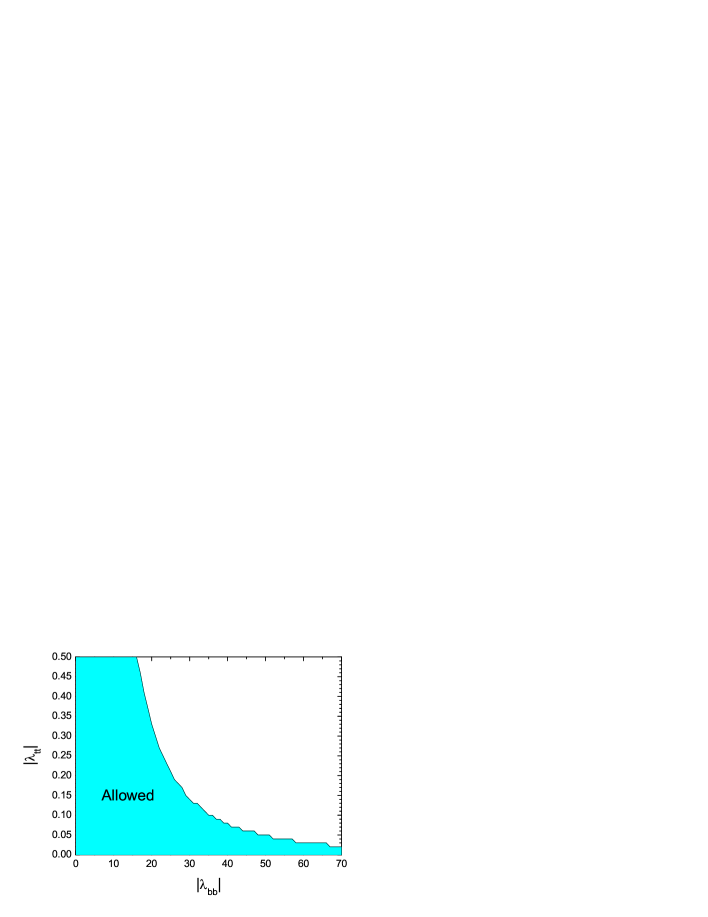
In hll we calculated the constraint on $|\lambda_{bb}|$ and $|\lambda_{tt}|$ due to the experimental upper bound of $Br(B_{s}\rightarrow\mu^{+}\mu^{-})$ which is pdg2003

$$B_{r}(B_{s}\rightarrow\mu^{+}\mu^{-})<2.0\times 10^{-6}(CL=90\%)$$ (31)

Recently, the Ref. cdf04 gave the new bound of $Br(B_{s}\rightarrow\mu^{+}\mu^{-})$ which reads

$$B_{r}(B_{s}\rightarrow\mu^{+}\mu^{-})<5.8\times 10^{-7}(CL=90\%)$$ (32)

With the updating upper bound of $Br(B_{s}\rightarrow\mu^{+}\mu^{-})$, we recalculate the constraint on $|\lambda_{bb}|$ and $|\lambda_{tt}|$ and the result is shown in Fig.1. The cyan region is allowed by the new experimental bound of $Br(B_{s}\rightarrow\mu^{+}\mu^{-})$. Comparing with the Fig.3 in Ref. hll , we find that the new bound gives a more stringent constraint on the values of $|\lambda_{bb}|$ and $|\lambda_{tt}|$, as expected.

It is shown in Ref. bck that the strictest constraints on $\lambda_{bb}$ and $\lambda_{tt}$ come from $B\rightarrow X_{s}\gamma$ and the neutron electric dipole moment (NEDM). Considering the theoretical uncertainties, we take $2.0\times 10^{-4}<{\rm Br}(B\to X_{s}\gamma)<4.5\times 10^{-4}$, as generally analyzed in literatures. The NEDM can be expressed as

$$d^{g}_{n}=10^{-25}\hbox{e$\cdot$cm}\ \hbox{Im}(\lambda_{tt}\lambda_{bb})\left({\alpha(m_{n})\over\alpha(\mu)}\right)^{1\over 2}\left({\xi_{g}\over 0.1}\right)H\left({m_{t}^{2}\over M^{2}_{H^{\pm}}}\right)$$ (33)

with

$$H(y)={3\over 2}{y\over(1-y)^{2}}\left(y-3-{2\log y\over 1-y}\right)$$ (34)

Here the parameter $\xi_{g}$ has been estimated and has different values obtained by different methods: 0.03, 0.07 and 1, which is due to the hadronic uncertainty bck . Using the result in Ref.bck , considering the uncertainty of $\xi_{g}$ and finding the maximally possible $|\lambda_{bb}\lambda_{tt}|$ which satisfies the experimental constraints, and requiring that the charged Higgs boson is not too heavy (say, $m_{H^{\pm}}<250GeV$) and the phase of $\lambda_{bb}\lambda_{tt}$ is not too limited, it follows that $|\lambda_{bb}\lambda_{tt}|\sim 3$.

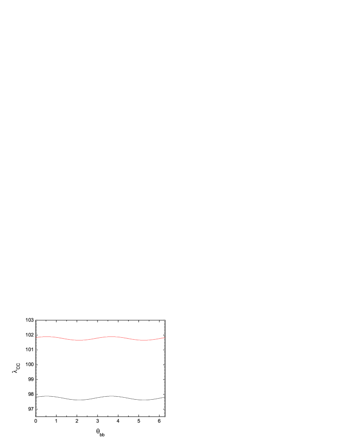
From the well measured physical observable $\Delta M_{B_{d}}$ and using the values of $|\lambda_{bb}|$ and $|\lambda_{tt}|$ analyzed above, one can get the constraint on $|\lambda_{cc}|$ in the model III. In Fig.2, we show the correlation between $|\lambda_{cc}|$ and $\theta_{bb}$ ($\theta_{ii}$ is the phase of $\lambda_{ii}$) for $\theta_{bb}+\theta_{tt}=\pi/2$ due to the constraint from $\Delta M_{B_{d}}$ within the $1\sigma$ deviation (i.e., $\Delta M_{B_{d}}=0.502\pm 0.007ps^{-1}$). One can see from the figure that the constraint on $|\lambda_{cc}|$ is very stringent and the dependence of $|\lambda_{cc}|$ on $\theta_{bb}$ is weak. We have also carried out the calculations for different values of $\theta_{bb}+\theta_{tt}$ in the allowed range and the results are similar, i.e., the dependence of $|\lambda_{cc}|$ on both $\theta_{bb}$ and $\theta_{tt}$ is weak.

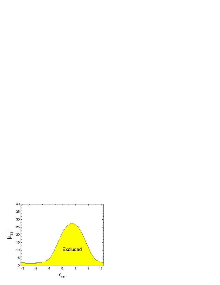
With the experimental lower bound of $\Delta M_{B_{s}}$, i.e., $\Delta M_{B_{s}}>14.4ps^{-1}$, we can draw the lower bound on $|\lambda_{ss}|$. Fig.3 is the contour plot of $|\lambda_{ss}|$ versus $\theta_{ss}$ for fixed $|\lambda_{tt}|$, $|\lambda_{bb}|$ and $|\lambda_{cc}|$ which satisfied the constraints from $B_{d}-\bar{B}_{d}$ mixing , $\Gamma(b\to s\gamma)$, $\Gamma(b\to c\tau\bar{\nu}_{\tau})$, $\rho_{0}$, $R_{b}$ and the electric dipole moment of neutron. The yellow area is excluded by the measured experimental bound. Above the yellow region, all the values of $|\lambda_{ss}|$ are allowed. We hope that the future B factory can make precise measurements of $\Delta M_{B_{s}}$, consequently, the more stringent constraints on the free parameters in the model III can be obtained.

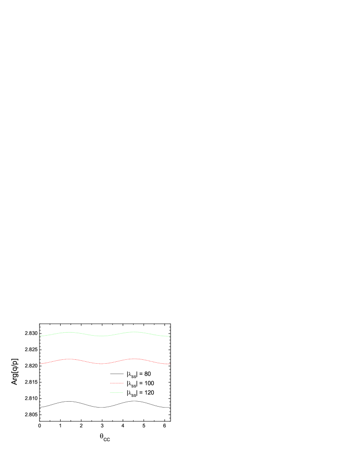
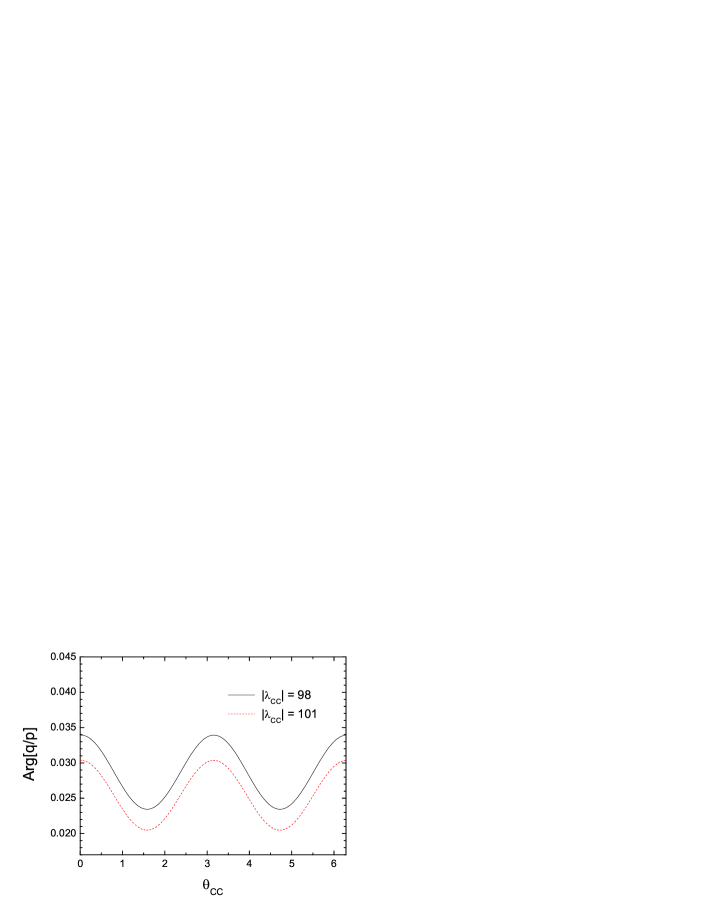
Using the values of parameters obtained by analyzing above, we calculate the new contribution to the ratio $q/p$. The Figs. 4 and 5 are devoted to $Arg[(q/p)_{n}]$ which denotes the new contribution to the phase of $q/p$ versus $\theta_{cc}$ for $B_{s}$ and $B_{d}$ systems respectively. As for the $B_{s}$ system, in Fig.4, we show the $Arg[(q/p)_{n}]$ dependence on $\theta_{cc}$ for fixed $|\lambda_{cc}|=100$ and for $|\lambda_{ss}|=80$ (solid curve), 100 (short-dashed curve) and 120 (dotted curve) respectively. From the figure we find $Arg[(q/p)_{n}]$ increases with $|\lambda_{ss}|$ increasing. In particular, $Arg[(q/p)_{n}]$ is large enough to give significant effects on CP violation in the neutral $B_{s}$ system. In Fig.5, for the $B_{d}$ system, the solid curve corresponds $|\lambda_{cc}|=98$ and the dotted one corresponds $|\lambda_{cc}|=101$. We find the phase of $(q/p)_{n}$ is very small, which verifies the expectation in Ref.hll , and consequently in agreement with the measurements of the time dependent CP asymmetry $S_{J/\psi K}$ in $B\to J/\psi K_{S}$. In contrast with the case of $B_{s}$, $Arg[(q/p)_{n}]$ decreases while $|\lambda_{cc}|$ increasing.

V Conclusions

In summary, we have calculated the new physics contributions to the neutral B meson mass splitting $\Delta M_{B_{q}}$ (q=d, s) at the NLO level in the model III 2HDM, while taking into account the new CP violating complex phases involved Higgs bosons and fermions coupling. By comparing the theoretical predictions with the high accuracy data as well as other relevant data, we have drawn the constraints on the free parameters of model III. Moreover, by using the constrained parameters we calculated the corrections to the ratio $q/p$. It is found that the phase of $(q/p)_{n}$ for $B_{d}$ which is due to the new contributions is very small and consequently in agreement with the measurements of the time dependent CP asymmetry $S_{J/\psi K}$ in $B\to J/\psi K_{S}$. On the contrary, the phase of $(q/p)_{n}$ for $B_{s}$ is large enough to give significant effects on CP violation in the neutral $B_{s}$ system.

Appendix

The Passarino-Veltman one-loop four-point functions with zero external momenta are defined as

$$\int\frac{d^{4}q}{i\pi^{2}}\frac{1}{(q^{2}-m_{0}^{2})(q^{2}-m_{1}^{2})(q^{2}-m_{2}^{2})(q^{2}-m_{3}^{2})}=D_{0}(m_{0}^{2},m_{1}^{2},m_{2}^{2},m_{3}^{2})$$ (35)

$$\int\frac{d^{4}q}{i\pi^{2}}\frac{q_{\mu}q_{\nu}}{(q^{2}-m_{0}^{2})(q^{2}-m_{1}^{2})(q^{2}-m_{2}^{2})(q^{2}-m_{3}^{2})}=g_{\mu\nu}D_{00}(m_{0}^{2},m_{1}^{2},m_{2}^{2},m_{3}^{2})$$ (36)

where

$$D_{0}(m^{2}_{0},m^{2}_{1},m^{2}_{3},m^{2}_{3})=\frac{1}{6}\frac{1}{m^{4}_{3}}f_{d0}(x,y,z)\hskip 34.1433ptx=\frac{m^{2}_{0}}{m^{2}_{3}},y=\frac{m^{2}_{1}}{m^{2}_{3}},z=\frac{m^{2}_{2}}{m^{2}_{3}}$$ (37)

$$D_{00}(m^{2}_{0},m^{2}_{1},m^{2}_{2},m^{2}_{3})=-\frac{1}{12}\frac{1}{m^{2}_{3}}f_{d00}(x,y,z)\hskip 28.45274ptx=\frac{m^{2}_{0}}{m^{2}_{3}},y=\frac{m^{2}_{1}}{m^{2}_{3}},z=\frac{m^{2}_{2}}{m^{2}_{3}}$$ (38)

with

$$f_{d0}(x,y,z) = 6\left[\frac{x\ln x}{(1-x)(x-y)(x-z)}+\frac{y\ln y}{(1-y)(y-x)(y-z)}\right.\$$ (39)

$$+ \left.\frac{z\ln z}{(1-z)(z-x)(z-y)}\right]$$

$$f_{d00}(x,y,z) = -3\left[\frac{x^{2}\ln x}{(1-x)(x-y)(x-z)}+\frac{y^{2}\ln y}{(1-y)(y-x)(y-z)}\right.\$$ (40)

$$+ \left.\frac{z^{2}\ln z}{(1-z)(z-x)(z-y)}\right]$$

Figure 1: The constraint on $|\lambda_{bb}|$ and $|\lambda_{tt}|$ due to the new experimental upper bound on $Br(B_{s}\rightarrow\mu^{+}\mu^{-})$ which reads $Br(B_{s}\rightarrow\mu^{+}\mu^{-})<5.8\times 10^{-7}(CL=90\%)$.

Figure 2: The constraint on $|\lambda_{cc}|$ due to the measured $\Delta M_{B_{d}}$ within $1\sigma$ deviation.

Figure 3: The constraint on $|\lambda_{ss}|$ due to the lower experimental bound on $\Delta M_{B_{s}}$.

Figure 4: $Arg[(q/p)_{n}]$ for $B_{s}$ system versus the CP violating phase $\theta_{cc}$, for $|\lambda_{cc}|=100$. The solid curve stands for $|\lambda_{ss}|=80$, the short-dashed curve stands for $|\lambda_{ss}|=100$ and the dotted curve stands for $|\lambda_{ss}|=120$ respectively.

Figure 5: $Arg[(q/p)_{n}]$ for $B_{d}$ system versus CP violating phase $\theta_{cc}$ for $|\lambda_{cc}|=98$ (the solid curve) and for $|\lambda_{cc}|=101$ (the dotted curve) respectively.

References

• (1) The BaBar Collaboration, B. Aubert et al., Phys. Rev. Lett. 89, 201802 (2002).
• (2) The Belle Collaboration, K. Abe et al., Phys. Rev. D 66, 071102 (2002).
• (3) T.ย Affoler et al., Phys. Rev. D 61, 072005 (2000).
• (4) Y. Nir, Lectures presented at the Twentieth Annual Summer Institute on Particle Physics, SLAC, Stanford, California 94309, July 13-24, 1992.
• (5) Y. Nir, hep-ph/9911321 (IASSNS-HEP-99-96).
• (6) Particle Data Group, K.ย Hagiwara et al., Phys. Rev. D 66, 010001 (2002) and 2003 partial update for edition 2004 (URL: http://pdg.lbl.gov).
• (7) The LEP B oscillation Working Group, http://www.cern.ch/LEPBOSC/.
• (8) L.F.ย Abbot, P.ย Sikivie, and M.B.ย Wise, Phys. Rev. D , 21, 1393 (1980); S.L.Glashow and E.E.ย Jenkins, Phys. Lett. B 196, 233(1987); G.G.ย Athanasiu, P.J.ย Franzini, and F.J.ย Gilman, Phys. Rev. D 32, 3010 (1985); C.Q.ย Geng and J.N.ย Ng, Phys. Rev. D 32, 3010 (1985);
• (9) A.J.ย Buras, M.Jamin, and P.H.Weisz, Nucl. Phys. B 347, 491 (1990).
• (10) J.ย Urban, F.ย Krauss, U.ย Jentschura, and G.ย Soff, Nucl. Phys. B 523, 40 (1998).
• (11) A.ย Grant, Phys. Rev. D 51, 207 (1995).
• (12) D.ย Atwood, L.ย Reina and A.ย Soni, Phys. Rev. D 55, 3156 (1997).
• (13) D. Bowser-Chao, K. Cheung, and W.-Y. Keung, Phys. Rev. D 59, 115006 (1999).
• (14) Z.J. Xiao, L.B. Guo, Phys. Rev. D 69, 014002 (2004).
• (15) S.ย Glashow and S.ย Weinberg, Phys. Rev. D 15, 1958 (1977).
• (16) J.F.ย Gunion, H.E.ย Haber, G.ย Kane, and S.ย Dawson, The Higgs Hunterโ€™s Guide,Addison Wesley, Redwood-City (1990), and references therein.
• (17) T.P. Cheng and M. Sher, Phys. Rev. D 35, 3484 (1987); M. Sher and Y. Yuan, Phys. Rev. D 44, 1461 (1991).
• (18) W.S. Hou, Phys. Lett. B296, 179 (1992); A. Antaramian, L.J. Hall, and A. Rasin, Phys. Rev. Lett. 69, 1871 (1992); L.J. Hall and S. Weinberg, Phys. Rev. D 48, 979 (1993); M.J. Savage, Phys. Lett. B 266, 135 (1991); L. Wolfenstein and Y.L. Wu, Phys. Rev. Lett. 73, 1762 (1994); D.ย Chang, W.S.ย Hou, and W.Y.ย Keung, Phys. Rev. D 48, 217 (1993); D.ย Atwood, L.ย Reina and A.ย Soni, Phys. Rev. Lett. 75, 3800 (1995).
• (19) Y.-B. Dai, C.-H. Huang, J.-T. Li, W.-J. Li, Phys. Rev. D 67, 096007 (2003).
• (20) J. Rosiek, Phys. Rev. D 41, 3464 (1990), Erratum hep-ph/9511250.
• (21) T. Inami, C. Lim, Prog.Theor.Phys. 65, 297 (1981).
• (22) A. J. Buras, P. H. Chankowski, J. Rosiek, and L. Slawianowska, Nucl.Phys. B 619, 434 (2001).
• (23) D.ย Beฤ‡ireviฤ‡, M.ย Ciuchini, E.ย Franco, V.ย Gimรฉnez, G.ย Martinelli, A.ย Masiero, M.ย Papinutto, J.ย Reyes and L.ย Silvestrini, Nucl. Phys. B 634, 105 (2002).
• (24) G.ย Buchalla, A.J.ย Buras, and M.E.ย Lautenbacher, Rev. Mod. Phys. 68, 1125 (1996).
• (25) D.ย Beฤ‡ireviฤ‡ et al., Nucl. Phys. Proc. Suppl. 106, 385 (2002); JHEP 0204, 025 (2002).
• (26) H.ย Wittig, Invited talk at Int. Europhysics Conf. on High Energy Physics, EPS-HEP2003, 17-23 July 2003, Aachen, Germany, arXiv: hep-ph/0310329.
• (27) D.ย Beฤ‡ireviฤ‡, XXXVIII Rencontres de Moriond, Les Arcs, France, (2003).
• (28) M.ย Battaglia et al., Proceedings of the First Workshop on the CKM Unitary Triangle, CERN 13-16 February 2002, arXiv: hep-ph/0304132.
• (29) M.ย Beneke, A.ย Lenz, J. Phys. G 27, 1219 (2001).
• (30) D.ย Acosta et al., CDF Collaboration, arXiv: hep-ex/0403032.
Refer to caption
Figure 1: The constraint on |ฮปbโ€‹b|subscript๐œ†๐‘๐‘|\lambda_{bb}| and |ฮปtโ€‹t|subscript๐œ†๐‘ก๐‘ก|\lambda_{tt}| due to the new experimental upper bound on Bโ€‹rโ€‹(Bsโ†’ฮผ+โ€‹ฮผโˆ’)๐ต๐‘Ÿโ†’subscript๐ต๐‘ superscript๐œ‡superscript๐œ‡Br(B_{s}\rightarrow\mu^{+}\mu^{-}) which reads Bโ€‹rโ€‹(Bsโ†’ฮผ+โ€‹ฮผโˆ’)<5.8ร—10โˆ’7โ€‹(Cโ€‹L=90%)๐ต๐‘Ÿโ†’subscript๐ต๐‘ superscript๐œ‡superscript๐œ‡5.8superscript107๐ถ๐ฟpercent90Br(B_{s}\rightarrow\mu^{+}\mu^{-})<5.8\times 10^{-7}(CL=90\%).
Figure 2: The constraint on |ฮปcโ€‹c|subscript๐œ†๐‘๐‘|\lambda_{cc}| due to the measured ฮ”โ€‹MBdฮ”subscript๐‘€subscript๐ต๐‘‘\Delta M_{B_{d}} within 1โ€‹ฯƒ1๐œŽ1\sigma deviation.
Figure 3: The constraint on |ฮปsโ€‹s|subscript๐œ†๐‘ ๐‘ |\lambda_{ss}| due to the lower experimental bound on ฮ”โ€‹MBsฮ”subscript๐‘€subscript๐ต๐‘ \Delta M_{B_{s}}.
Figure 4: Aโ€‹rโ€‹gโ€‹[(q/p)n]๐ด๐‘Ÿ๐‘”delimited-[]subscript๐‘ž๐‘๐‘›Arg[(q/p)_{n}] for Bssubscript๐ต๐‘ B_{s} system versus the CP violating phase ฮธcโ€‹csubscript๐œƒ๐‘๐‘\theta_{cc}, for |ฮปcโ€‹c|=100subscript๐œ†๐‘๐‘100|\lambda_{cc}|=100. The solid curve stands for |ฮปsโ€‹s|=80subscript๐œ†๐‘ ๐‘ 80|\lambda_{ss}|=80, the short-dashed curve stands for |ฮปsโ€‹s|=100subscript๐œ†๐‘ ๐‘ 100|\lambda_{ss}|=100 and the dotted curve stands for |ฮปsโ€‹s|=120subscript๐œ†๐‘ ๐‘ 120|\lambda_{ss}|=120 respectively.
Figure 5: Aโ€‹rโ€‹gโ€‹[(q/p)n]๐ด๐‘Ÿ๐‘”delimited-[]subscript๐‘ž๐‘๐‘›Arg[(q/p)_{n}] for Bdsubscript๐ต๐‘‘B_{d} system versus CP violating phase ฮธcโ€‹csubscript๐œƒ๐‘๐‘\theta_{cc} for |ฮปcโ€‹c|=98subscript๐œ†๐‘๐‘98|\lambda_{cc}|=98 (the solid curve) and for |ฮปcโ€‹c|=101subscript๐œ†๐‘๐‘101|\lambda_{cc}|=101 (the dotted curve) respectively.