The neutrino charge radius in the presence of fermion masses

Abstract

We show how the crucial gauge cancellations leading to a physical definition of the neutrino charge radius persist in the presence of non-vanishing fermion masses. An explicit one-loop calculation demonstrates that, as happens in the massless case, the pinch technique rearrangement of the Feynman amplitudes, together with the judicious exploitation of the fundamental current relation $J_{\alpha}^{(3)}=2(J_{Z}+\sin\theta_{\rm w}^{2}J_{\gamma})_{\alpha}$, leads to a completely gauge independent definition of the effective neutrino charge radius. Using the formalism of the Nielsen identities it is further proved that the same cancellation mechanism operates unaltered to all orders in perturbation theory.

I Introduction

It is well-known that, even though within the Standard Model (SM) the photon ($A$) does not interact with the neutrino ($\nu$) at tree-level, an effective photon-neutrino vertex ${\Gamma}^{\mu}_{A\nu\bar{\nu}}$ is generated through one-loop radiative corrections, giving rise to a non-zero neutrino charge radius (NCR) Bernstein:jp . Traditionally (and, of course, rather heuristically) the NCR has been interpreted as a measure of the “size” of the neutrino $\nu$ when probed electromagnetically, owing to its classical definition footnote (in the static limit) as the second moment of the spatial neutrino charge density $\rho_{\nu}(\bf{r})$, i.e. $\big{<}r^{2}_{\nu}\,\big{>}=\int\!d{\bf{r}}\,r^{2}\rho_{\nu}({\bf{r}})$. However, the direct calculation of this quantity has been faced with serious complications Lucio:1984mg which, in turn, can be traced back to the fact that in non-Abelian gauge theories off-shell Green’s functions depend in general explicitly on the gauge-fixing parameter. In the popular renormalizable ($R_{\xi}$) gauges, for example, the electromagnetic form-factor $F_{1}$ depends explicitly on gauge-fixing parameter $\xi$ in a prohibiting way. Specifically, even though in the static limit of zero momentum transfer, $q^{2}\to 0$, the form-factor $F(q^{2},\xi)$ becomes independent of $\xi$, its first derivative with respect to $q^{2}$, which corresponds to the definition of the NCR, namely $\big{<}r^{2}_{\nu}\,\big{>}=-\,6\,(dF/dq^{2})_{q^{2}=0}$  , continues to depend on it. Similar (and some times worse) problems occur in the context of other gauges (e.g. the unitary gauge).

One way out of this difficulty is to identify a modified vertex-like amplitude, which could lead to a consistent definition of the electromagnetic form factor and the corresponding NCR. The basic idea is to exploit the fact that the full one-loop $S$-matrix element describing the interaction between a neutrino with a charged particle is gauge-independent, and try to rearrange the Feynman graphs contributing to this scattering amplitude in such a way as to find a vertex-like combination that would satisfy all desirable properties. What became gradually clear over the years was that, for reaching a physical definition for the NCR, in addition to gauge-independence, a plethora of important physical constraints need be satisfied. For example, one should not enforce gauge-independence at the expense of introducing target-dependence. Therefore, a definite guiding-principle is needed, allowing for the systematic construction of physical sub-amplitudes with definite kinematic structure (i.e., self-energies, vertices, boxes).

The field-theoretical methodology allowing this meaningful rearrangement of the perturbative expansion is that of the pinch technique (PT) Cornwall:1982zr . The PT is a diagrammatic method which exploits the underlying symmetries encoded in a physical amplitude, such as an $S$-matrix element, in order to construct effective Green’s functions with special properties. In the context of the NCR, the basic observation Bernabeu:2000hf is that the gauge-dependent parts of the conventional $A^{*}\nu\nu$, to which one would naively associate the (gauge-dependent) NCR, communicate and eventually cancel algebraically against analogous contributions concealed inside the $Z^{*}\nu\nu$ vertex, the self-energy graphs, and the box-diagrams (if there are boxes in the process), before any integration over the virtual momenta is carried out. For example, due to rearrangements produced through the systematic triggering of elementary Ward identities, the gauge-dependent contributions coming from boxes are not box-like, but self-energy-like or vertex-like; it is only those latter contributions that need be included in the definition of the new, effective $\widehat{A}^{*}\nu\nu$ vertex.

The new one-loop proper three-point function satisfies the following properties Bernabeu:2002nw ; Bernabeu:2002pd ; Papavassiliou:2003rx : (i) is independent of the gauge-fixing parameter ($\xi$); (ii) is ultra-violet finite; (iii) satisfies a QED-like Ward-identity; (iv) captures all that is coupled to a genuine $(1/q^{2})$ photon propagator, before integrating over the virtual momenta; (v) couples electromagnetically to the target; (vi) does not depend on the $SU(2)\times U(1)$ quantum numbers of the target-particles used; (vii) has a non-trivial dependence on the mass $m_{i}$ of the charged iso-spin partner $f_{i}$ of the neutrino in question; (viii) contains only physical thresholds; (ix) satisfies unitarity and analyticity; (x) can be extracted from experiments.
Notice in particular that the properties from (iv) to (vi) ensure that the quantity constructed is a genuine photon vertex, uniquely defined in the sense that it is independent of using either weak iso-scalar sources (coupled to the $B$-field) or weak iso-vector sources (coupled to $W^{0}$), or any other charged combination. As for property (x), the NCR defined through this procedure may be extracted from experiment, at least in principle, by expressing a set of experimental electron-neutrino cross-sections in terms of the finite NCR and two additional gauge- and renormalization-group-invariant quantities, corresponding to the electroweak effective charge and mixing angle Bernabeu:2002nw ; Bernabeu:2002pd .

Given the progress achieved with the above properties for the NCR, it is important to address some of the remaining open theoretical issues. To begin with, in the construction presented in Bernabeu:2000hf it has been tacitly assumed that the mass of the iso-doublet partner of the neutrino under consideration vanishes (except when needed for controlling infra-red divergences). That should be a acceptable approximation, given the fact that the fermion masses are naturally suppressed numerically, relative to the relevant physical scale, i.e., the mass of the $W$-boson, provided that the neglected pieces form themselves a gauge-independent sub-set. As has been pointed out Fujikawa:2003ww , when computing the conventional vertex (that is, before applying any PT rearrangements) in the $R_{\xi}$ gauges and keeping the fermion masses non-zero, a gauge-dependent term survives, which, in fact, diverges at $\xi=0$. It is therefore an indispensable exercise to verify that the PT procedure in the presence of masses indeed identifies precisely the contributions which will cancell such pathological terms, exactly as happens in the massless case, without any additional assumptions. In this article we will undertake this task and demonstrate through an explicit calculation how the (vertex-like) gauge-dependent contribution proportional to the fermion masses cancel partially against similar gauge-dependent contributions stemming from graphs containing would-be Goldstone bosons, and partially against vertex-like contributions concealed inside box-graphs, exactly as dictated by the well-defined PT procedure.

In addition, the constructions related to the NCR have thus far been solely restricted to the one-loop level. Clearly, it is important to demonstrate that the crucial cancellations and non-trivial rearrangements operating at one-loop persist and can be generalized to all orders. In this article we demonstrate that the pertinent gauge-cancellations take place through precisely the same mechanism as at one-loop, by resorting to the powerful formalism of the Nielsen identities (NIs) Nielsen:1975fs . These identities control in a concise, completely algebraic way, the gauge-dependences of individual Green’s functions (such as the off-shell photon-neutrino vertex ${\Gamma}^{\mu}_{A\nu\bar{\nu}}$ in question), and allow for an all-order demonstration of gauge-cancellations between various Green’s functions, when the latter are combined to form ostensibly gauge-invariant quantities, such as $S$-matrix elements. In the present paper, using the corresponding NIs, we will show that the gauge-dependence of the vertex ${\Gamma}_{A_{\mu}\nu\bar{\nu}}$ has precisely the form needed for cancelling against analogous gauge-dependent vertex-like contributions from the boxes, employing nothing more than the fundamental current relation (see, for example, the sixth reference in  Lucio:1984mg )

$$J_{\alpha}^{(3)}=2(J_{Z}+s_{\rm w}^{2}J_{\gamma})_{\alpha},$$ (1)

with $s_{\rm w}\equiv\sin\theta_{\rm w}$, and $J_{\alpha}^{(3)}$ the third iso-triplet current of $SU(2)_{L}$.

The paper is organized as follows: In Section II we present an explicit one-loop proof of the relevant gauge cancellations in the presence of non-vanishing fermion masses. The upshot of this construction is to demonstrate that the fermion masses do not distort in the least the crucial $s$-$t$ channel cancellations characteristic of the PT, and that, at the end of the cancellation procedure, a completely gauge-independent NCR emerges. In Section III we present a general all-order proof of the same gauge-cancellations, by means of the NIs. Finally, in Section IV, we present our conclusions.

II Gauge cancellations in the presence of fermion masses

In this section we go over the fundamental cancellation mechanism, and outline its basic ingredients. In particular, we emphasize the topological modifications induced on Feynman diagrams due to the presence of longitudinal momenta, the rôle of the current operator identity in implementing the gauge cancellations, and explain qualitatively the modifications induced when the fermion masses are turned on. Then, we carry out an explicit one-loop calculation in the presence of non-vanishing fermion masses, and demonstrate the precise cancellations of massive gauge-dependent terms. In doing so we will show that no additional theoretical input or assumptions are needed, whatsoever.

II.1 General considerations

The topological modifications, which allow the communication between kinematically distinct graphs (enforcing eventually the cancellation of the gauge dependent pieces), are produced when elementary Ward identities are triggered by the virtual longitudinal momenta ($k$) inside Feynman diagrams, furnishing inverse propagators Cornwall:1982zr . The longitudinal momenta appearing in the $S$-matrix element of $f\nu\to f\nu$ originate from the tree-level gauge-boson propagators and tri-linear gauge-boson vertices appearing inside loops. In particular, in the $R_{\xi}$-scheme the gauge-boson propagators have the general form

$$\Delta^{\mu\nu}_{i}(k)=-i\Bigg{[}g^{\mu\nu}-\frac{(1-\xi_{i})k^{\mu}k^{\nu}}{k^{2}-\xi_{i}M_{i}^{2}}\Bigg{]}D_{i}(k)$$ (2)

with

$$D_{i}(k)=(k^{2}-M_{i}^{2})^{-1}$$ (3)

where $i=W,V$ with $V=Z,A$ and $M^{2}_{A}=0$; $k$ denotes the virtual four-momentum circulating in the loop. Clearly, in the case of $\Delta^{\mu\nu}_{i}(k)$ the longitudinal momenta are those proportional to $(1-\xi_{i})$. The longitudinal terms arising from the tri-linear vertex may be identified by splitting its Lorentz structure $\Gamma_{\alpha\mu\nu}(q,-k,k-q)$ appearing inside the one-loop diagrams (where $q$ denotes the physical four-momentum entering into the vertex, see Section II.3) into two parts Cornwall:1976ii :

$$\Gamma_{\alpha\mu\nu}(q,-k,k-q) = (k+q)_{\nu}g_{\alpha\mu}+(q-2k)_{\alpha}g_{\mu\nu}(k-2q)_{\mu}g_{\alpha\nu}$$ (4)

$$= \Gamma_{\alpha\mu\nu}^{\rm F}+\Gamma_{\alpha\mu\nu}^{\rm P}\,,$$

where

$$\Gamma_{\alpha\mu\nu}^{\rm F} = (q-2k)_{\alpha}g_{\mu\nu}+2q_{\nu}g_{\alpha\mu}-2q_{\mu}g_{\alpha\nu},$$

$$\Gamma_{\alpha\mu\nu}^{\rm P} = (k-q)_{\nu}g_{\alpha\mu}+k_{\mu}g_{\alpha\nu}.$$ (5)

The first term in $\Gamma_{\alpha\mu\nu}^{\rm F}$ is a convective vertex describing the coupling of a vector boson to a scalar field, whereas the other two terms originate from spin or magnetic moment. The above decomposition assigns a special rôle to the $q$-leg, and allows $\Gamma_{\alpha\mu\nu}^{\rm F}$ to satisfy the Ward identity

$$q^{\alpha}\Gamma_{\alpha\mu\nu}^{\rm F}=(k-q)^{2}g_{\mu\nu}-k^{2}g_{\mu\nu}\,,$$ (6)

The relevant Ward identities triggered by the longitudinal momenta identified above, are then two. The first one reads

$$k/P_{\!\scriptscriptstyle{L}} = (k/+p/)P_{\!\scriptscriptstyle{L}}-P_{\!\scriptscriptstyle{R}}\not\!p$$ (7)

$$= S_{f^{\prime}}^{-1}(k/+p/)P_{\!\scriptscriptstyle{L}}-P_{R}S_{f}^{-1}(p/)+m_{f^{\prime}}P_{\!\scriptscriptstyle{L}}-m_{f}P_{\!\scriptscriptstyle{R}},$$

where $P_{R(L)}=[1+(-)\gamma_{5}]/2$ is the chirality projection operator and $iS_{f}$ is the tree-level propagator of the fermion $f$; $f^{\prime}$ is the iso-doublet partner of the external fermion $f$. (Alternatively, one may adopt the formulation of the PT in terms of equal-time commutators of currents Degrassi:1992ue ). The second Ward identity reads

$$(k-q)^{\nu}\Gamma_{\alpha\mu\nu}(q,-k,k-q)=\bigg{[}k^{2}g_{\alpha\mu}-k_{\alpha}k_{\mu}\bigg{]}-\bigg{[}q^{2}g_{\alpha\mu}-q_{\alpha}q_{\mu}\bigg{]},$$ (8)

together with the Bose-symmetric one, when contracting with $k^{\mu}$ instead of $(k-q)^{\nu}$.

The appearance of inverse propagators leads (through the pinching out of the corresponding internal propagators) to $\xi$-dependent contributions which are topologically distinct from those of their parent Feynman graph. Because of that, all $\xi$-dependent parts violate one or more of the properties (i)–(x) listed in the Introduction. In particular, if $m_{i}=0$ the gauge-dependent parts are purely propagator-like, i.e., they violate (vi), whereas if $m_{i}\neq 0$ they are either propagator-like (hence violating (vi)), or they are multiplied by a factor $q^{2}$, i.e., they effectively violate (i).

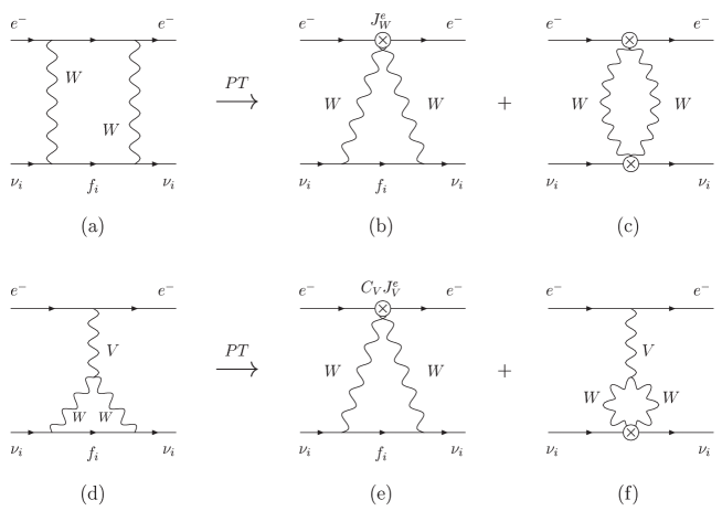
Figure 1: The general topology of the relevant gauge-dependent contributions in the presence of non-vanishing fermion masses. The contributions (b) and (e) are proportional to $m_{i}$. If the target-fermions are (massless) right-handed fermions, the entire first column of the right-hand side vanishes.

Before entering into the explicit proof, it is instructive to briefly sketch how the cancellation of the gauge-dependent terms proceeds:

• The $\xi$-dependent propagator-like (universal, or equivalently flavor-independent) parts [shown in (c) and (f)] cancel against corresponding $\xi$-dependent contributions from the conventional self-energy graphs (not shown), for every neutrino flavor. The emerging gauge-independent effective self-energies form renormalization-group-invariant quantities (electroweak effective charges) exactly as in QED.

• The vertex-like (flavor-dependent) parts [shown in (b) and (e)] are proportional to $m_{i}$; they stem from the mass-terms appearing on the right-hand side of Eq.(7). The particular topology of the graph (e) (i.e., contact-type interaction) arises because the $\xi$-dependent part coming from the $A^{*}\nu\nu$ vertex are proportional to $q^{2}$, whereas those from the $Z^{*}\nu\nu$ vertex are proportional to $(q^{2}-M_{Z}^{2})$ [this is essentially due to the Ward identity of Eq.(8)]. On the other hand, graph (b) has this form due to Eq.(7). The topological form of these graphs is crucial for the cancellation, because it allows parts of the three (originally distinct) graphs to “talk” to each other. The next step is to recognize that, the current structures of the contact-like interactions are such that the total sum of the two pieces is zero, i.e.,

  $$({\rm b})+\sum_{V}({\rm e})=0.$$ (9)

  This final cancellation is not accidental, but a direct consequence of the current operator identity of Eq.(1).

We emphasize that (see also property (vi) in the Introduction) the definition and value of NCR should be independent of the charged probe used. If one were to use as a probe massless right-handed electrons, $e_{R}$, there would be no boxes containing $W$-bosons involved in the gauge cancellations, $({\rm b})=0$; however in this case the current structures of diagrams $({\rm e})$ get modified in such a way that now $\sum_{V}({\rm e})=0$ (see Bernabeu:2000hf and below for a detailed discussion).

II.2 Review of the massless case

The massless case has been studied in detail in Bernabeu:2000hf ; Bernabeu:2002nw . For concreteness, we will focus on the same process considered there, namely the (one-loop) elastic scattering process $e(\ell_{1})\nu(p_{1})\to e(\ell_{2})\nu(p_{2})$, with the Mandelstam variables defined as $s=(\ell_{1}+p_{1})^{2}=(\ell_{2}+p_{2})^{2}$, $t=q^{2}=(p_{1}-p_{2})^{2}=(\ell_{2}-\ell_{1})^{2}$, $u=(\ell_{1}-p_{2})^{2}=(\ell_{2}-p_{1})^{2}$, and $s+t+u=0$. Notice that $\nu$ will be chosen to belong in a different iso-doublet than the target-electron (the muon neutrino $\nu_{\mu}$, for example), so that the crossed (charged) channel vanishes. According to the general PT algorithm, the one-loop amplitude for the above process may be reorganized into sub-amplitudes which have the same kinematic properties as self-energies, vertices, and boxes, and are at the same time completely independent of the gauge-fixing parameter. One of these sub-amplitudes will be identified with the one-loop effective photon-neutrino vertex.

What has been assumed in Bernabeu:2000hf ; Bernabeu:2002nw ; Bernabeu:2002pd when constructing the aforementioned vertex is that the masses of the fermions may be neglected when carrying out the various cancellations; in particular, one employs the Ward identity of Eq.(7), with the masses set to zero. In such a case, as mentioned earlier, all contributions stemming from longitudinal momenta are effectively propagator-like; they are combined with the normal self-energy graphs giving rise to two renormalization group invariant quantities, corresponding to the electroweak effective charge and the running mixing angle Hagiwara:1994pw .

After having removed all gauge-dependent propagator-like contributions, the remaining genuine one-loop vertex, to be denoted by $\widehat{\Gamma}_{A_{\mu}\nu_{i}\nu_{i}}$, is completely independent of the gauge-fixing parameter, and in addition satisfies a naive, QED-like Ward identity. As explained in detail in the literature, the final answer is given by the two graphs of Fig.2, where the Feynman gauge is used for all internal gauge-boson propagators, and the usual tree-level three-boson vertex $\Gamma_{\alpha\mu\nu}$ is replaced by $\Gamma_{\alpha\mu\nu}^{\rm F}$.

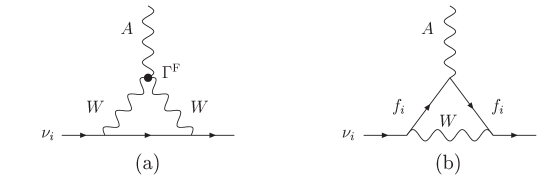
Figure 2: The diagrams contributing to the PT neutrino charge radius. Here $\Gamma^{\rm F}$ stands for the Feynman part of the tri-linear gauge-boson vertex, which is defined in Eq(4). Notice that the logarithmic term in the NCR expression of Eq.(11) originates entirely from the Abelian-like diagram (b).

It is straightforward to evaluate the two aforementioned vertex graphs; their sum gives a ultra-violet finite result, from which one can extract the dimension-less electromagnetic form-factor $\widehat{F}_{1}^{A}(q^{2})$. In particular, since $\widehat{F}_{1}^{A}(q^{2})$ is proportional to $q^{2}$, we may define the dimension-full form-factor $\widehat{F}_{\nu_{i}}(q^{2})$ as

$$\widehat{\Gamma}_{A_{\mu}\nu_{i}\bar{\nu}_{i}}=\widehat{F}_{1}^{A}(q^{2})\left[ie\gamma_{\mu}(1-\gamma_{5})\right]=q^{2}\widehat{F}_{\nu_{i}}(q^{2})\left[ie\gamma_{\mu}(1-\gamma_{5})\right],$$ (10)

from which the NCR is defined in the usual way as $\widehat{F}_{\nu_{i}}(0)=\frac{1}{6}\langle r^{2}_{\nu_{i}}\rangle$. We emphasize that, when taking the limit $q^{2}\to 0$, as dictated by the very definition of the NCR, $\widehat{F}_{\nu_{i}}(q^{2})$ is infrared divergent, unless the mass $m_{i}$ of the charged iso-doublet partner of the neutrino is kept non-zero. In particular, when $m_{i}\to 0$ a logarithmically divergent contribution emerges from the Abelian-like diagram of Fig.2(b). Thus, a non-zero mass must be eventually kept in the calculation of the final answer even in the “massless” case; evidently, the term “massless” refers to the fact that the massless version of the Ward identity has been employed, and mass terms appearing in the numerators (but not the denominators) of the corresponding Feynman graphs have been discarded.

The final answer is given by Bernabeu:2000hf

$$\big{<}r^{2}_{\nu_{i}}\,\big{>}=\frac{G_{\rm F}}{4\,{\sqrt{2}}\pi^{2}}\left[3-2\log\left(\frac{m_{i}^{2}}{M_{W}^{2}}\right)\right],\qquad i=e,\mu,\tau$$ (11)

where $G_{\rm F}=g_{\rm w}^{2}\sqrt{2}/8M_{W}^{2}$ is the Fermi constant and $g_{\rm w}=es_{\rm w}$ the $SU(2)$ gauge coupling. The numerical values obtained for the corresponding NCR of the three neutrino families Bernabeu:2002nw ; Bernabeu:2002pd are consistent with various bounds that have appeared in the literature Salati:1994tf .

II.3 The massive case: explicit one-loop calculation

After these introductory remarks, in the rest of this section we will show explicitly how the crucial cancellations, enforced by the PT through the tree-level Ward identities of the theory, continue to hold even when we relax the hypothesis of working with purely massless fermions. We will prove this in two different ways: first we will carry out an explicit one-loop calculation following simply the PT rules; second, we will re-do the analysis of gauge cancellations in their full generality, through the use of the so-called NIs, and show that the latter lead precisely to the same kind of rearrangements induced by the PT.

We consider again the same reference process $e(\ell_{1})\nu(p_{1})\to e(\ell_{2})\nu(p_{2})$ as before, and carry out the PT-rearrangement of the corresponding one-loop amplitude, but this time we will maintain throughout the calculation non-vanishing masses for the iso-doublet partner of the neutrino. In particular, we are interested in analyzing the box/vertex gauge cancellation in the case where we do not neglect the masses of the fermions propagating inside the loop, as originally done in Bernabeu:2002nw . Notice that the PT rearrangement, in addition to the quantities relevant for defining the NCR, will also give rise to one-loop vertices involving the off-shell photon or $Z$-boson and the target-fermions. In order to simplify the picture we will assume the target fermions to be massless. This has no bearing whatsoever on the cancellations taking place in the loops containing the massive iso-doublet partner of the neutrino; in any case, the assumption of massless target fermions will be relaxed later on, when presenting the treatment based on the NIs. Therefore, in what follows we will only focus on the PT terms contributing to the gauge cancellation of the photon-neutrino vertex $\Gamma^{(1)}_{A_{\mu}\nu\nu}$, and will not display terms involved in other parts of the full PT rearrangement, as for example in the construction of the one-loop vertex involving the target fermions. In addition, from the terms involved in the construction of the photon-neutrino vertex we will display only those proportional to the mass of the iso-doublet partner, since these are the new terms not considered in Bernabeu:2002nw .

Let us start by introducing the relevant tree-level photon and $Z$-boson vertices as

$$\Gamma^{(0)}_{V_{\mu}\bar{f}f}=ig_{\rm w}\gamma_{\mu}C_{V}^{f},\qquad\quad C_{V}^{f}=\left\{\begin{array}[]{ll}-s_{\rm w}Q_{f},&\quad{\rm if}\ \ V=A,\\ -\frac{1}{c_{\rm w}}\left[s_{\rm w}^{2}Q_{f}-T^{f}_{z}P_{L}\right],&\quad{\rm if}\ \ V=Z.\end{array}\right.$$ (12)

where $Q_{f}$ is the electric charge of the fermion $f$, $T^{f}_{z}$ represents the $z$ component of the weak iso-spin [which is $+(-)1/2$ for up (down)-type leptons], and $c_{\rm w}=\sqrt{1-s_{\rm w}^{2}}=M_{W}/M_{Z}$. In addition we define the following integrals

$$I_{1} = \{(k^{2}-M^{2}_{\scriptscriptstyle W})(k^{2}-\xi_{\scriptscriptstyle W}M^{2}_{\scriptscriptstyle W})[(k-q)^{2}-M^{2}_{\scriptscriptstyle W}]\}^{-1},$$

$$I^{\prime}_{1} = \{(k^{2}-M^{2}_{\scriptscriptstyle W})(k^{2}-\xi_{\scriptscriptstyle W}M^{2}_{\scriptscriptstyle W})[(k-q)^{2}-\xi_{\scriptscriptstyle W}M^{2}_{\scriptscriptstyle W}]\}^{-1},$$

$$I_{2} = \{(k^{2}-M^{2}_{\scriptscriptstyle W})[(k-q)^{2}-M^{2}_{\scriptscriptstyle W}][(k-q)^{2}-\xi_{\scriptscriptstyle W}M^{2}_{\scriptscriptstyle W}]\}^{-1},$$

$$I^{\prime}_{2} = \{(k^{2}-\xi_{\scriptscriptstyle W}M^{2}_{\scriptscriptstyle W})[(k-q)^{2}-M^{2}_{\scriptscriptstyle W}][(k-q)^{2}-\xi_{\scriptscriptstyle W}M^{2}_{\scriptscriptstyle W}]\}^{-1},$$

$$I_{3} = \{(k^{2}-M^{2}_{\scriptscriptstyle W})(k^{2}-\xi_{W}M^{2}_{\scriptscriptstyle W})[(k-q)^{2}-M^{2}_{\scriptscriptstyle W}][(k-q)^{2}-\xi_{\scriptscriptstyle W}M^{2}_{\scriptscriptstyle W}]\}^{-1},$$

$$I_{4} = \{(k^{2}-M^{2}_{\scriptscriptstyle W})[(k-q)^{2}-\xi_{\scriptscriptstyle W}M^{2}_{\scriptscriptstyle W}]\}^{-1},$$

$$I_{5} = \{(k^{2}-\xi_{\scriptscriptstyle W}M^{2}_{\scriptscriptstyle W})[(k-q)^{2}-M^{2}_{\scriptscriptstyle W}]\}^{-1},$$

$$I_{6} = \{(k^{2}-M^{2}_{\scriptscriptstyle W})(k^{2}-\xi_{\scriptscriptstyle W}M^{2}_{\scriptscriptstyle W})\}^{-1},$$ (13)

together with the characteristic PT structures

$$J = \bar{u}_{\nu}(p_{2})P_{\!\scriptscriptstyle{R}}\left[m_{\mu}^{2}S_{\mu}(k/+p/_{1})\right]P_{\!\scriptscriptstyle{L}}u_{\nu}(p_{1}),$$

$$J^{\alpha}_{1} = \bar{u}_{\nu}(p_{2})\gamma^{\alpha}P_{\!\scriptscriptstyle{L}}\left[m_{\mu}S_{\mu}(k/+p/_{1})\right]P_{\!\scriptscriptstyle{L}}u_{\nu}(p_{1}),$$

$$J^{\alpha}_{2} = \bar{u}_{\nu}(p_{2})P_{\!\scriptscriptstyle{R}}\left[m_{\mu}S_{\mu}(k/+p/_{1})\right]\gamma^{\alpha}P_{\!\scriptscriptstyle{L}}u_{\nu}(p_{1}).$$ (14)

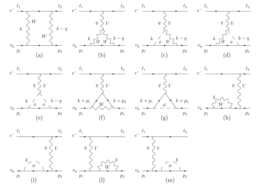
Figure 3: The diagrams contributing to the box/vertex PT cancellation for the case of massive propagating fermions.

Turning to individual diagrams, we first consider the box diagram $(a)$ of Fig.3, and isolate the PT vertex-like contributions; they will eventually cancel against the corresponding gauge dependent contributions of the vertices $\Gamma^{(1)}_{V_{\mu}\nu\nu}$. Suppressing the factor $\frac{(ig_{\rm w})^{3}}{2}\int\!\frac{d^{d}k}{(2\pi)^{n}}$, with $d=4-\epsilon$ the space-time dimension, one has

$$({\rm a})=J^{e}_{W_{\alpha}}\left[-\lambda_{\scriptscriptstyle W}I_{1}J^{\alpha}_{1}-\lambda_{\scriptscriptstyle W}I_{2}J^{\alpha}_{2}+\lambda_{\scriptscriptstyle W}^{2}I_{3}(k-q)^{\alpha}J\right]$$ (15)

where $\lambda_{\scriptscriptstyle W}=1-\xi_{\scriptscriptstyle W}$, and the current $J^{e}_{W_{\alpha}}$ is defined according to

$$J^{e}_{W_{\alpha}}=-i\frac{g_{\rm w}}{2}\bar{u}_{e}(\ell_{2})\gamma_{\alpha}P_{\!\scriptscriptstyle{L}}u_{e}(\ell_{1}),$$ (16)

and should not be confused with the usual $W$ current connecting up- and down-type fermions.

For the vertex graph (b) there are quite a few terms to take into account with respect to the massless case; one has, in fact

$$({\rm b}) = -\lambda_{\scriptscriptstyle W}I_{1}C_{V}J^{e}_{V_{\alpha}}D_{V}(q)\left\{(q^{2}-M_{V}^{2})+M^{2}_{V}-[(k-q)^{2}-M^{2}_{W}]-M^{2}_{W}\right\}J^{\alpha}_{1}$$

$$- \lambda_{\scriptscriptstyle W}I_{2}C_{V}J^{e}_{V_{\alpha}}D_{V}(q)\left\{(q^{2}-M_{V}^{2})+M^{2}_{V}-[(k-q)^{2}-M^{2}_{W}]-M^{2}_{W}\right\}J^{\alpha}_{2}$$

$$- \lambda_{\scriptscriptstyle W}C_{V}J^{e}_{V_{\alpha}}D_{V}(q)\left\{I_{1}(k-q)^{\alpha}+I_{2}k^{\alpha}+i\lambda_{\scriptscriptstyle W}I_{3}[(q^{2}-M_{V}^{2})+M^{2}_{V}]k^{\alpha}\right\}(k-q)^{\alpha}J,$$

where $D_{V}(q)$ is as in Eq.(3), $C_{V}=s_{\rm w}$ (respectively, $C_{V}=-c_{\rm w}$) when $V=A$ (respectively $V=Z$), and the current $J^{e}_{V_{\alpha}}$ is defined according to

$$J^{e}_{V_{\alpha}}=ig_{\rm w}\bar{u}_{e}(\ell_{2})\gamma_{\alpha}C_{V}^{e}u_{e}(\ell_{1}).$$ (18)

The twelve terms appearing in Eq.(LABEL:(b)) will be referred to as $({\rm b}_{1})$, $({\rm b}_{2})$ and so on (the same kind of numbering will be adopted for all the following expressions possessing more than one term). Next let us consider diagrams (c) and (d); the longitudinal components of the internal $W$ can trigger elementary Ward-identities, and give rise to pinch contributions. (the vertex diagram (e) cannot possibly pinch). Thus, from (c) and (d) we find

$$({\rm c}) = I_{4}C^{\prime}_{V}J^{e}_{V_{\alpha}}D_{V}(q)J^{\alpha}_{2}-\lambda_{\scriptscriptstyle W}I^{\prime}_{1}C^{\prime}_{V}J^{e}_{V_{\alpha}}D_{V}(q)k^{\alpha}J,$$

$$({\rm d}) = I_{5}C^{\prime}_{V}J^{e}_{V_{\alpha}}D_{V}(q)J^{\alpha}_{1}-\lambda_{\scriptscriptstyle W}I^{\prime}_{2}C^{\prime}_{V}J^{e}_{V_{\alpha}}D_{V}(q)(k-q)^{\alpha}J,$$ (19)

where $C^{\prime}_{V}=s_{\rm w}$ (respectively, $C^{\prime}_{V}=s_{\rm w}^{2}/c_{\rm w}$) when $V=A$ (respectively, $V=Z$). The gauge dependent pieces above, combine then with some of the ones appearing in Eq.(LABEL:(b)), to give rise to the following gauge-independent combinations

$$({\rm c}_{1})+({\rm b}_{4})+({\rm b}_{8})=\left.({\rm c})\right|_{\xi_{\scriptscriptstyle W}=1},$$

$$({\rm d}_{1})+({\rm b}_{2})+({\rm b}_{6})=\left.({\rm d})\right|_{\xi_{\scriptscriptstyle W}=1},$$

$$({\rm e})+({\rm c}_{2})+({\rm d}_{2})+({\rm b}_{9})+({\rm b}_{10})+({\rm b}_{12})=\left.({\rm e})\right|_{\xi_{\scriptscriptstyle W}=1}.$$ (20)

Finally, we have to consider the diagrams (f) through (m). For the abelian-like vertex (f) we find

$$({\rm f}) = -\lambda_{\scriptscriptstyle W}I_{6}J^{e}_{V_{\alpha}}\bar{u}_{\nu}P_{\!\scriptscriptstyle{R}}\left\{\gamma^{\alpha}C^{e}_{V}m_{\mu}S_{\mu}(k/+p/_{1})+m_{\mu}S(k/+p/_{2})\gamma^{\alpha}C^{e}_{V}\right.$$ (21)

$$+ \left.m_{\mu}S_{\mu}(k/+p/_{2})\gamma^{\alpha}C^{e}_{V}m_{\mu}S_{\mu}(k/+p/_{1})\right\}P_{\!\scriptscriptstyle{L}}u_{\nu},$$

while for the wavefunction renormalization graphs we obtain

$$({\rm h}) = \lambda_{\scriptscriptstyle W}I_{6}J^{e}_{V_{\alpha}}D_{V}(q)\bar{u}_{\nu}\gamma^{\alpha}C^{\nu}_{V}P_{\!\scriptscriptstyle{L}}m_{\mu}S_{\mu}(k/+p/_{1})P_{\!\scriptscriptstyle{L}}u_{\nu}$$

$$- \lambda_{\scriptscriptstyle W}I_{6}J^{e}_{V_{\alpha}}D_{V}(q)\bar{u}_{\nu}\gamma^{\alpha}C_{V}^{\nu}S_{\nu}(p/_{2})P_{\!\scriptscriptstyle{R}}m_{\mu}^{2}S_{\mu}(k/+p/_{1})P_{\!\scriptscriptstyle{L}}u_{\nu},$$

$$({\rm l}) = \lambda_{\scriptscriptstyle W}I_{6}J^{e}_{V_{\alpha}}D_{V}(q)\bar{u}_{\nu}P_{\!\scriptscriptstyle{R}}m_{\mu}S_{\mu}(k/+p/_{2})P_{\!\scriptscriptstyle{R}}\gamma^{\alpha}C^{\nu}_{V}u_{\nu}$$ (22)

$$- \lambda_{\scriptscriptstyle W}I_{6}J^{e}_{V_{\alpha}}D_{V}(q)\bar{u}_{\nu}P_{\!\scriptscriptstyle{R}}m_{\mu}^{2}S_{\mu}(k/+p/_{2})P_{\!\scriptscriptstyle{L}}S_{\nu}(p/_{2})\gamma^{\alpha}C_{V}^{\nu}u_{\nu}.$$

All remaining diagrams are inert as far as the PT rearrangement is concerned. Putting them all together one obtains the following gauge-independent combinations

$$({\rm f}_{3})+({\rm g})=\left.({\rm q})\right|_{\xi_{\scriptscriptstyle W}=1},$$

$$({\rm h}_{2})+({\rm i})=\left.({\rm i})\right|_{\xi_{\scriptscriptstyle W}=1},$$

$$({\rm l}_{2})+({\rm m})=\left.({\rm m})\right|_{\xi_{\scriptscriptstyle W}=1},$$ (23)

together with the cancellation

$$({\rm f}_{1})+({\rm h}_{1})+({\rm b}_{3})=({\rm f}_{2})+({\rm l}_{1})+({\rm b}_{7})=0.$$ (24)

Therefore the gauge-dependent terms left-over after summing over all conventional vertex graphs [(b) through (m)] reads

$$({\rm b})_{\rm{lo}}=\sum_{V}C_{V}J^{e}_{V_{\alpha}}\left\{-\lambda_{\scriptscriptstyle W}I_{1}J^{\alpha}_{1}-\lambda_{\scriptscriptstyle W}I_{2}J^{\alpha}_{2}+\lambda_{\scriptscriptstyle W}^{2}I_{3}(k-q)^{\alpha}J\right\}.$$ (25)

Note that this term is already of the contact type, i.e., the $1/q^{2}$ or $1/(q^{2}-M_{Z}^{2})$ tree-level propagator have been cancelled out, before carrying out the integration over the virtual momentum $k$. The crucial point, central in the PT philosophy, is that the same vertex-like contact term has already been identified being concealled inside the box, viz. Eq.(15), and should therefore form part of the definition of the effective photon-neutrino vertex. Indeed, after employing the current relation

$$J^{e}_{W_{\alpha}}=-\sum_{V}C_{V}J^{e}_{V_{\alpha}},$$ (26)

it is clear that the aforementioned contribution couples electromagnetically to the target; thus the two gauge-dependent pieces should be naturally added, yielding

$$({\rm a})+({\rm b})_{\rm{lo}}=0.$$ (27)

Of course, Eq.(26) is nothing but the current relation of Eq.(1), modulo the following current redefinitions

$$2J^{e}_{W_{\alpha}}=ig_{\rm w}J^{(3)}_{\alpha},\qquad J^{e}_{A_{\alpha}}=-ig_{\rm w}s_{\rm w}J_{\gamma_{\alpha}},\qquad c_{\rm w}J^{e}_{Z_{\alpha}}=ig_{\rm w}J_{Z_{\alpha}}.$$ (28)

It is important to realize that, had we chosen the target electrons to be massless and right-handedly polarized (as originally done in Bernabeu:2000hf ), then $({\rm a})=0$ right from the beginning (there are no $WW$ boxes in such case), but the cancellation would proceed in the very same way, since the current relation above is modified to read

$$\sum_{V}C_{V}J^{e_{R}}_{V_{\alpha}}=0.$$ (29)

Thus, it becomes clear that the NCR defined through this procedure is identified with a quantity independent of the particle or source used to probe it. What depends on the details of the target is only the precise way that the various diagrammatic contributions conspire in order to always furnish the same unique and gauge-independent answer (for example the presence or absence of $WW$ boxes).

As expected, the simplifying hypothesis of neglecting the mass of the (propagating) electron does not conflict with the PT algorithm. Evidently, the fate of the gauge-dependent terms proportional to $(m_{i}^{2}/M_{W}^{2})$ stemming from the conventionally defined $A^{*}\nu\nu$ vertex [see Eq.(25)], is exactly the same as that of their massless counter-parts: they completely cancel against exactly analogous terms stemming from the box, before any integration over the virtual momentum is carried out. Therefore, any potentially pathological behavior of those terms for special values of $\xi$ is absolutely immaterial. In particular, the straightforward (but really unnecessary) integration of the terms given in Eq.(25) would yield a contribution $\frac{G_{\rm F}}{192\,{\sqrt{2}}\pi^{2}}\frac{m_{i}^{2}}{M_{W}^{2}}\frac{1}{\lambda_{W}}\left[10(1-\xi_{\scriptscriptstyle W})+(9+\xi_{\scriptscriptstyle W})\log\xi_{\scriptscriptstyle W}\right]$ to the conventionally defined NCR, which diverges as $\xi\to 0$ Fujikawa:2003ww , or $\xi\to\infty$. In conclusion, after the PT cancellation procedure has been completed, any gauge-dependence disappears, and all contributions proportional to $m_{i}^{2}/M_{W}^{2}$ are therefore genuinely suppressed (numerically), and cannot be made arbitrarily large.

The last step in the the construction of the one-loop PT $\widehat{A}^{*}\nu\nu$ vertex is to carry out the characteristic PT decomposition of Eq.(8) on the triple gauge boson vertex $AWW$ (Fig.4), which contains the last remaining longitudinal momenta. All other diagrams will be inert as far as this final PT rearrangement is concerned, simply because they do not possess longitudinal pinching momenta any more. The longitudinal momenta contained in the $\Gamma^{\rm P}$ term, will next trigger some suitable Slavnov-Taylor identities Binosi:2002ft ; Binosi:2004qe . This triggering will produce additional vertex-like PT pieces, which, finally, combine with the inert diagrams, and conspire to rearrange the perturbative series in a very precise way: in our particular case, the aforementioned PT terms will contain a contribution that cancels exactly the one coming from the vertex $AW\phi$ [Fig.4(a) and (b)], and one that will modify the triple gauge-boson–scalar–scalar coupling [Fig.4(c)]. The final outcome of this procedure is the rearrangement of the perturbative series in such a way as to be dynamically projected to the Feynman gauge of the background field method; this latter fact is not limited to the present one-loop NCR, but it has been proved to be valid to all orders in the full SM Binosi:2004qe .

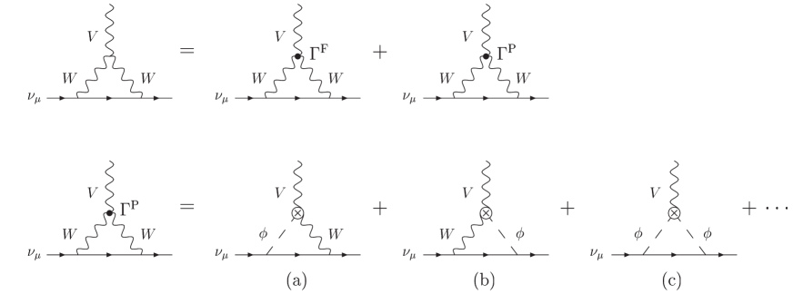
Figure 4: Carrying out the PT procedure for constructing the neutrino charge radius. As a result of the Slavnov-Taylor identities triggered by the longitudinal pinching momenta contained in $\Gamma^{\rm P}$, one obtains the PT terms (a), (b) and (c) that, when added to the corresponding $R_{\xi}$ ones, will project the theory to the Feynman gauge of the background field method. The dots denote propagator like terms.

III Nielsen identities analysis

Recently Binosi:2002ft ; Binosi:2004qe , it has been realized that the fundamental underlying symmetry which is driving the PT cancellations is the Becchi-Rouet-Stora-Tyutin (BRST) symmetry Becchi:1976nq . This realization has been instrumental in generalizing the PT procedure to all orders, and has allowed for its connection to powerful BRST related formalisms. As a result, one can take full advantage of the BRST symmetry to deeper analyze the nature of the PT cancellations discussed in our one-loop example, in general, and the issue of neglecting terms proportional to the masses of the internal fermions, in particular. To this end, we will work within the framework of the Batalin-Vilkovisky Batalin:1977pb and Nielsen Nielsen:1975fs formalisms, which will be briefly reviewed in what follows.

III.1 General formalism

As far as the Batalin-Vilkovisky formalism is concerned, one introduces for each SM field $\Phi$, the corresponding anti-field $\Phi^{*}$, and couples them through the Lagrangian (for details see also Grassi:1999tp ; Binosi:2002ez )

$${\cal L}_{\rm BRST}=\sum_{\Phi}\Phi^{*}s\,\Phi,$$ (30)

where $s$ is the BRST operator. In particular, the coupling of the neutral gauge bosons and scalar BRST sources (denoted by $V^{*}_{\mu}$, and $\chi^{*}$, $H^{*}$ respectively), read

$${\cal L}_{\rm BRST} \supset ig_{\rm w}C_{V}V^{*}_{\mu}(W^{+\mu}c^{-}-W^{-\mu}c^{+})+\frac{g_{\rm w}}{2}\chi^{*}(\phi^{+}c^{-}+\phi^{-}c^{+})-\frac{g_{\rm w}}{2c_{\rm w}}\chi^{*}Hc^{Z}$$ (31)

$$+ \frac{ig_{\rm w}}{2}H^{*}(\phi^{+}c^{-}-\phi^{-}c^{+})+\frac{g_{\rm w}}{2c_{\rm w}}H^{*}\chi c^{Z},$$

$c^{\pm}$ and $c^{V}$ being the charged and neutral ghost fields, respectively. Then from ${\cal L}_{\rm BRST}$, one finds the Feynman rules shown in Fig.5.

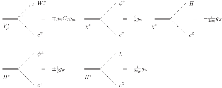
Figure 5: The Feynman rules for the neutral gauge bosons ($V^{*}_{\mu}$) and scalars ($\chi^{*}$, $H^{*}$) BRST sources coming from the Lagrangian ${\cal L}_{\rm BRST}$.

The BRST invariance of the SM action, or, equivalently, the unitarity of the $S$-matrix and the gauge independence of the physical observables, are then encoded into the master equation

$${\mathfrak{S}}(\Gamma)=0,$$ (32)

where

$${\mathfrak{S}}(\Gamma)=\int\!d^{4}x\,\sum_{\Phi}\frac{\delta^{R}\Gamma}{\delta\Phi}\frac{\delta^{L}\Gamma}{\delta\Phi^{*}}.$$ (33)

In Eq.(33), the sum runs over all the SM fields, $R$ and $L$ denote the right and left differentiation, respectively, and $\Gamma$ represents the effective action [which depends on the antifields through Eq.(30)]. This equation can be used to derive the complete set of non-linear STIs to all orders in the perturbative theory, via the repeated application of functional differentiation.

However the important point here is that by enlarging the BRST symmetry of the theory, one can construct a tool that allows to control the dependence of the Green’s functions on the gauge parameter $\xi_{i}$ (with $i={W,V}$) in a completely algebraic way. In fact, let us promote the parameters $\xi_{i}$ to (static) fields, and introduce their corresponding BRST sources $\eta_{i}$, in such a way that

$$s\xi_{i}=\eta_{i},\qquad\qquad s\eta_{i}=0.$$ (34)

After doing this, the BRST invariance of the ghost (${\cal L}_{{\rm FPG}}$) and gauge fixing (${\cal L}_{{\rm GF}}$) sectors of the SM Lagrangian is lost, and to restore it one has to add to the the sum ${\cal L}_{{\rm GF}}+{\cal L}_{{\rm FPG}}$ the term

$${\cal L}_{\rm N}=-\frac{1}{2\xi_{\scriptscriptstyle W}}\eta_{\scriptscriptstyle W}\left(\bar{c}^{+}{\cal F}^{+}+\bar{c}^{-}{\cal F}^{-}\right)-\sum_{V}\frac{1}{2\xi_{V}}\eta_{V}\left(\bar{c}^{V}{\cal F}^{V}\right),$$ (35)

where ${\cal F}^{\pm}$, ${\cal F}^{V}$ represent the gauge fixing functions, i.e.,

$${\cal F}^{\pm}=\partial^{\mu}W^{\pm}_{\mu}\mp i\xi_{W}M_{W}\phi^{\pm},\qquad{\cal F}^{V}=\partial^{\mu}V_{\mu}-\xi_{V}M_{V}\chi,$$ (36)

within the class of $R_{\xi}$ gauges used in our analysis.

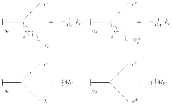
Figure 6: The Feynman rules for the $\eta_{i}$ static sources coming from the Lagrangian ${\cal L}_{\rm N}$.

The term ${\cal L}_{\rm N}$ will then control the couplings of the sources $\eta_{i}$ to the SM fields, giving rise to the Feynman rules shown in Fig.6. For all practical calculations one can set $\eta_{i}=0$ thus recovering both the unextended BRST transformations, as well as the master equation of Eq.(32). However when $\eta_{i}\neq 0$, the master equation reads

$${\mathfrak{S}}_{\eta_{i}}(\Gamma)=0,$$ (37)

where

$${\mathfrak{S}}_{\eta_{i}}(\Gamma)={\mathfrak{S}}(\Gamma)+\eta_{i}\partial_{\xi_{i}}\Gamma.$$ (38)

Thus, after differentiating this new master equation with respect to $\xi_{i}$, and setting $\eta_{i}$ to zero, we obtain

$$\left.\partial_{\xi_{i}}\Gamma\right|_{\eta_{i}=0}=-\left.\left(\int\!d^{4}x\,\partial_{\eta_{i}}\sum_{\Phi}\frac{\delta^{R}\Gamma}{\delta\Phi}\frac{\delta^{L}\Gamma}{\delta\Phi^{*}}\right)\right|_{\eta_{i}=0}.$$ (39)

Establishing the above functional equation, allows, via the repeated application of functional differentiation, to derive a set of identities, known in the literature under the name of NIs Nielsen:1975fs , that control the gauge-parameter(s) dependence of the different Green’s functions appearing in the theory. Therefore, NIs can be used to unveil in their full generality the patterns of gauge cancellations occurring inside gauge independent quantities such as $S$-matrix elements. In fact, as has been demonstrated recently Binosi:2004qe , these patterns are actually of the PT type. Notice, however, that, unlike the PT, NIs cannot be used to construct gauge invariant and gauge-fixing-parameter-independent Green’s functions.

Finally, a technical remark. The extension of the BRST symmetry through Eq.(34) is just a technical trick to gain control over the gauge-parameter dependence of the various Green’s functions appearing in the theory; thus, unlike the STIs generated from Eq.(33), Eq.(39) does not have to be preserved in the renormalization procedure, which will in general deform it (see Gambino:1999ai and references therein). The complications due to this fact may be circumvented by choosing to work within a renormalization scheme that fixes the parameters of ${\cal L}_{\rm SM}^{\rm cl}$ using physical observables (see again Gambino:1999ai ).

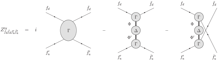
Figure 7: The decomposition of the truncated Green’s function $Z_{f_{d}\bar{f}_{d}f^{\prime}_{u}\bar{f}^{\prime}_{u}}^{\rm tr}$. Notice that the last diagram is not present when $f_{d}$ and $f^{\prime}_{u}$ are not in the same doublet.

Having said that, let $Z_{f_{d}\bar{f}_{d}f^{\prime}_{u}\bar{f}^{\prime}_{u}}^{\rm tr}$ be the truncated Green’s function associated to our four fermion process, where $f_{d}$ (respectively $f^{\prime}_{u}$) represents a down-(respectively, up-) type lepton. If we assume that $f^{\prime}_{u}$ and $f_{d}$ are not in the same doublet, the latter four-point function allows for the following decomposition (see Fig.7)

$$Z_{f_{d}\bar{f}_{d}f^{\prime}_{u}\bar{f}^{\prime}_{u}}^{\rm tr} = i\Gamma_{f_{d}\bar{f}_{d}f^{\prime}_{u}\bar{f}^{\prime}_{u}}-\left(\Gamma_{f_{d}\bar{f}_{d}\Phi}\Delta_{\Phi\Phi^{\prime}}\Gamma_{\Phi^{\prime}f^{\prime}_{u}\bar{f}^{\prime}_{u}}+\Gamma_{f_{d}\bar{f}^{\prime}_{u}\Phi}\Delta_{\Phi\Phi^{\prime}}\Gamma_{\Phi^{\prime}f^{\prime}_{u}\bar{f}_{d}}\right)$$ (40)

$$= i\Gamma_{f_{d}\bar{f}_{d}f^{\prime}_{u}\bar{f}^{\prime}_{u}}-\Gamma_{f_{d}\bar{f}_{d}\Phi}\Delta_{\Phi\Phi^{\prime}}\Gamma_{\Phi^{\prime}f^{\prime}_{u}\bar{f}^{\prime}_{u}},$$

where a sum over repeated fields (running over all the allowed SM combinations) is understood, $\Delta_{\Phi\Phi^{\prime}}(q)$ indicates a (full) propagator between the SM fields $\Phi$ and $\Phi^{\prime}$, and we have omitted the momentum dependence of the Green’s functions as well as Lorentz indices. Then, the gauge invariance of the $S$-matrix implies

$$\partial_{\xi_{i}}Z_{f_{d}\bar{f}_{d}f^{\prime}_{u}\bar{f}^{\prime}_{u}}^{\rm tr} = i\partial_{\xi_{i}}\Gamma_{f_{d}\bar{f}_{d}f^{\prime}_{u}\bar{f}^{\prime}_{u}}$$ (41)

$$- (\partial_{\xi_{i}}\Gamma_{f_{d}\bar{f}_{d}\Phi})\Delta_{\Phi\Phi^{\prime}}\Gamma_{\Phi^{\prime}f^{\prime}_{u}\bar{f}^{\prime}_{u}}-\Gamma_{f_{d}\bar{f}^{\prime}_{d}\Phi}(\partial_{\xi_{i}}\Delta_{\Phi\Phi^{\prime}})\Gamma_{\Phi^{\prime}f^{\prime}_{u}\bar{f}^{\prime}_{u}}-\Gamma_{f_{d}\bar{f}_{d}\Phi}\Delta_{\Phi\Phi^{\prime}}(\partial_{\xi_{i}}\Gamma_{\Phi^{\prime}f^{\prime}_{u}\bar{f}^{\prime}_{u}})$$

$$= 0.$$

The NIs can be used to determine how the perturbative series rearranges itself in order to fulfill the above equality. Neglecting terms that either vanish due to the on-shell conditions of the external fermions or cancel when using the LSZ reduction formula, the NIs for the various terms that appear in Eq.(41) can be derived from the master equation (39), and read

$$\partial_{\xi_{i}}\Delta_{\Phi\Phi^{\prime}} = \Delta_{\Phi\Phi^{\prime\prime}}\Gamma_{\eta_{i}\Phi^{\prime\prime}{\Phi^{\prime}}^{*}}+\Gamma_{\eta_{i}\Phi^{*}\Phi^{\prime\prime}}\Delta_{\Phi^{\prime\prime}\Phi^{\prime}},$$

$$-\partial_{\xi_{i}}\Gamma_{f\bar{f}\Phi} = \Gamma_{\eta_{i}{\Phi^{\prime}}^{*}f\bar{f}}\Gamma_{\Phi^{\prime}\Phi}+\Gamma_{\eta_{i}\Phi{\Phi^{\prime}}^{*}}\Gamma_{\Phi^{\prime}f\bar{f}},$$

$$-\partial_{\xi_{i}}\Gamma_{f_{d}\bar{f}_{d}f^{\prime}_{u}\bar{f}^{\prime}_{u}} = \Gamma_{f_{d}\bar{f}_{d}\Phi}\Gamma_{\eta_{i}{\Phi}^{*}f^{\prime}_{u}\bar{f}^{\prime}_{u}}+\Gamma_{f_{d}\bar{f}^{\prime}_{u}\Phi}\Gamma_{\eta_{i}{\Phi}^{*}f^{\prime}_{u}\bar{f}_{d}}+\Gamma_{\eta_{i}{\Phi}^{*}f_{d}\bar{f}_{d}}\Gamma_{\Phi f^{\prime}_{u}\bar{f}^{\prime}_{u}}+\Gamma_{\eta_{i}{\Phi}^{*}f_{d}\bar{f}^{\prime}_{u}}\Gamma_{\Phi f^{\prime}_{u}\bar{f}_{d}}$$ (42)

$$= \Gamma_{f_{d}\bar{f}_{d}\Phi}\Gamma_{\eta_{i}{\Phi}^{*}f^{\prime}_{u}\bar{f}^{\prime}_{u}}+\Gamma_{\eta_{i}{\Phi}^{*}f_{d}\bar{f}_{d}}\Gamma_{\Phi f^{\prime}_{u}\bar{f}^{\prime}_{u}}.$$

Notice that despite their appearance, the four point functions $\Gamma_{\eta_{i}{\Phi}^{*}f\bar{f}}$ (respectively, the three point functions $\Gamma_{\eta_{i}\Phi{\Phi^{\prime}}^{*}}$) are vertex-like (respectively propagator-like), due to the static nature of the $\eta_{i}$ sources.

As far as the cancellations of gauge-dependent pieces are concerned, we see that the gauge-fixing-parameter-dependence of the internal self-energies cancels according to the pattern

$$\Gamma_{f_{d}\bar{f}_{d}\Phi}(\Delta_{\Phi\Phi^{\prime\prime}}\Gamma_{\eta_{i}\Phi^{\prime\prime}{\Phi^{\prime}}^{*}}+\Gamma_{\eta_{i}\Phi^{*}\Phi^{\prime\prime}}\Delta_{\Phi^{\prime\prime}\Phi^{\prime}})\Gamma_{\Phi^{\prime}f^{\prime}_{u}\bar{f}^{\prime}_{u}}$$ (43)

$$- (\Gamma_{\eta_{i}\Phi{\Phi^{\prime\prime}}^{*}}\Gamma_{\Phi^{\prime\prime}f_{d}\bar{f}^{\prime}_{d}})\Delta_{\Phi\Phi^{\prime}}\Gamma_{\Phi^{\prime}f^{\prime}_{u}\bar{f}^{\prime}_{u}}+\Gamma_{f_{d}\bar{f}_{d}\Phi}\Delta_{\Phi\Phi^{\prime}}(\Gamma_{\eta_{i}\Phi^{\prime}{\Phi^{\prime\prime}}^{*}}\Gamma_{\Phi^{\prime\prime}f_{d}\bar{f}_{d}})=0.$$

Using finally, the relation $\Delta_{\Phi\Phi^{\prime\prime}}\Gamma_{\Phi^{\prime\prime}\Phi^{\prime}}=i\delta_{\Phi\Phi^{\prime}}$, one can uncover the cancellation happening between the boxes and vertices, according to the rules

$$-i\Gamma_{\Phi f_{d}\bar{f}_{d}}\Gamma_{\eta_{i}{\Phi}^{*}f_{u}\bar{f}_{u}}+\Gamma_{f_{d}\bar{f}_{d}\Phi}\Delta_{\Phi\Phi^{\prime}}\Gamma_{\Phi^{\prime}\Phi^{\prime\prime}}\Gamma_{\eta_{i}{\Phi^{\prime\prime}}^{*}f^{\prime}_{u}\bar{f}^{\prime}_{u}} = 0$$

$$-i\Gamma_{\eta_{i}{\Phi}^{*}f_{d}\bar{f}_{d}}\Gamma_{f^{\prime}_{u}\bar{f}^{\prime}_{u}\Phi}+\Gamma_{\eta_{i}{\Phi^{\prime\prime}}^{*}f_{d}\bar{f}_{d}}\Gamma_{\Phi^{\prime\prime}\Phi}\Delta_{\Phi\Phi^{\prime}}\Gamma_{\Phi^{\prime}f^{\prime}_{u}\bar{f}^{\prime}_{u}} = 0.$$ (44)

From the above patterns one concludes that the gauge cancellations: (i) go through without the need of integration over the virtual momenta; (ii) follow the $s$-$t$ cancellations characteristic of the PT (which, in a sense, is to be expected since both the PT cancellations and the NIs are BRST-driven); (iii) proceed regardless of whether the fermions are massive or massless.

III.2 The one-loop case re-examined

In order to make the conclusions drawn at the end of the previous section more quantitative, we consider the one-loop case already addressed in the PT framework, and identify the pieces that cancel between box and vertex diagrams in the NIs. At one-loop level, the third equation in (42), reads

$$-\partial_{\xi_{i}}\Gamma^{(1)}_{f_{d}\bar{f}_{d}f^{\prime}_{u}\bar{f}^{\prime}_{u}}=\Gamma^{(0)}_{f_{d}\bar{f}_{d}\Phi}\Gamma^{(1)}_{\eta_{i}{\Phi}^{*}f^{\prime}_{u}\bar{f}^{\prime}_{u}}+\Gamma^{(1)}_{\eta_{i}{\Phi}^{*}f_{d}\bar{f}_{d}}\Gamma^{(0)}_{\Phi f^{\prime}_{u}\bar{f}^{\prime}_{u}}.$$ (45)

We are interested in the case where $\xi_{i}=\xi_{\scriptscriptstyle W}$ (it is immediate to show from the above equation and the Feynman rules provided in Fig.5 and 6, that boxes involving neutral gauge bosons form a gauge independent sub-set, at this order), so that one has

$$-\partial_{\xi_{\scriptscriptstyle W}}\Gamma^{(1)}_{f_{d}\bar{f}_{d}f^{\prime}_{u}\bar{f}^{\prime}_{u}} = \Gamma^{(0)}_{f_{d}\bar{f}_{d}\Phi}\Gamma^{(1)}_{\eta_{\scriptscriptstyle W}{\Phi}^{*}f^{\prime}_{u}\bar{f}^{\prime}_{u}}+\Gamma^{(1)}_{\eta_{\scriptscriptstyle W}{\Phi}^{*}f_{d}\bar{f}_{d}}\Gamma^{(0)}_{\Phi f^{\prime}_{u}\bar{f}^{\prime}_{u}}$$ (46)

$$= \Gamma^{(0)}_{f_{d}\bar{f}_{d}V^{\mu}}\Gamma^{(1)}_{\eta_{\scriptscriptstyle W}V^{*}_{\mu}f^{\prime}_{u}\bar{f}^{\prime}_{u}}+\Gamma^{(1)}_{\eta_{\scriptscriptstyle W}V^{*}_{\mu}f_{d}\bar{f}_{d}}\Gamma^{(0)}_{V^{\mu}f^{\prime}_{u}\bar{f}^{\prime}_{u}}+\Gamma^{(0)}_{f_{d}\bar{f}_{d}S}\Gamma^{(1)}_{\eta_{\scriptscriptstyle W}S^{*}f^{\prime}_{u}\bar{f}^{\prime}_{u}}.$$

Introducing the kernels ${\cal K}$ according to Fig.8, one has

$$\Gamma^{(0)}_{f_{d}\bar{f}_{d}V^{\mu}}\Gamma^{(1)}_{\eta_{\scriptscriptstyle W}V^{*}_{\mu}f^{\prime}_{u}\bar{f}^{\prime}_{u}} = -g_{\rm w}C_{V}\Gamma^{(0)}_{V^{\mu}f_{d}\bar{f}_{d}}\bigg{[}{\cal K}^{W,(1)}_{u\,\mu}+{\cal K}^{\phi,(1)}_{u\,\mu}\bigg{]},$$

$$\Gamma^{(1)}_{\eta_{\scriptscriptstyle W}V^{*}_{\mu}f_{d}\bar{f}_{d}}\Gamma^{(0)}_{V^{\mu}f^{\prime}_{u}\bar{f}^{\prime}_{u}} = -g_{\rm w}\left[{\cal K}^{W,(1)}_{d\,\mu}+{\cal K}^{\phi,(1)}_{d\,\mu}\right]C_{V}\Gamma^{(0)}_{V^{\mu}f^{\prime}_{u}\bar{f}^{\prime}_{u}},$$

$$\Gamma^{(0)}_{f_{d}\bar{f}_{d}S}\Gamma^{(1)}_{\eta_{\scriptscriptstyle W}S^{*}f^{\prime}_{u}\bar{f}^{\prime}_{u}} = -g_{\rm w}\left[{\cal K}^{W,(1)}_{d}+{\cal K}^{\phi,(1)}_{d}\right]\left(ig_{\rm w}\frac{m_{f_{d}}}{M_{W}}P_{L}\right).$$ (47)

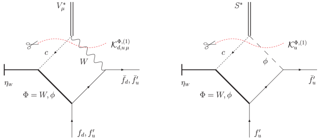
Figure 8: The (one particle irreducible) diagrams contributing to the NI of the one loop box diagrams of the $f_{d}f^{\prime}_{u}\to f_{d}f^{\prime}_{u}$ process. Notice that since the sources $\eta_{i}$ are static, these diagrams are vertex-like. The associated kernels ${\cal K}$ is also shown, and is obtained by simply factoring out from the corresponding diagram the vertex involving the antifield.

Now, consider first of all the case in which the down-type target fermion $f_{d}$ is massless and right-handedly polarized (i.e., a pure positive helicity state), as was done in Bernabeu:2000hf . Then we know that the contribution from the box diagram with two $W$s is zero (there is no $\Gamma^{(0)}_{W_{\mu}f^{R}_{d}\bar{f}^{R}_{d}}$ vertex in this case); thus, the left-hand side of Eq.(46) vanishes identically. As far as the right-hand side is concerned, the third term vanishes because $m_{f_{d}}=0$, the second term because the corresponding kernels in Eq.(47) are zero, while the first one due to the relation (making explicit the sum over the neutral gauge bosons)

$$\sum_{V}C_{V}\Gamma^{(0)}_{f^{R}_{d}\bar{f}^{R}_{d}V^{\mu}}=0,$$ (48)

which is precisely the current relation employed by the PT Bernabeu:2000hf . Of course, due to Eq.(44) this will be the cancellation pattern followed by the vertex-like gauge-dependent part of the $\Gamma^{(1)}_{A_{\mu}f^{\prime}_{u}\bar{f}^{\prime}_{u}}$ and $\Gamma^{(1)}_{Z_{\mu}f^{\prime}_{u}\bar{f}^{\prime}_{u}}$ vertices.

Next, one can consider the case in which the target fermions $f_{d}$ are massless, but unpolarized. Then, while the third term of Eq.(47) continue to be zero, the second one is not, and it is needed to cancel the vertex-like gauge dependence of the vertex $\Gamma^{(1)}_{Z_{\mu}f_{d}\bar{f}_{d}}$ which is now present. The first term, which cancels the vertex-like gauge-dependent part of the $\Gamma^{(1)}_{A_{\mu}f^{\prime}_{u}\bar{f}^{\prime}_{u}}$ and $\Gamma^{(1)}_{Z_{\mu}f^{\prime}_{u}\bar{f}^{\prime}_{u}}$ vertices, is now proportional to

$$-\sum_{V}C_{V}\Gamma^{(0)}_{f_{d}\bar{f}_{d}V^{\mu}}=-i\frac{g_{\rm w}}{2}\gamma_{\mu}P_{\!\scriptscriptstyle{L}},$$ (49)

which is precisely the current relation (with the spinors suppressed) of Eq.(26). Notice that the NIs show immediately that the above PT gauge cancellation pattern is the same regardless of whether the iso-doublet partner of the $f^{\prime}_{u}$ fermions are massless (as in Bernabeu:2000hf ) or massive (as in Section II.3).

Finally, we see that relaxing the hypothesis of massless down-type target fermions does not distort the cancellations described in the previous case: the only difference is that the third term is no longer zero, since it is needed to cancel the gauge dependent part coming from the $\Gamma^{(1)}_{Sf^{\prime}_{u}\bar{f}^{\prime}_{u}}$ which is now present.

Thus we see that considering the down-type fermion to be massless or massive, has no bearing whatsoever on one’s ability to implement the gauge cancellations following the PT algorithm.

III.3 All-order considerations

We next show that the pattern of gauge-cancellations which has been unravelled at one-loop level persists to all orders in perturbation theory. In particular, we will show that at higher orders the gauge-dependent terms stemming from the conventional vertex (which would naively form part of the NCR definition) cancel against similar vertex-like terms coming from box diagrams, folowing a pattern identical to that operating at one-loop. Thus, these gauge-dependent terms drop out from the NCR definition in a natural way, at any order in the perturbative expansion,

The term we need to study is the vertex-like contribution coming from the $\Gamma_{f_{d}\bar{f}_{d}V_{\mu}}\Delta_{V^{\mu}\Phi}(\partial_{\xi_{\scriptscriptstyle W}}\Gamma_{\Phi f^{\prime}_{u}\bar{f}^{\prime}_{u}})$ piece of Eq.(41). After employing the second of Eqs.(42), we get (discarding the propagator-like part)

$$-\Gamma_{f_{d}\bar{f}_{d}V_{\mu}}\Delta_{V^{\mu}\Phi}(\partial_{\xi_{\scriptscriptstyle W}}\Gamma_{\Phi f^{\prime}_{u}\bar{f}^{\prime}_{u}}) = \Gamma_{f_{d}\bar{f}_{d}V_{\mu}}\Delta_{V^{\mu}\Phi}\Gamma_{\Phi\Phi^{\prime}}\Gamma_{\eta_{i}{\Phi^{\prime}}^{*}f^{\prime}_{u}\bar{f}^{\prime}_{u}}$$ (50)

$$= i\Gamma_{f_{d}\bar{f}_{d}V_{\mu}}\Gamma_{\eta_{\scriptscriptstyle W}V^{\mu*}f^{\prime}_{u}\bar{f}^{\prime}_{u}}.$$

Now, from the Feynman rules of Fig.5, one has that the vertex involving the neutral gauge bosons anti-field $A^{*}_{\mu}$ is connected to the one involving the $Z^{*}_{\mu}$ anti-field through the relation

$$c_{\rm w}\Gamma_{A^{*}_{\mu}W^{\pm}_{\nu}c^{\mp}}=-s_{\rm w}\Gamma_{Z^{*}_{\mu}W^{\pm}_{\nu}c^{\mp}}.$$ (51)

On the other hand, since the $\eta_{\scriptscriptstyle W}$ source couples to charged fields only (see Fig.6), the three-point functions $\Gamma_{\eta_{\scriptscriptstyle W}V^{*}_{\mu}f\bar{f}}$ appearing in the NIs will be such that

$$c_{\rm w}\Gamma_{\eta_{\scriptscriptstyle W}A^{*}_{\mu}f\bar{f}}=-s_{\rm w}\Gamma_{\eta_{\scriptscriptstyle W}Z^{*}_{\mu}f\bar{f}}.$$ (52)

Therefore, introducing the kernels ${\cal K}^{\Phi}_{u}$ as the dressed version of the ones employed in the one-loop analysis of the previous section (see also Fig.8), this last equation shows that the NCR gauge-dependent terms of Eq.(50) are of the form (making explicitly the sum over the neutral gauge bosons)

$$i\sum_{V}C_{V}\Gamma_{f_{d}\bar{f}_{d}V^{\mu}}{\cal K}^{\Phi}_{\mu},$$ (53)

which is nothing but a direct higher order version of the identity of Eq.(49), encountered in the one-loop analysis. This term will be precisely cancelled by the box contribution $-i\Gamma_{f_{d}\bar{f}_{d}V^{\mu}}\Gamma_{\eta_{\scriptscriptstyle W}V^{\mu*}f^{\prime}_{u}\bar{f}^{\prime}_{u}}$ appearing in the first formula of Eq.(44).

IV Conclusions

In this article we have addressed theoretical issues related to the proper definition of the gauge-independent SM vertex describing the effective interaction between a neutrino and an off-shell photon, together with the electromagnetic form factor and the corresponding NCR obtained by it. This effective vertex has been constructed at one-loop in Bernabeu:2000hf , in the framework of the PT, under the operational assumption that the mass of the iso-doublet partner of the neutrino under consideration was vanishing (except in infra-red divergent expressions). In the first part of the present article we have demonstrated through an explicit calculation that any additional gauge-dependent contributions proportional to the fermion masses cancel partially against similar contributions stemming from graphs containing would-be Goldstone bosons, and partially against vertex-like contributions concealed inside box-graphs. This cancellation proceeds precisely as the well-defined PT methodology dictates, without any additional assumptions This completes the proof that the properties of the effective NCR listed in the Introduction maintain their validity in the presence of massive fermions. In the second part of the paper we have employed the powerful formalism of the Nielsen identities, and furnished an all-order demonstration of the relevant gauge-cancellations, a fact which finally allows for the all-order definition of the effective NCR.

Acknowledgments: This work has been supported by the CICYT Grant FPA2002-00612.

References

- (1) J. Bernstein and T. D. Lee, Phys. Rev. Lett. 11, 512 (1963); W. A. Bardeen, R. Gastmans and B. Lautrup, Nucl. Phys. B 46 (1972) 319; S. Y. Lee, Phys. Rev. D 6, 1701 (1972); A. D. Dolgov and Y. B. Zeldovich, Rev. Mod. Phys. 53, 1 (1981).
- (2) Of course, the covariant generalization of this definition, just as that of a static charge distribution, is ambiguous.
- (3) J. L. Lucio, A. Rosado and A. Zepeda, Phys. Rev. D 29, 1539 (1984); N. M. Monyonko and J. H. Reid, Prog. Theor. Phys. 73, 734 (1985); A. Grau and J. A. Grifols, Phys. Lett. B 166, 233 (1986); G. Auriemma, Y. Srivastava and A. Widom, Phys. Lett. 195B, 254 (1987) [Erratum-ibid. 207B, 519 (1988)]; P. Vogel and J. Engel, Phys. Rev. D 39, 3378 (1989); G. Degrassi, A. Sirlin and W. J. Marciano, Phys. Rev. D 39, 287 (1989); M. J. Musolf and B. R. Holstein, Phys. Rev. D 43, 2956 (1991); K. L. Ng, Z. Phys. C 55, 145 (1992); L. G. Cabral-Rosetti, J. Bernabeu, J. Vidal and A. Zepeda, Eur. Phys. J. C 12, 633 (2000).
- (4) J. M. Cornwall, Phys. Rev. D 26, 1453 (1982); J. M. Cornwall and J. Papavassiliou, Phys. Rev. D 40, 3474 (1989); J. Papavassiliou, Phys. Rev. D 41, 3179 (1990).
- (5) J. Bernabeu, L. G. Cabral-Rosetti, J. Papavassiliou and J. Vidal, Phys. Rev. D 62, 113012 (2000).
- (6) J. Bernabeu, J. Papavassiliou and J. Vidal, Phys. Rev. Lett. 89, 101802 (2002) [Erratum-ibid. 89, 229902 (2002)]
- (7) J. Bernabeu, J. Papavassiliou and J. Vidal, Nucl. Phys. B 680, 450 (2004)
- (8) J. Papavassiliou, J. Bernabeu, D. Binosi and J. Vidal, arXiv:hep-ph/0310028.
- (9) K. Fujikawa and R. Shrock, Phys. Rev. D 69, 013007 (2004)
- (10) N. K. Nielsen, Nucl. Phys. B 101, 173 (1975).
- (11) J. M. Cornwall and G. Tiktopoulos, Phys. Rev. D 15, 2937 (1977).
- (12) G. Degrassi and A. Sirlin, Phys. Rev. D 46, 3104 (1992).
- (13) K. Hagiwara, S. Matsumoto, D. Haidt and C. S. Kim, Z. Phys. C 64, 559 (1994) [Erratum-ibid. C 68, 352 (1994)]; J. Papavassiliou, E. de Rafael and N. J. Watson, Nucl. Phys. B 503, 79 (1997); J. Papavassiliou and A. Pilaftsis, Phys. Rev. D 58, 053002 (1998)
- (14) P. Salati, Astropart. Phys. 2, 269 (1994); R. C. Allen et al., Phys. Rev. D 43, 1 (1991); A. M. Mourao, J. Pulido and J. P. Ralston, Phys. Lett. B 285, 364 (1992) [Erratum-ibid. B 288, 421 (1992)]; P. Vilain et al. [CHARM-II Collaboration], Phys. Lett. B 345, 115 (1995); J. A. Grifols and E. Masso, Mod. Phys. Lett. A 2, 205 (1987); J. A. Grifols and E. Masso, Phys. Rev. D 40, 3819 (1989); A. S. Joshipura and S. Mohanty, arXiv:hep-ph/0108018; M. Hirsch, E. Nardi and D. Restrepo, Phys. Rev. D 67, 033005 (2003).
- (15) D. Binosi and J. Papavassiliou, Phys. Rev. D 66, 111901 (2002); J. Phys. G 30, 203 (2004).
- (16) D. Binosi, arXiv:hep-ph/0401182; J. Phys. G to appear.
- (17) C. Becchi, A. Rouet and R. Stora, Annals Phys. 98, 287 (1976); I. V. Tyutin, LEBEDEV-75-39.
- (18) I. A. Batalin, G. A. Vilkovisky, Phys. Lett. B69, 309 (1977); Phys. Rev. D28, 2567 (1983).
- (19) P. A. Grassi, T. Hurth, M. Steinhauser, Annals Phys. 288, 197 (2001); Nucl. Phys. B 610, 215 (2001).
- (20) D. Binosi, J. Papavassiliou, Phys. Rev. D 66, 025024 (2002).
- (21) P. Gambino, P. A. Grassi, Phys. Rev. D 62, 076002 (2000).