Unquenching the Quark-Antiquark Green’s Function

Abstract

We propose a nonperturbative resummation scheme for the four-point connected quark-antiquark Green’s function $G^{4}$ that shows how the Bethe–Salpeter equation may be ‘unquenched’ with respect to quark-antiquark loops. This mechanism allows to dynamically account for hadronic meson decays and multiquark structures whilst respecting the underlying symmetries. An initial approximation to the four-point Schwinger–Dyson equation – suitable for phenomenological application – is examined numerically in a couple of aspects. It is demonstrated that this approximation explicitly maintains the correct asymptotic limits and contains the physical resonance structures in the near timelike region in the quark-antiquark channel whereas no resonances are found in the diquark channel, respectively.

I Introduction

For many years, quantum chromo-dynamics (QCD) has been widely accepted as the underlying theory of the strong interaction. As an $SU(N_{c})$ gauge-field theory, QCD has as its elementary particle degrees of freedom the quarks and gluons, whereas the observables of the strong interaction are the spectra of hadrons and their spectral properties. One of the contemporary goals of QCD is clearly a detailed understanding of how the quark and gluon fields give rise to the formations of hadrons within a single theoretical framework. Whereas lattice calculations of QCD have shown substantial progress in the last years of dealing with dynamical fermions and improved actions lattice1 , final and robust results for light quark masses in the continuum limit are still lacking nowadays.

In the absence of a final and complete solution to QCD one is motivated to adopt more pragmatic approaches to gain further insight to the strong interaction and its bound states. The Schwinger–Dyson equations are the field theoretical equivalent of the equations of motion for the theory (see maris03 ; roberts00 ; alkofer00 ; roberts94 for recent reviews); they are dynamical equations in the continuum and embody all those symmetries that define the initial theory such as symmetry under Poincaré transforms, the gauge symmetry, the discrete parity and charge conjugation symmetries and the (broken) chiral symmetry. The inclusion of all of these vital physical features gives an impetus to their study. However, the Schwinger–Dyson equations form an infinite hierarchy of coupled equations that must be truncated to some degree if actual numerical solutions are addressed. Contemporary truncation schemes have two guiding principles: i) the explicit maintaining of as many of the underlying symmetries as feasible and ii) agreement of the final results with observation (and possibly other approaches).

The Schwinger–Dyson equations are coupled non-linear integral equations relating the Green’s functions (as ‘building blocks’) of the theory to one another. By themselves these Green’s functions do not have a physical interpretation but must be combined in various ways to construct physically observable quantities. One particularly efficacious framework munczek83 ; jain93 ; burden96 is the Schwinger–Dyson equation for the quark propagator (gap equation) within the rainbow truncation as input into the ladder Bethe–Salpeter equation. The latter is itself a special case of a Schwinger–Dyson equation which leads to a description of the pion as an (almost massless) Goldstone boson – associated with chiral symmetry breaking – as well as a bound state of two (massive) constituent quarks. The mass of the constituent quarks here is dynamically generated from the spontaneously broken chiral symmetry. The success of this construction in simultaneously describing two of the most fundamental aspects of hadron phenomenology can be traced back to the fact that the truncations employed explicitly observe the relationship imposed by the (flavor non-singlet) axialvector Ward-Takahashi identity (AXWTI) maris97b ; delbourgo79 . The AXWTI is an expression for gauge invariance when applied to quark-axialvector vector Green’s functions. This shows the supreme role of symmetries when applied to dynamical systems. The light pseudoscalar and vector meson masses and leptonic decay constants maris99a ; me02 as well as electromagnetic form factors maris02 ; maris99b are well reproduced with few parameters. In principle such parameters may be fixed by comparison with related quantities from lattice-QCD bhagwat03 .

Whilst the success of the coupled rainbow-ladder Schwinger–Dyson – Bethe–Salpeter framework is laudable, it has so far proved difficult to go beyond this initial (simplest) truncation scheme. There have been several attempts to address different aspects of possible extensions. For example by using effective interactions characterized by $\delta-$functions to resumm classes of diagrams bender96 ; detmold02 and employing hybrid combinations of finite width and $\delta-$function interactions ongoing04 . Ironically, it is the AXWTI that – preserving the symmetry – leads to a rapid increase of effort as one increases the level of sophistication in the truncation scheme.

There are several issues of hadronic physics that the coupled Schwinger–Dyson – Bethe–Salpeter framework has not addressed so far. The first of these is the hadronic decay of mesons, e.g. the decay $\rho\rightarrow\pi\pi$. This question has been investigated within the impulse approximation and acceptable results have been obtained for the decays of vector mesons jarecke02 ; however, the desired genuinely dynamic description is lacking. A second issue is the light scalar spectrum (cf. ref. pennington03 for an introduction to this topic). It is not clear presently, whether the lightest scalar mesons are simple quark-antiquark resonances or if they are dominated by meson-meson, perhaps even diquark-diquark correlations. These issues are connected to unquenching, i.e. the inclusion of internal quark-loops to Bethe–Salpeter amplitudes. The inclusion of such loops allows for multiple quark-antiquark or quark-quark correlations within the overall Bethe–Salpeter amplitude; these correlations give rise to the decay mechanisms and internal multiquark structures. Clearly then, such internal correlations play a significant role in the dynamical description of hadrons. The four-point connected quark-antiquark Green’s function ($G^{4}$) is the simplest (and key quantity) of such correlations.

The aim of this paper is: i) to motivate the study of the 4-pt quark-antiquark Green’s function with a practical example for future more extended studies, ii) to show how a phenomenologically useful, dynamically generated approximation can be constructed, and iii) to show actual numerical results. The example chosen is the unquenching of the Bethe–Salpeter kernel in a manner that preserves the AXWTI, maintains the charge conjugation properties and allows for the dynamical description of meson decay widths and possible multiquark systems.

Throughout this paper we work in the isospin ($d=u$) limit with the only distinction between quark flavors being their current mass. We take two light flavors of quark, up and strange, and consider only the flavor non-singlet eigenstates $\overline{u}u$, $\overline{s}u$ and $\overline{s}s$. This means that we do not consider the effects of (isosinglet and singlet) flavor mixing, such as the $U(1)_{A}$ anomaly induced in the $\eta-\eta^{\prime}$ system, but rather focus on pure flavor eigenstates. We work in Euclidean space throughout, metric $\delta_{\mu\nu}$ and with Hermitian Dirac matrices that obey $\{\gamma_{\mu},\gamma_{\nu}\}=2\delta_{\mu\nu}$. The integral measure is $\,\,\,\raisebox{-1.72218pt}{\large$\bar{}$}\!\!d\,{k}\,=d^{4}k/(2\pi)^{4}$.

II Unquenching the Bethe–Salpeter Kernel

The ‘unquenching’ of a system entails allowing insertion of arbitrary numbers of internal quark loops into the various amplitudes of the system. Fully unquenching the system is clearly tantamount to solving a major component of the theory, which of course is beyond present techniques. However, as a first step we consider a restricted class of unquenching terms that include only a single quark loop and are diagrammatically planar. Hereafter, we refer to unquenching as the insertion of this single quark loop.

As a prelude to unquenching the system we consider the fully amputated, connected quark-antiquark (4-pt) Green’s function $G^{4}$ that is two-particle irreducible with respect to any quark-antiquark pair under the ladder truncation. It obeys the Schwinger–Dyson equation (shown graphically in Fig. 1)

$$G_{\alpha\beta;\delta\gamma}^{4}(p_{+},p_{-};k_{-},k_{+})=D_{\mu\nu}^{ab}(p_{+}-k_{+})[V_{\mu}^{a}]_{\alpha\gamma}[V_{\nu}^{b}]_{\delta\beta}$$ (1)

$$+\int\,\,\,\raisebox{-1.72218pt}{\large$\bar{}$}\!\!d\,{q}\,G_{\alpha\beta;\tau\kappa}^{4}(p_{+},p_{-};q_{-},q_{+})[S_{1}(q_{+})V_{\mu}^{a}]_{\kappa\gamma}[V_{\nu}^{b}S_{2}(q_{-})]_{\delta\tau}\overline{D}_{\mu\nu}^{ab}(q_{+}-k_{+}).$$

Figure 1: Schwinger–Dyson equation for the fully amputated, connected quark-antiquark (4-pt) Green’s function, two-particle irreducible with respect to quark-antiquark pairs under the ladder truncation. Internal propagators here are fully dressed.

In the above equation

$$S_{i}(p)=-\imath\hbox to0.0pt{\hbox to5.03125pt{\hfil/\hfil}\hss}pv_{i}(p^{2})+s_{i}(p^{2})$$ (2)

denotes the quark propagator of flavor $i$ and

$$V_{\mu}^{a}=\imath T^{a}\gamma_{\mu}$$ (3)

is the tree-level quark-gluon vertex. $D_{\mu\nu}^{ab}(q)$ and $\overline{D}_{\mu\nu}^{ab}(q)$ are two different effective interaction terms, one for the seed term and one for the kernel of the equation. The reader might be worried about two different interactions terms, however, the reason for this separation will become clear in later sections and allow for practical truncation schemes that obey the underlying symmetries. Note, furthermore, that the distinction of seed and kernel interactions leads to an asymmetry between left and right quark-antiquark pairs. The momenta are given by $p_{\pm}=p\pm Q/2$, similarly for $k$ and $q$.

Equation (1) – under the assumption that the $G^{4}$ contains resonant components in the timelike $s$-channel – can be used as a starting point for the derivation of the ladder truncation of the Bethe–Salpeter equation (see for example nakanishi69 ). As mentioned in the introduction earlier, these resonant components well describe the light pseudoscalar and vector mesons (the latter albeit in the case where meson decay is neglected). We emphasize though that Eq. (1), unlike the Bethe–Salpeter equation, contains both the resonant and non-resonant components in a single expression.

With the above 4-pt function ($G^{4}$) in mind we propose the truncated quark Schwinger–Dyson equation

$$S^{-1}_{\alpha\rho}(p)=\imath\hbox to0.0pt{\hbox to5.03125pt{\hfil/\hfil}\hss}p+m-\int\,\,\,\raisebox{-1.72218pt}{\large$\bar{}$}\!\!d\,{k}\,[V_{\mu}^{a}S(k)V_{\nu}^{b}]_{\alpha\rho}D_{\mu\nu}^{ab}(p-k)$$

$$+\int\,\,\,\raisebox{-1.72218pt}{\large$\bar{}$}\!\!d\,{k}\,\,\,\,\raisebox{-1.72218pt}{\large$\bar{}$}\!\!d\,{q}\,G_{\alpha\beta,\delta\gamma}^{4}(p,p+q;k+q,k)[S(p+q)V_{\mu}^{a}S(k+q)]_{\beta\delta}[S(k)V_{\nu}^{b}]_{\gamma\rho}D_{\mu\nu}^{ab}(p-k).$$

This equation is shown diagrammatically in Fig. 2. The first term of the self-energy is the standard rainbow truncation. The next term gives rise to unquenching since the 4-pt function $G^{4}$ (top line of Fig. 2), when expanded (lower lines), generates planar graphs involving a single internal quark loop connected to the original quark line by successive numbers of gluon exchanges. By identification of the internal ladder graphs we collect those terms whose sum has been shown to give rise to physical resonances (at timelike momenta). The exterior interaction factors are given by $D$, whereas the purely interior interactions are provided by $\overline{D}$; this will preserve the charge conjugation properties of the quark propagator (the left-right asymmetry of $G^{4}$ has been chosen accordingly). In the unexpanded form of the unquenching term, the explicit occurrence of the interaction $D$ and the tree-level quark-gluon vertex $V_{\nu}^{b}$ is to maintain the proper counting of the various graphs in the expansion. The explicit factoring of one tree-level vertex in each dressing term is a general feature of Schwinger–Dyson equations and is maintained here. Equations (LABEL:eq:qdse2) and (1), once $D$ and $\overline{D}$ have been specified, form a closed system which can be solved numerically and naturally includes possible resonance structures in the integrand at timelike momenta. One can regard the multiple gluon exchange terms in the unquenched quark Schwinger–Dyson equation as either a correction to the gluon propagator and/or vertex function or as a nonperturbative dressing of the quark by higher order correlations.

Figure 2: Proposed truncation of the quark Schwinger–Dyson equation to include a single quark loop with the use of the 4-pt function $G^{4}$. All internal propagators are dressed. Springs represent the effective interaction $D$ whereas wavy lines represent the interaction $\overline{D}$ (see text).

The homogeneous quark-antiquark Bethe–Salpeter equation is

$$\Gamma_{\alpha\beta}(p;P)=\int\,\,\,\raisebox{-1.72218pt}{\large$\bar{}$}\!\!d\,{k}\,K_{\alpha\beta;\delta\gamma}(p,k;P)\left[S_{1}(k_{+})\Gamma(k;P)S_{2}(k_{-})\right]_{\gamma\delta}$$ (5)

and the pole condition $P^{2}=-M^{2}$ can be found once the kernel $K$ and the quark propagators $S_{i}$ are specified. As emphasized earlier, the pion can be interpreted as the Goldstone boson of chiral symmetry breaking maris97b when the kernel and the quark self-energy are related such that the AXWTI is satisfied. The flavor non-singlet AXWTI can be expressed in the following way ongoing04

$$[S^{-1}(p_{+})\gamma_{5}+\gamma_{5}S^{-1}(p_{-})]_{\alpha\beta}=[-\imath\gamma_{5}\hbox to0.0pt{\hbox to7.80904pt{\hfil/\hfil}\hss}P+2m\gamma_{5}]_{\alpha\beta}+\int\,\,\,\raisebox{-1.72218pt}{\large$\bar{}$}\!\!d\,{k}\,K(p,k;P)_{\alpha\beta,\delta\gamma}[\gamma_{5}S(k_{-})+S(k_{+})\gamma_{5}]_{\gamma\delta}.$$ (6)

There are two facets to this relation: on one hand, as a Ward-Takahashi type identity it is the expression of the underlying gauge symmetry written in a particular channel and is genuinely nonperturbative in nature; on the other hand it can be expanded semi-perturbatively to reveal relationships between different types of graphs. The former interpretation is responsible for the chiral symmetry considerations and for the hope that – whilst one may not be solving the entire theory – one might be able to realistically describe a variety of physical phenomena. The latter interpretation allows to develop kernels $K$ even though the relation introduced above is an integral relationship involving nonperturbative objects.

We first introduce the kernel and show how it and the quark propagator from Eq. (LABEL:eq:qdse2) satisfy the AXWTI, Eq. (6). A short discussion of the physical implications will be given later on. The kernel is

$$K_{\alpha\beta;\delta\gamma}(p,k,P)=D_{\mu\nu}^{ab}(p-k)[V_{\mu}^{a}]_{\alpha\gamma}[V_{\nu}^{b}]_{\delta\beta}$$

$$-\int\,\,\,\raisebox{-1.72218pt}{\large$\bar{}$}\!\!d\,{q}\,G^{4}_{\alpha\eta;\sigma\gamma}(p_{+},p+q;k+q,k_{+})G^{4}_{\tau\beta;\delta\kappa}(p+q,p_{-};k_{-},k+q)[S(p+q)]_{\eta\tau}[S(k+q)]_{\kappa\sigma},$$

shown diagrammatically in Fig. 3. Just as for the quark self-energy this kernel contains the tree-level (ladder) term and a contribution involving $G^{4}$. The expansion of $G^{4}$ into its diagrammatic form shows how a single quark loop is incorporated and each graph is planar. The kernel clearly has the correct charge conjugation properties. Knowing that the tree-level, rainbow quark and ladder Bethe–Salpeter terms already satisfy the AXWTI, Eq. (6), we eliminate these terms. Using the diagrammatic expansion of the kernel and following the quark line, one sees that starting from left (index $\alpha$) to right (index $\beta$) or vice-versa on either side of Eq. (6) the quark first and also finally interacts with the effective interaction $D$; all interactions between (if any) are with $\overline{D}$. The quark loop, i.e. the only object proportional to the number of quark flavors $N_{f}$, is left untouched on both sides of the equation. This ordering and the fact that all planar diagrams are included imply that the AXWTI is naturally satisfied. This can be straightforwardly verified explicitly to arbitrary order without explicit specification of $D$ or $\overline{D}$.

Figure 3: Proposed truncation of the Bethe–Salpeter kernel to include a single quark loop. All internal propagators are dressed. Springs represent the effective interaction $D$ whereas wavy lines represent the interaction $\overline{D}$ (see text).

Having established that the charge conjugation properties of and the AXWTI connecting the quark Schwinger–Dyson equation and Bethe–Salpeter kernel are satisfied, we now turn to the interpretation of the unquenching terms within the Bethe–Salpeter equation. There is the dual description of $G^{4}$ as: i) a sum of ladder diagrams and ii) as a quark-antiquark correlation function. Recalling that the ladder approximated $G^{4}$ contains good representations of the physical pions and kaons, the integral term of the kernel will now involve imaginary components picked up from integration over these resonances. This in turn gives the possibility for an imaginary component to the meson mass solution of the Bethe–Salpeter equation reflecting its finite hadronic decay width. In this way the dynamical description of meson decays may be achieved as well as a possible dynamical description of multiquark states and their mixing with the quark-antiquark components. The real contributions from the non-resonant parts of $G^{4}$ will only modify the position of the overall resonance.

As a further remark, the form of the kernel makes clear that only flavor non-singlet combinations are included within this unquenching scenario. In fact, one can add more terms to the kernel that account for both the flavor singlet mixing and the anomalous breaking of chiral symmetry. Allowing for flavor singlet contributions one may ‘open’ the unquenching quark loop to form a kernel with two or more gluon exchanges in the s-channel. A similar system has been considered previously kekez00 ; kogut74 , though with only two-gluon exchange. The kernel is still consistent with the AXWTI, up to anomalous terms. The reason for this is that while the quark self-energy can be constructed from functional derivatives of an effective action, the kernel is an additional functional derivative of the quark self-energy maris03 . The flavor singlet contributions are then the functional derivative of the unquenching quark loop in our constructed quark self-energy Eq. (LABEL:eq:qdse2). In this work, however, the kernel Eq. (LABEL:eq:kern1) only involves the functional derivatives of the original quark line and hence only involves flavor non-singlet parts.

From the separate unquenching diagrams the quark loop is expressed as a trace over Dirac matrices; separately, each diagram is independent of the direction of the quark line. If the sum of these diagrams is replaced by the corresponding full 4-pt functions then again the direction of the internal quark lines is irrelevant. However, for approximate functions this is no longer true. We choose to use quark-antiquark 4-pt functions since we expect their resonances to form the basis for the physical decay of the overall meson. This outlines an important aspect of unquenching phenomena. We mention that with quark-antiquark internal 4-pt functions one naturally expects an internal structure composed of mesons (and of course the original quarks) but the full 4-pt function contains also (non-resonant) diquark correlations. Moreover, one could in principle use quark-quark internal 4-pt functions and a diquark basis instead. The goal, therefore, is to maintain a reliable approximation to $G^{4}$ – in both resonant and non-resonant channels – such that the direction of the quark line does not affect results for physical observables. This picture of unquenching, where components are dynamically coupled to the quark-antiquark parts, serves as an illustration of the phenomenological descriptions of scalar mesons as $q\overline{q}$ scadron03 , meson-meson tornqvist02 , diquark-antidiquark jaffe77 ; black00 or combinatoric close02 in character. In practice, all models can yield good results; the different descriptions essentially reproduce different parts of the full dynamical system.

III A Tractable Model

The Eqs. (1), (LABEL:eq:qdse2), (5) and (LABEL:eq:kern1) – once $D$ and $\overline{D}$ have been specified – can be used in principle to find the resonance mass of a given channel while including a single internal quark loop. The major hindrance to solving this system is the number of components that must be kept track of. We here propose a suitable approximation that is expected to keep track of the most important pieces, and omit the rest for future study.

The first step – in solving the unquenched Bethe–Salpeter system – is the specification of the effective interactions $D$ and $\overline{D}$. With the rainbow-ladder coupled Schwinger–Dyson – Bethe–Salpeter framework (which only uses $D$), the Landau gauge and ultraviolet suppressed form

$$D_{\mu\nu}^{ab}(q)=\delta^{ab}t_{\mu\nu}(q)D(q^{2})=\delta^{ab}t_{\mu\nu}(q)4\pi^{2}D\frac{q^{2}}{\omega^{2}}\exp{\left(-\frac{q^{2}}{\omega^{2}}\right)}$$ (8)

has proven to provide for a good description of the light pseudoscalar and vector mesons me02 (in the absence of hadronic decays). The form of this effective interaction is tailored to primarily give results for hadron observables such as masses and weak decay constants. The success of the interaction Eq. (8) can be attributed to the concept of integrated infrared strength – the explicit shape of the parameterization is unimportant compared to the integral area in the infrared region. One may add ultraviolet logarithmic terms to provide the correct perturbative limit at high momenta or compare with lattice calculations but these details, though important, are not the issue here (see e.g. maris03 for a more comprehensive discussion of such issues). From the construction of the unquenched system it has become clear that $D$ is the leading interaction term while $\overline{D}$ is sub-leading. Since the AXWTI can be satisfied even for a separate specification of the interaction terms, we have some flexibility in constructing the complimentary interaction $\overline{D}$. Our initial criteria for choosing the form of $\overline{D}$ are that the resonance structure of $G^{4}$ for the lightest pseudoscalar mesons should be well approximated and that Eq. (1) is tractable numerically. We choose

$$\overline{D}_{\mu\nu}^{ab}(q)=\delta^{ab}\delta_{\mu\nu}\overline{D}(q^{2})=\delta^{ab}\delta_{\mu\nu}\frac{3}{4}D(q^{2}).$$ (9)

This form is similar to Eq. (8) but is now in Feynman-like gauge. As an effective interaction it reproduces the leading structure of the pseudoscalar rainbow Bethe–Salpeter equation within Eq. (1) and retains the desired approximation to the $\pi$ and $K$ mesons. It will also be seen that it allows for a Fierz reordering of the Dirac matrices of Eq. (1); in this way the 4-pt quark problem reduces to a single spin line.

The next approximation is to neglect the back-reaction of the 4-pt function in the quark self-energy, i.e. we employ only the rainbow quark propagator. We stress that this is an initial approximation performed for heuristic purposes; the self-consistent set of Eqs. (1) and (LABEL:eq:qdse2) will have to be examined in future in order to have a control on the approximations made here. In mitigation though, we posit that the major contribution of this term is to add possible imaginary parts and affect the resonance structure of the quark propagator functions in the timelike region. We expect that in the immediate vicinity of the spacelike axis (the region of interest here) there should be only small effects.

The quark propagator is not itself an observable quantity and the precise details of its dressing are not directly of concern. One consequence of quark propagator dressing is the vacuum chiral quark condensate $<\overline{q}q>_{0}\neq 0$, which is a quantitative measure of dynamical chiral symmetry breaking tandy97 . The condensate $<\overline{q}q>_{0}$ is calculable as an integral of the scalar part of the quark propagator at spacelike momenta alone and is real-valued. This gives credence to the assertion that the inclusion of the back-reaction term will not qualitatively alter the picture for spacelike momenta. Since $<\overline{q}q>_{0}$ is closely related to the properties of the pion, any minor quantitative changes could be compensated for by re-fitting model parameters. We also note that in bhagwat02 , where quark propagators constructed from simple complex conjugate poles have been investigated, the imaginary parts in the Bethe–Salpeter equation – generated by integration over these poles – canceled exactly, i.e. the kernel forbids meson decay into quark constituents. Thus, although the details of the quark propagator in the timelike region will not be exactly correct when omitting the unquenched term, we do not expect the overall results to be seriously deficient.

$G^{4}$ is decomposed into color components,

$$G_{\alpha\beta;\delta\gamma}^{4}=\delta_{\alpha\beta}^{c}\delta_{\delta\gamma}^{c}G_{\alpha\beta;\delta\gamma}^{m}+\delta_{\alpha\gamma}^{c}\delta_{\delta\beta}^{c}G_{\alpha\beta;\delta\gamma}^{n},$$ (10)

where (for a given flavor combination input via the $S_{i}$) $G^{m}$ and $G^{n}$ carry only Dirac and Lorentz structure. $G^{m}$ corresponds to a mesonic correlation whereas $G^{n}$ can be related to a diquark correlation. In the following we refer to $G^{n}$ as the diquark channel.

Inserting the tree-level vertices, using the color identity cvitanovic76

$$[T^{a}]_{\alpha\gamma}[T^{a}]_{\delta\beta}=\frac{1}{2}\delta_{\alpha\beta}^{c}\delta_{\delta\gamma}^{c}-\frac{1}{6}\delta_{\alpha\gamma}^{c}\delta_{\delta\beta}^{c},$$ (11)

the spin Fierz identity cahill89

$$[\gamma_{\mu}]_{\alpha\gamma}[\gamma_{\mu}]_{\delta\beta}=[K^{a}]_{\alpha\beta}[K^{a}]_{\delta\gamma},\;K^{a}=\{\openone,\imath\gamma_{5},\imath\gamma_{\lambda}/2,\imath\gamma_{5}\gamma_{\lambda}/2\}$$ (12)

and inserting the effective interaction forms Eq. (8) and Eq. (9), the expression for the 4-pt function, Eq. (1), becomes

$$G_{\alpha\beta;\delta\gamma}^{n}(p_{+},p_{-};k_{-},k_{+})\!\!\!\! =\frac{D(t)}{6}\left\{[K^{a}]_{\alpha\beta}[K^{a}]_{\delta\gamma}-\frac{(\hbox to0.0pt{\hbox to5.03125pt{\hfil/\hfil}\hss}p-\hbox to0.0pt{\hbox to5.52084pt{\hfil/\hfil}\hss}k)_{\alpha\gamma}(\hbox to0.0pt{\hbox to5.03125pt{\hfil/\hfil}\hss}p-\hbox to0.0pt{\hbox to5.52084pt{\hfil/\hfil}\hss}k)_{\delta\beta}}{t}\right\}$$

$$+\frac{1}{6}\int\,\,\,\raisebox{-1.72218pt}{\large$\bar{}$}\!\!d\,{q}\,\overline{D}((q-k)^{2})G_{\alpha\beta;\kappa\eta}^{n}(p_{+},p_{-};q_{-},q_{+})\left[S_{1}(q_{+})K^{a}S_{2}(q_{-})\right]_{\eta\kappa}[K^{a}]_{\delta\gamma}$$

$$G_{\alpha\beta;\delta\gamma}^{m}(p_{+},p_{-};k_{-},k_{+})\!\!\!\! =-3G_{\alpha\beta;\delta\gamma}^{n}(p_{+},p_{-};k_{-},k_{+})$$

$$-\frac{4}{3}\int\,\,\,\raisebox{-1.72218pt}{\large$\bar{}$}\!\!d\,{q}\,\overline{D}((q-k)^{2})G_{\alpha\beta;\kappa\eta}^{m}(p_{+},p_{-};q_{-},q_{+})\left[S_{1}(q_{+})K^{a}S_{2}(q_{-})\right]_{\eta\kappa}[K^{a}]_{\delta\gamma}$$

where $t=(p-k)^{2}$. Rewriting the solutions as

$$G_{\alpha\beta;\delta\gamma}^{n}(p_{+},p_{-};k_{-},k_{+}) = G_{\alpha\beta}^{n,a}(p_{+},p_{-};k_{-},k_{+})[K^{a}]_{\delta\gamma}-\frac{D(t)}{6t}(\hbox to0.0pt{\hbox to5.03125pt{\hfil/\hfil}\hss}p-\hbox to0.0pt{\hbox to5.52084pt{\hfil/\hfil}\hss}k)_{\alpha\gamma}(\hbox to0.0pt{\hbox to5.03125pt{\hfil/\hfil}\hss}p-\hbox to0.0pt{\hbox to5.52084pt{\hfil/\hfil}\hss}k)_{\delta\beta}$$

$$G_{\alpha\beta;\delta\gamma}^{m}(p_{+},p_{-};k_{-},k_{+}) = G_{\alpha\beta}^{m,a}(p_{+},p_{-};k_{-},k_{+})[K^{a}]_{\delta\gamma}+\frac{D(t)}{2t}(\hbox to0.0pt{\hbox to5.03125pt{\hfil/\hfil}\hss}p-\hbox to0.0pt{\hbox to5.52084pt{\hfil/\hfil}\hss}k)_{\alpha\gamma}(\hbox to0.0pt{\hbox to5.03125pt{\hfil/\hfil}\hss}p-\hbox to0.0pt{\hbox to5.52084pt{\hfil/\hfil}\hss}k)_{\delta\beta}$$

reduces the 4-pt equations to a problem involving a single spin-line

$$G_{\alpha\beta}^{n,a}(p_{+},p_{-};k_{-},k_{+})\!\!\!\! =\frac{D(t)}{6}[K^{a}]_{\alpha\beta}$$

$$-\frac{1}{36}\int\,\,\,\raisebox{-1.72218pt}{\large$\bar{}$}\!\!d\,{q}\,\overline{D}((q-k)^{2})\frac{D((p-q)^{2})}{(p-q)^{2}}\left[(\hbox to0.0pt{\hbox to5.03125pt{\hfil/\hfil}\hss}p-\hbox to0.0pt{\hbox to5.00002pt{\hfil$q$\hfil}\hss}/)S_{1}(q_{+})K^{a}S_{2}(q_{-})(\hbox to0.0pt{\hbox to5.03125pt{\hfil/\hfil}\hss}p-\hbox to0.0pt{\hbox to5.00002pt{\hfil$q$\hfil}\hss}/)\right]_{\alpha\beta}$$

$$+\frac{1}{6}\int\,\,\,\raisebox{-1.72218pt}{\large$\bar{}$}\!\!d\,{q}\,\overline{D}((q-k)^{2})G_{\alpha\beta}^{n,b}(p_{+},p_{-};q_{-},q_{+})Tr\left[K^{b}S_{1}(q_{+})K^{a}S_{2}(q_{-})\right]$$

$$G_{\alpha\beta}^{m,a}(p_{+},p_{-};k_{-},k_{+})\!\!\!\! =-3G_{\alpha\beta}^{n,a}(p_{+},p_{-};k_{-},k_{+})$$ (15)

$$-\frac{2}{3}\int\,\,\,\raisebox{-1.72218pt}{\large$\bar{}$}\!\!d\,{q}\,\overline{D}((q-k)^{2})\frac{D((p-q)^{2})}{(p-q)^{2}}\left[(\hbox to0.0pt{\hbox to5.03125pt{\hfil/\hfil}\hss}p-\hbox to0.0pt{\hbox to5.00002pt{\hfil$q$\hfil}\hss}/)S_{1}(q_{+})K^{a}S_{2}(q_{-})(\hbox to0.0pt{\hbox to5.03125pt{\hfil/\hfil}\hss}p-\hbox to0.0pt{\hbox to5.00002pt{\hfil$q$\hfil}\hss}/)\right]_{\alpha\beta}$$

$$-\frac{4}{3}\int\,\,\,\raisebox{-1.72218pt}{\large$\bar{}$}\!\!d\,{q}\,\overline{D}((q-k)^{2})G_{\alpha\beta}^{m,b}(p_{+},p_{-};q_{-},q_{+})Tr\left[K^{b}S_{1}(q_{+})K^{a}S_{2}(q_{-})\right].$$

We stress that it is the choice of Feynman-like gauge for $\overline{D}$ that enables us to exploit the spin Fierz identity such that the Dirac structure of $G^{m,n}$ can be reduced with Eq. (LABEL:eq:sol). This reduction makes the analysis of $G^{4}$ feasible for phenomenological purposes.

To proceed we make two further approximations (again for heuristic convenience). The first is to drop any terms in the trace proportional to the vectors $q_{\pm\lambda}$, i.e. we restrict to the leading covariant terms. This has the effect of suppressing any mixing between different channels, thus leaving only diagonal elements. In the spin-1 case only the terms proportional to the metric then survive. The second approximation is to drop the second term on the right-hand side of each equation. These last approximations allow us to write the original 4-pt function and its Schwinger–Dyson equation in a much simplified form, which can be numerically evaluated ($s=(p_{+}-p_{-})^{2}=Q^{2}$):

$$G_{\alpha\beta;\delta\gamma}^{4}(p_{+},p_{-};k_{-},k_{+})=\frac{D(t)}{t}(\hbox to0.0pt{\hbox to5.03125pt{\hfil/\hfil}\hss}p-\hbox to0.0pt{\hbox to5.52084pt{\hfil/\hfil}\hss}k)_{\alpha\gamma}(\hbox to0.0pt{\hbox to5.03125pt{\hfil/\hfil}\hss}p-\hbox to0.0pt{\hbox to5.52084pt{\hfil/\hfil}\hss}k)_{\delta\beta}\left[\frac{1}{2}\delta_{\alpha\beta}^{c}\delta_{\delta\gamma}^{c}-\frac{1}{6}\delta_{\alpha\gamma}^{c}\delta_{\delta\beta}^{c}\right]$$ (16)

$$+[K^{a}]_{\alpha\beta}[K^{a}]_{\delta\gamma}\left[\delta_{\alpha\beta}^{c}\delta_{\delta\gamma}^{c}G^{m,a}(s,t;k^{2},k\!\cdot\!Q)+\delta_{\alpha\gamma}^{c}\delta_{\delta\beta}^{c}G^{n,a}(s,t;k^{2},k\!\cdot\!Q)\right]$$

where the (Lorentz scalar) functions $G^{m,a}$ and $G^{n,a}$ are the solutions of

$$G^{n,a}(s,t;k^{2},k\!\cdot\!Q) = \frac{D(t)}{6}+\frac{1}{6}\int\,\,\,\raisebox{-1.72218pt}{\large$\bar{}$}\!\!d\,{q}\,\overline{D}((q-k)^{2})G^{n,a}(s,t;q^{2},q\!\cdot\!Q){\cal K}^{a}$$

$$G^{m,a}(s,t;k^{2},k\!\cdot\!Q) = -3G^{n,a}(s,t;k^{2},k\!\cdot\!Q)-\frac{4}{3}\int\,\,\,\raisebox{-1.72218pt}{\large$\bar{}$}\!\!d\,{q}\,\overline{D}((q-k)^{2})G^{m,a}(s,t;q^{2},q\!\cdot\!Q){\cal K}^{a}$$

with the kernels

$${\cal K}^{1} = 4s_{1}(q_{+}^{2})s_{2}(q_{-}^{2})-4q_{+}\!\cdot\!q_{-}v_{1}(q_{+}^{2})v_{2}(q_{-}^{2})$$

$${\cal K}^{5} = -4s_{1}(q_{+}^{2})s_{2}(q_{-}^{2})-4q_{+}\!\cdot\!q_{-}v_{1}(q_{+}^{2})v_{2}(q_{-}^{2})$$

$${\cal K}^{\lambda} = -s_{1}(q_{+}^{2})s_{2}(q_{-}^{2})-q_{+}\!\cdot\!q_{-}v_{1}(q_{+}^{2})v_{2}(q_{-}^{2})$$

$${\cal K}^{5\lambda} = s_{1}(q_{+}^{2})s_{2}(q_{-}^{2})-q_{+}\!\cdot\!q_{-}v_{1}(q_{+}^{2})v_{2}(q_{-}^{2}).$$ (18)

There are several remarks in order here: The seed term in Eqs. (LABEL:eq:4pt3) contains the only occurrence of the variable $t$. Since the solution will be proportional to this term, we can numerically set it equal to $1/\sqrt{2}$ (see the next paragraph for an explanation of the Chebyshev convention) and thereafter express the solution in units of $\sqrt{2}D(t)/6$. The function $D$ is the original effective interaction dressing function and so the $t$ dependence of $G^{4}$ is explicitly given by the single gluon exchange of the original seed term of Eq. (1). We also note that as $k^{2}\rightarrow\infty$, $G^{n,a}(s,t;k^{2},k\!\cdot\!Q)\rightarrow D(t)/6$, $G^{m,a}(s,t;k^{2},k\!\cdot\!Q)\rightarrow-D(t)/2$. This is seen by noting that $\overline{D}((q-k)^{2})$ vanishes exponentially as $k^{2}\rightarrow\infty$ unless $q^{2}\sim k^{2}\rightarrow\infty$ in which case ${\cal K}^{a}$ vanishes. These considerations show that due to the form of the 4-pt dressing function the asymptotic limits of $G^{4}$ are preserved. Finally, the Bethe–Salpeter equation, albeit in approximated form, is still contained within Eqs. (LABEL:eq:4pt3) with the position of the resonances dependent solely on $s$. This is important since we need to identify explicitly the $1/(s+m^{2})$ factors corresponding to meson or diquark propagation in order to specify the propagators for future applications.

In order to solve Eqs. (LABEL:eq:4pt3) for a particular value of $s$, we perform a Chebyshev expansion in the angular variables $z=k\!\cdot\!Q/\sqrt{k^{2}Q^{2}}$ (and correspondingly $z^{\prime}=q\!\cdot\!Q/\sqrt{q^{2}Q^{2}}$) such that

$$G^{(n,m),a}(s,t;k^{2},k\!\cdot\!Q)\rightarrow G^{(n,m),a}(s,t;k^{2},z)=\sum_{i=0}^{N-1}G_{i}^{(n,m),a}(s,t;k^{2})\,T_{i}(z).$$ (19)

Now the equations are a set of integral equations in a single variable ($k^{2}$). Note that we use a convention where $T_{0}=1/\sqrt{2}$. Equations (LABEL:eq:4pt3) are Fredholm equations of the 2nd kind, which can be solved for arbitrary complex $s$ firstly for spacelike $k^{2}$ and then for general complex $k^{2}$.

IV Results for the 4-pt Function

In this section we present numerical results for the components of the 4-pt function $G^{4}$. In what follows we use the parameters $\omega=0.5GeV$, $D=16GeV^{-2}$, $m_{u}=5MeV$, $m_{s}=115MeV$ (taken from me02 ) and we set $N=4$. The (rainbow truncated) quark propagator functions are the same as in ref. me02 . Looking at the form of the kernel Eq. (LABEL:eq:kern1) we need to evaluate the functions $G_{i}^{(n,m),a}(s,t;l^{2})$ at $Q=P/2\mp q$ ($s=Q^{2}$) and $l=k+q/2\pm P/4$, where $P^{2}=-M^{2}$ is the complex mass solution of the Bethe–Salpeter equation, and $k,q$ are spacelike momentum integration variables.

The positions of the timelike singularities for the mesonic components $G^{m}$ (with the above parameters) are given in Table 1. The (lightest) scalar and pseudoscalar results are surprisingly good, given the level of approximations applied. The vector and axialvector resonance positions are clearly deficient and this is especially severe in the asymmetric $\overline{s}u$ flavor case. However, in our present study of unquenching effects in the light meson spectrum only the lightest resonances will be of importance due simply to the kinematics.

	Feynman-like			me02
$J^{P}$	$\overline{u}u$	$\overline{s}u$	$\overline{s}s$	$\overline{u}u$	$\overline{s}u$	$\overline{s}s$
$0^{+}$	656	957	1230	645	903	1113
$0^{-}$	130	446	610	137	492	—
$1^{-}$	912	1540	1362	758	946	1078
$1^{+}$	1116	$>2000$	1656	915	1085	1233

Table 1: Masses of mesonic resonances ($MeV$) in the 4-pt function $G^{4}$. Results are compared with those of me02 which were calculated with all covariant terms, stable with respect to the number of Chebyshev moments (and shown to be explicitly Poincaré covariant).

The approximate rainbow-ladder Bethe–Salpeter meson masses (discussed above) are not the only singularities in $G^{4}$. Also singularities for general complex values of $s$ show up. In order to see the latter it is useful to consider the numerical solution of Eqs. (LABEL:eq:4pt3). When discretizing the momenta, these equations become matrix equations of the form $\Gamma=C+K\Gamma$ and the condition for singularities is that $Det(\openone-K)=0$, where $K$ is the discretized integral kernel. A plot of $|Det(\openone-K)|$ as a function of complex $s$ then shows the positions of such zeroes in each channel. The near timelike region studied is $-1GeV^{2}<\Re(s)<0$, $-1GeV^{2}<\Im(s)<1GeV^{2}$ while the spacelike region has been studied for $\Re(s)\rightarrow\infty$ and $|\Im(s)|$ increasing with $\Re(s)$. There are no resonances found in the spacelike region for any of the channels and also no resonances for the diquark channels, where $|Det(\openone-K)|$ is largely uniform and of ${\cal O}(1)$. Figure 4 shows the zeroes in the near timelike region for the pseudoscalar and scalar meson channels with a $\overline{u}u$ flavor combination. In the near timelike region, the only other $\overline{u}u$ flavor resonance is the vector located on the negative real axis (as reported in the previous paragraph). The $\overline{s}u$ flavor combination shows a similar behavior. It is not immediately clear what the extra complex conjugate pseudoscalar and scalar resonances are since they appear to be artifacts of the truncations and approximations employed. Anyhow, these resonances lie outside the region of interest for our studies of the light mesons. Nevertheless, the nature of these ‘resonances’ will have to be explored in future.

     

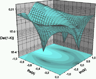
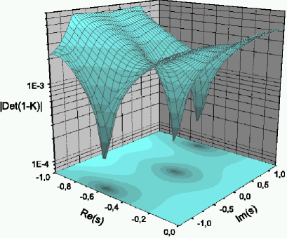
Figure 4: Plots of $|Det(\openone-K)|$ for pseudoscalar (left panel) and scalar (right panel) channels as a function of complex $s$ showing the location of zeroes in the near timelike region ($\overline{u}u$ case).

Turning now to the solutions of Eqs. (LABEL:eq:4pt3) we start with spacelike $l^{2}$ and show typical results for the $\overline{u}u$ flavor combination with $s=1+\imath$. As previously discussed, the $t$-dependence of the solution is removed by setting the seed term to $1/\sqrt{2}$ such that the zeroth Chebyshev as $l^{2}\rightarrow\infty$ tends to unity ($-3$) for the diquark (mesonic) components. We note that for general complex $s$ the Chebyshev moments of the amplitudes will be complex. We show both the real and imaginary parts of the Chebyshev moments of the diquark $G^{n,1}$ component in Fig. 5. Clearly seen is that the real part of the zeroth Chebyshev dominates primarily because of the seed terms in Eqs. (LABEL:eq:4pt3). Essentially the 4-pt function away from resonance positions shows its tree-level form. Furthermore, the diquark components do not have a resonance in either the spacelike or near timelike regions and one might conclude that $G^{n}$ could be well approximated by its tree-level term entirely; this will turn out not to be the case. The mesonic components for this value of $s$ display the same behavior as their diquark counterparts. However, the mesonic sector does have resonances where the subleading Chebyshev structure and the deviation from the tree-level form become important.

     

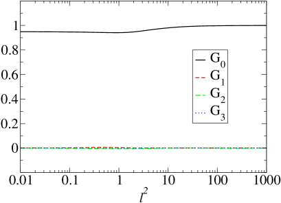
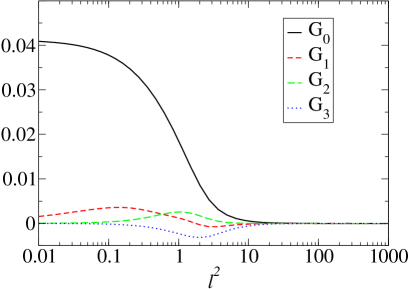
Figure 5: Real and imaginary (left and right panels respectively) parts of the Chebyshev moments, $G_{i}^{n,1}(s=1+\imath,t,l^{2})$ for real $l^{2}$.

We display the real parts of the zeroth Chebyshev amplitudes of the diquark and meson amplitudes as functions of spacelike $l^{2}$ for $s=1+\imath$ in Fig. 6. This plot specifies the behavior of these functions away from resonance. As $l^{2}$ increases the scalar and pseudoscalar, vector and axialvector functions converge to the same values. This is because the difference between the channels (at this level of approximation) is the sign of the factor $s_{1}s_{2}$ in the kernel, which as $l^{2}\rightarrow\infty$ rapidly vanishes. A comparison of the diquark and mesonic channels reveals that the two have similar shaped curves, though with different amplitudes. This can be attributed to the similarity in the kernels of the two channels.

     

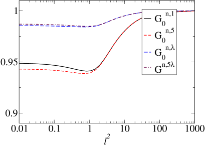
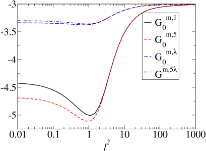
Figure 6: Real parts of the zeroth Chebyshev moment of the diquark and meson (left and right panels, respectively) amplitudes $G_{0}^{(n,m)a}(s=1+\imath,t,l^{2})$ displayed as functions of real $l^{2}$.

It is, furthermore, instructive to plot $G_{0}^{(n,m)a}(s,t,l^{2}=0)$ as a function of real $s$ to highlight the resonance structure (cf. Fig. 7). The diquark correlations show no resonance structure, but crucially do show significant variation with $s$, implying that the tree-level approximation is not reliable for low $s$. The mesonic correlations show resonance structures as expected. It is tempting to approximate these curves by a simple $1/(s+m^{2})$ shape, but closer inspection reveals that there they are indeed more complicated. This is an important point to note since the deviations from the pole term are significant.

     

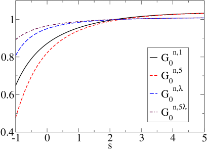
Figure 7: Zeroth Chebyshev moments of the diquark and meson (left and right panels, respectively) amplitudes $G_{0}^{(n,m)a}(s,t,l^{2}=0)$ plotted as functions of real $s$.

Finally, we show the functions $G_{i}^{(n,m)a}(s,t,l^{2})$ for the case of complex $l^{2}$. Recall that in the kernel we need the amplitude for $l^{2}=(k+q/2\pm P/4)^{2}$, where $k,q$ are integration variables, $P^{2}=-M^{2}$, while $M$ is the complex mass of the meson under consideration. The factor $P/4$ does, however, mean that the deviation from the spacelike axis will only be slight. A consideration of the exponential interaction shows that the functions will be varying most significantly in the timelike and imaginary directions. Thus it is important that these deviations are taken into account, if only to assess their relevance to the final results. We show $G_{0}^{m,5}(s=1+\imath,t,l^{2})$ (the leading Chebyshev moment of the $\pi$) for complex $l^{2}$ in the vicinity of zero in Fig. 8. It is seen is that the functions vary smoothly and – as expected – the variation becomes larger when progressing into the complex region.

     

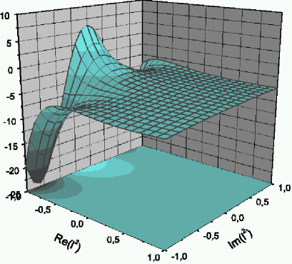
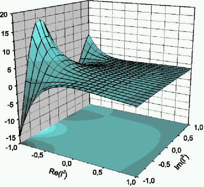
Figure 8: Real and imaginary (left and right panels, respectively) parts of the zeroth Chebyshev moments of the $\pi$ amplitude $G_{0}^{m,5}(s=1+\imath,t,l^{2})$ plotted as functions of complex $l^{2}$ in the vicinity of $l^{2}=0$.

V Summary and Conclusions

In this work, a proposed approximate form for the connected four-point quark-antiquark Green’s function ($G^{4}$) has been studied. The motivation for the study is an extension of the conventional Schwinger–Dyson – Bethe–Salpeter scheme to explore unquenching effects in the light meson sector. The expression for the approximated four-point quark-antiquark Green’s function has been derived and shown to be consistent with asymptotic limits. Furthermore, it reproduces the leading structure of the ladder Bethe–Salpeter equation for the (lightest) pseudoscalar mesons. The resulting equations have been solved numerically and typical results presented for both real and complex momenta.

Most of the approximations employed in this work have been made for heuristic purposes and should be investigated in more detail in subsequent work. Nevertheless, our calculations demonstrate that the scheme proposed already gives acceptable results for the light meson sector and excludes resonances in the diquark channel. Clearly these initial results provide a basis for the study of dynamical meson decay and possible multiquark structures.

References

- (1) M. Golterman, and Y. Shamir, [arXiv:hep-lat/0404001]; J. Smit, Nucl. Phys. Proc. Suppl. 17 (1990) 3; D. N. Petcher, [arXiv:hep-lat/9301015]; M. Golterman, Nucl. Phys. Proc. Suppl. 94 (2001) 189, [arXiv:hep-lat/0011027]; J. W. Negele et al., Nucl. Phys. Proc. Suppl. 128 (2004) 170, [arXiv:hep-lat/0404005]; K. Schilling, H. Neff, and T. Lippert, [arXiv:hep-lat/0401005].
- (2) P. Maris, and C. D. Roberts, Int. J. Mod. Phys. E12 (2003) 297, [arXiv:nucl-th/0301049].
- (3) C. D. Roberts and S. M. Schmidt, Prog. Part. Nucl. Phys. 45 (2000) S1, [arXiv:nucl-th/0005064].
- (4) R. Alkofer, and L. v. Smekal, Phys. Rep. 353 (2001) 281, [arXiv:hep-ph/0007355].
- (5) C. D. Roberts, and A. G. Williams, Prog. Part. Nucl. Phys. 33 (1994) 477, [arXiv:hep-ph/9403224].
- (6) H.J. Munczek, and A.M. Nemirovsky, Phys. Rev. D28 (1983) 181.
- (7) P. Jain, and H. J. Munczek, Phys. Rev. D48 (1993) 5403; H. J. Munczek, and P. Jain, Phys. Rev. D46 (1991) 438; P. Jain, and H. J. Munczek, Phys. Rev. D44 (1991) 1873.
- (8) C. J. Burden, L. Qian, C. D. Roberts, P. C. Tandy, M. J. Thomson, Phys. Rev. C55 (1997) 2649, [arXiv:nucl-th/9605027].
- (9) P. Maris, C. D. Roberts, and P. C. Tandy, Phys. Lett. B420 (1998) 267, [arXiv:nucl-th/9707003].
- (10) R. Delbourgo, and M. D. Scadron, J. Phys. G5 (1979), 1621.
- (11) P. Maris, and P. C. Tandy, Phys. Rev. C60 (1999) 055214, [arXiv:nucl-th/9905056].
- (12) R. Alkofer, P. Watson, and H. Weigel, Phys. Rev. D65 (2002) 094026, [arXiv:hep-ph/0202053].
- (13) P. Maris, and P. C. Tandy, Phys. Rev. C65 (2002) 045211, [arXiv:nucl-th/0201017].
- (14) P. Maris, and P. C. Tandy, Phys. Rev. C61 (2000) 045202, [arXiv:nucl-th/9910033].
- (15) M. S. Bhagwat, M. A. Pichowsky, C. D. Roberts, and P. C. Tandy, Phys. Rev. C68 (2003) 015203, [arXiv:nucl-th/0304003].
- (16) A. Bender, C. D. Roberts, and L. v. Smekal, Phys. Lett. B380 (1996) 7, [arXiv:nucl-th/9602012].
- (17) A. Bender, W. Detmold, C. D. Roberts, and A. W. Thomas, Phys. Rev. C65 (2002) 065203, [arXiv:nucl-th/0202082].
- (18) P. Watson, W. Cassing, and P. C. Tandy, to be published.
- (19) D. Jarecke, P. Maris, and P. C. Tandy, Phys. Rev. C67 (2003) 035202, [arXiv:nucl-th/0208019].
- (20) M. R. Pennington, [arXiv:hep-ph/0309228].
- (21) N. Nakanishi, Supp. Prog. Theo. Phys. 43 (1969) 1.
- (22) D. Kekez, D. Klabucar, and M. D. Scadron, J. Phys. G26 (2000) 1335, [arXiv:hep-ph/0003234].
- (23) J. Kogut, and L. Susskind, Phys. Rev. D10 (1974) 3468.
- (24) M. D. Scadron, G. Rupp, F. Kleefeld, and E. v. Beveren, Phys. Rev. D69 (2004) 014010; erratum-ibid. D69 (2004) 059901, [arXiv:hep-ph/0309109].
- (25) N. A. Törnqvist, ”The lightest scalar nonet”, in Proc. ”Chiral Fluctuations in Hadronic Matter” workshop, Orsay, 16-20 Sept. 2001, p267, edited Z. Aouissat et al., [arXiv:hep-ph/0201171].
- (26) R. L. Jaffe, Phys. Rev. D15 (1977) 267.
- (27) D. Black, A. H. Fariborz, S. Moussa, S. Nasri, and J. Schechter, Phys. Rev. D64 (2001) 014031, [arXiv:hep-ph/0012278].
- (28) F. E. Close, and N. A. Törnqvist, J. Phys. G28 (2002) R249, [arXiv:hep-ph/0204205].
- (29) P.C. Tandy, Prog. Part. Nucl. Phys. 39 (1997) 117, [arXiv:nucl-th/9705018].
- (30) M. S. Bhagwat, M. A. Pichowsky, and P. C. Tandy, [arXiv:hep-ph/0212276].
- (31) P. Cvitanovic, Phys. Rev. D14 (1976) 1536.
- (32) R. T. Cahill, J. Praschifka, and C. J. Burden, Aust. J. Phys. 42 (1989) 161.