SLAC–PUB–10457

May 2004

hep-ph/0405242

Composite Vector Mesons from QCD to the Little Higgs
Maurizio Piai¹, Aaron Pierce^2,3, Jay G. Wacker³

1. Department of Physics

Yale University

New Haven, CT 06520

2. Theory Group

Stanford Linear Accelerator Center

Menlo Park, CA 94025

3. Institute for Theoretical Physics

Stanford University

Stanford, CA 94305

We review how the $\rho$ meson can be modeled in an effective theory and discuss the implications of applying this approach to heavier spin-one resonances. Georgi’s vector limit is explored, and its relationship to locality in a deconstructed extra-dimension is discussed. We then apply the formalism for $\rho$’s to strongly coupled theories of electroweak symmetry breaking, studying the lightest spin-one techni-$\rho$ resonances. Understanding these new particles in Little Higgs models can shed light on previously incalculable, ultraviolet sensitive physics, including the mass of the Higgs boson.

1 Introduction

Little Higgs models have recently rekindled interest in theories where the Higgs is a pseudo-Nambu-Goldstone boson (PNGB)[1, 2, 3, 4]. These models can naturally be ultraviolet-completed into theories of strong dynamics, although linear sigma model UV completions are possible. If completed into a theory of strong dynamics, the PNGBs arise when the gauge dynamics at a scale $\Lambda\sim$ 10 TeV breaks global chiral symmetries of the theory. These PNGBs are not the only states associated with the strong dynamics – a host of resonances are expected near the scale of strong coupling. The energy at the Large Hadron Collider (LHC) will be insufficient to directly explore the constituents of the strong dynamics; therefore, the question of more immediate interest is how to describe the low-lying states of the strong dynamics. It is challenging to study the phenomenology of the theory in this regime because the dynamics are strongly coupled.

The same situation exists in QCD: the chiral Lagrangian accurately models the interactions of the pions at the lowest energies; perturbation theory is a powerful tool at high energies, but it is difficult to discuss the interactions of the QCD resonances near the strong coupling scale, such as the $\rho$. Historically, a variety of techniques have been employed to investigate these resonances, including current algebra, QCD sum rules, dispersion relations, and hidden local symmetry. In this paper, we first discuss the $\rho$ mesons of QCD; the lessons learned are used in the subsequent treatment of techni-$\rho$ mesons in Little Higgs theories.

We use hidden local symmetry because this technique is valid at low energies and small $Q^{2}$, precisely the regime in which we are interested. In the hidden local symmetry approach, one writes an effective Lagrangian including the $\rho$ mesons, analogous to the traditional chiral Lagrangian written for the pions [5]. Gauge symmetries are useful for describing light vector mesons and can be used to constrain the interactions of the $\rho$ [6]. The lightness of the $\rho$ (relative to $4\pi f_{\pi}\equiv\Lambda$) is crucial to success in this program. While the separation between $m_{\rho}$ and $\Lambda$ is not incredibly large, it is enough to be predictive. These predictions are qualitatively correct and, perhaps surprisingly, quantitatively not far from the experimentally measured values.

Another asset of the language of hidden local symmetry is that it clearly illuminates the possibility of an enhanced symmetry for QCD, reflected in a particular value of the $\rho$-pion coupling. This symmetry point is essentially the “vector limit” discussed in [6], and reviewed in our Sec. 2.2. As we will discuss, QCD is not too far from realizing this enhanced symmetry. Reference [7] showed that a theory comprised of gauge groups and bi-fundamental fields can be mapped directly on to a description of a physical extra dimension. In particular, notions that are traditionally associated with a physical dimension, such as locality, can be preserved in the theory space description. We find that the vector limit is closely related to locality in theory space.

Including the lightest spin-one resonances in the effective theory allows us to address questions of how high energy physics affects the PNGBs. In particular, we can examine the unitarization of the PNGB scattering. We also find that the incorporating the techni-$\rho$’s into the effective field theory associated with electroweak symmetry breaking (EWSB) can shed light on previously incalculable quantities in Little Higgs models.

The organization of the paper is as follows. In Sec. 2 we review the couplings of the $\rho$ in the QCD chiral Lagrangian. This gives a well-understood example for the hidden local symmetry approach and motivates our discussion of techni-$\rho$’s and their properties in more general theories of strong dynamics. For our discussion of $\rho$’s in QCD, we draw heavily upon the paper [6]. In our discussion of the weak-scale strong dynamics, we will emphasize the potential utility of (techni-)$\rho$’s in regulating quadratic divergences. To motivate this point, we again turn towards QCD. In Sec. 2.2, we introduce the vector limit of QCD. In this limit, the $\rho$’s regulate the quadratic divergence in the charged pion mass that arises from QED loops [8]. Having laid a foundation with our discussion of the QCD $\rho$ meson, we then turn towards a discussion of the techni-$\rho$ and its couplings. We explain how techni-$\rho$ mesons can analogously soften quadratic divergences in Little Higgs models in Sec. 3. This allows us to calculate previously UV-sensitive quantities, including the Higgs boson mass in the Littlest Higgs model. We also note that the inclusion of techni-$\rho$’s can have important consequences for studying vacuum alignment: in the vector limit, the vacuum of the $SU(6)/Sp(6)$ theory is unstable. In Sec. 4, we discuss how unitarity is modified by incorporating light resonances. We argue that the low scale of unitarity violation in theories with many PNGBs is likely a signal of light scalar resonances rather than vector modes.

2 The Hidden Locality of Vector Mesons In QCD

We first review the coupling of vector mesons in two flavor QCD in the limit of vanishing quark masses[6]. The chiral Lagrangian that describes the coupling of the $\rho$ to the light pions will only depend on a handful of parameters. Among these is a parameter that vanishes in Georgi’s vector limit. In this limit, the leading cut-off sensitivity to $m_{\pi^{\pm}}^{2}-m_{\pi^{0}}^{2}$ also vanishes, leaving a residual piece that is not sensitive to cut-off uncertainties. We spend this section exploring this example before moving to TeV scale physics in the next section.

In QCD with two flavors, $\psi_{L}^{i}$ and $\psi_{R}{}_{j}$ ($i,j$ = 1,2), there is a global $SU(2)_{L}\times SU(2)_{R}$ flavor symmetry that rotates two quarks amongst themselves:

$$\psi_{L}\rightarrow g_{L}\psi_{L},\hskip 36.135pt\psi_{R}\rightarrow g_{R}\psi_{R}.$$ (2.1)

After the QCD gauge coupling goes strong, this chiral symmetry is broken, and the quarks form a condensate

$$\langle\psi^{i}_{L}\psi_{R}{}_{j}\rangle\sim 4\pi f^{3}\Sigma^{i}_{j}.$$ (2.2)

Here $\Sigma$ parameterizes the QCD pions, which are Goldstone bosons of the broken global symmetry

$$SU(2)_{L}\,\times\,SU(2)_{R}\,\longrightarrow\,SU(2)_{V}\,,$$ (2.3)

where $SU(2)_{V}$ is the unbroken isospin symmetry. Under this symmetry, the transformation of the Goldstone boson field is

$$\Sigma\rightarrow g_{L}\Sigma g_{R}^{\dagger}.$$ (2.4)

The linearized fluctuations of $\Sigma$ and global symmetry transformations are given by

$$\Sigma\,\equiv\,e^{2i\pi/f}\hskip 43.36243ptg_{L}\equiv e^{i\alpha_{L}},\hskip 28.90755ptg_{R}\equiv e^{i\alpha_{R}}.$$ (2.5)

The linearized $\pi$ field transforms under the global symmetries as:

$$\delta\pi=\frac{f}{2}(\alpha_{L}-\alpha_{R})+\cdots.$$ (2.6)

The vector and axial–vector transformations are distinguished by the relationship between $\alpha_{L}$ and $\alpha_{R}$. For the axial–vector transformation, we have $\alpha_{L}=-\alpha_{R}\equiv\alpha_{A}$, while for the vector transformation, we have $\alpha_{L}=\alpha_{R}\equiv\alpha_{V}$. Then $\delta\pi=f\alpha_{A}$. The quarks are also charged under a weakly gauged group, $U(1)_{EM}$. $U(1)_{EM}$ is contained within $SU(2)_{V}$, and is gauged in the $\tau^{3}$ direction. The symmetry structure of the theory, both global and local, is illustrated in Fig. 1. To leading order, the chiral Lagrangian describing the pions is:

$$\mathcal{L}_{\text{eff}}\,=\,-\frac{1}{4}F_{\mu\nu}^{2}+\frac{f^{2}}{4}\,\mbox{Tr}\,|D_{\mu}\Sigma|^{2}+\cdots,$$ (2.7)

where the covariant derivative is given by

$$D_{\mu}\Sigma=\partial_{\mu}\Sigma+ieA_{\mu}[\tau^{3},\Sigma]\hskip 21.68121pt\text{ with }\mbox{Tr}\,\tau^{a}\tau^{b}=\frac{1}{2}\delta^{ab}.$$ (2.8)

$\Sigma$ transforms like $(2,\bar{2})$ under $SU(2)_{L}\times SU(2)_{R}$. Parity interchanges $SU(2)_{L}\leftrightarrow SU(2)_{R}$ and takes $\Sigma\rightarrow\Sigma^{\dagger}$. Note that the $f$ in Eq. 2.7 can be identified with the pion decay constant, $f_{\pi}=93$ MeV.

2.1 Incorporating the $\rho$

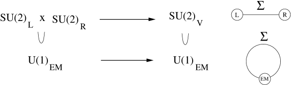
Figure 1: QCD with two flavors has a global $SU(2)_{L}\times SU(2)_{R}$ chiral symmetry, which is broken down to the diagonal $SU(2)_{V}$ (isospin) when the quarks condense. As shown above, the $U(1)_{EM}$ gauge symmetry is contained within $SU(2)_{V}$. We have also shown these symmetries in a “sites and links” theory space representation. The top diagram shows that the quark condensate transforms as a bi-fundamental under $SU(2)_{L}\times SU(2)_{R}$, and breaks this symmetry down to the diagonal. The bottom diagram shows that the quark condensate is an adjoint of the gauged $U(1)_{EM}$.

Now we include the $\rho$ meson in our low energy theory. The lightness of the $\rho$ mesons also motivates a description utilizing a gauge invariance, $SU(2)_{\rho}$. The longitudinal components of the $\rho$ are kept explicit, and the gauge invariance can be used to determine the natural sizes of operators in the effective Lagrangian. Of course this gauge symmetry has no physics in it, and going to the unitary gauge makes this clear. A lucid discussion of this point was given in [6, 9]. We emphasize that it is the lightness of the $\rho$ that constrains its properties– we expect additional operators in the effective Lagrangian proportional to $m_{\rho}/\Lambda$. For example, there are higher derivative operators that can sum into a form-factor that reveals the composite nature of the $\rho$. Upon including the $\rho$ in the chiral Lagrangian, the symmetry structure is enlarged to become:

$$SU(2)_{L}\,\times\,SU(2)_{R}\,\times\,SU(2)_{\rho}\,\longrightarrow\,SU(2)_{V},$$ (2.9)

where the $SU(2)_{\rho}$ symmetry is strongly gauged. This structure is displayed in Fig. 2.

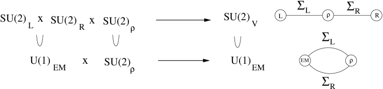
Figure 2: The global (including $g_{\rho}\rightarrow 0$) and gauge symmetry structure of the QCD pions and a typical $\rho$ vector meson. This figure is the analogue of Fig. 1, now with the $\rho$’s included. The “sites and links” diagrams show the global and gauge symmetries under which the $\Sigma_{L}$ and $\Sigma_{R}$ fields transform as bi-fundamentals.

The effective theory, now incorporating both $\pi$’s and $\rho$’s, is

$$\mathcal{L}_{\text{eff}}\, = \,-\frac{1}{4}F_{\mu\nu}^{2}-\frac{1}{2}\mbox{Tr}\,\rho_{\mu\nu}^{2}-\tilde{\kappa}F_{\mu\nu}(\mbox{Tr}\,\tau^{3}\Sigma_{L}\rho^{\mu\nu}\Sigma_{L}^{\dagger}+\mbox{Tr}\,\tau^{3}\Sigma_{R}^{\dagger}\rho^{\mu\nu}\Sigma_{R})$$ (2.10)

$$+\frac{f^{2}}{4}\,\left(\mbox{Tr}\,|D^{\mu}\Sigma_{L}|^{2}+\mbox{Tr}\,|D^{\mu}\Sigma_{R}|^{2}+\,\frac{\kappa}{2}\,\mbox{Tr}\,|D^{\mu}(\Sigma_{L}\Sigma_{R})|^{2}\right)\,+\cdots,$$

where $\tilde{\kappa}$ sets the size of the $\rho-\gamma$ kinetic mixing. This effective action is the result of integrating out all heavier resonances. We refer to the operators multiplied by $\kappa$ and $\tilde{\kappa}$ as “non-local”: in the theory-space description of Fig. 2, these operators involve more than one site, and so are indeed non-local in theory space. For simplicity, we will set $\tilde{\kappa}$ to zero throughout; however, retaining it would be important if our goal were to try to match this theory to experimental QCD. Parity acts on the theory by taking $SU(2)_{L}\leftrightarrow SU(2)_{R}$, leaving $SU(2)_{\rho}$ unchanged, and taking the Goldstone bosons from $\Sigma_{L}\leftrightarrow\Sigma_{R}^{\dagger}.$ We have imposed parity on the Lagrangian in Eq. 2.10. The transformations under the $SU(2)_{L}\times SU(2)_{R}\times SU(2)_{\rho}$ symmetry are:

$$\Sigma_{L}\equiv\exp(2i\pi_{L}/f)\sim(2,\bar{2},1); \Sigma_{L}\rightarrow g_{L}\Sigma_{L}g_{\rho}^{\dagger},$$

$$\Sigma_{R}\equiv\exp(2i\pi_{R}/f)\sim\,(1,2,\bar{2}); \Sigma_{R}\rightarrow g_{\rho}\Sigma_{R}g_{R}^{\dagger},$$

$$\Sigma_{L}\Sigma_{R}\equiv\exp(2i(\pi_{L}+\pi_{R})/f)\sim\,(2,1,\bar{2}); \Sigma_{L}\Sigma_{R}\rightarrow g_{L}\Sigma_{L}\Sigma_{R}g_{R}^{\dagger},$$ (2.11)

where $g_{L}$, $g_{R}$ and $g_{\rho}$ are independent $SU(2)$ transformations. The covariant derivatives that appear in Eq. 2.10 are

$$D_{\mu}\Sigma_{L} = \partial_{\mu}\Sigma_{L}+ie_{0}A_{\mu}\tau^{3}\,\Sigma_{L}-ig_{\rho}\Sigma_{L}\,\vec{\tau}\cdot\vec{\rho}_{\mu},$$

$$D_{\mu}\Sigma_{R} = \partial_{\mu}\Sigma_{R}+ig_{\rho}\vec{\tau}\cdot\vec{\rho}_{\mu}\,\Sigma_{R}-ie_{0}\Sigma_{R}\,A_{\mu}\tau^{3},$$

$$D_{\mu}\Sigma_{L}\Sigma_{R} = \partial_{\mu}\Sigma_{L}\Sigma_{R}+ie_{0}A_{\mu}[\tau^{3},\Sigma_{L}\Sigma_{R}].$$ (2.12)

Here, $A_{\mu}$ is the vector field that mixes with the $\rho^{3}$. Proceeding to the mass eigenbasis, we find a zero eigenvalue (the photon) and a massive eigenvalue (the physical $\rho$).

It is possible to go to the unitary gauge where the new degrees of freedom become the longitudinal components of the $\rho$. This gauge is convenient because the physical couplings of the $\rho$ are manifest; however, their natural sizes are more difficult to infer. We can determine this gauge by examining the Goldstone-$\rho$ mixing. Ignoring the weakly gauged $U(1)_{EM}$, the mixing is given by

$$\mathcal{L}_{\rho\pi}=g_{\rho}f\,\mbox{Tr}\,\rho_{\mu}\left(\partial^{\mu}\pi_{L}-\partial^{\mu}\pi_{R}\right).$$ (2.13)

Thus, the physical pion, $\pi$, and the Goldstone eaten by the $\rho$, denoted by $\xi$, are related to the gauge eigenstates by

$$\pi=N_{\pi}^{-1}(\pi_{L}+\pi_{R}),\hskip 36.135pt\xi=N_{\xi}^{-1}(\pi_{L}-\pi_{R}),$$ (2.14)

where $N_{\pi}$ and $N_{\xi}$ are constants determined by the requirement that the fields be canonically normalized. Unitary gauge is defined by $\xi=0$.

The gauge and global transformations are

$$g_{L}=e^{i\alpha_{L}},\hskip 36.135ptg_{\rho}=e^{i\alpha_{\rho}},\hskip 36.135ptg_{R}=e^{i\alpha_{R}},$$ (2.15)

and act upon the linearized fields as

$$\delta\pi_{L}=\frac{f}{2}\Big{(}\alpha_{L}-\alpha_{\rho}\Big{)},\hskip 36.135pt\delta\pi_{R}=\frac{f}{2}\Big{(}\alpha_{\rho}-\alpha_{R}\Big{)}.$$ (2.16)

The vector and axial vector transformations should preserve unitary gauge. Therefore, we can parameterize the transformations by the two global ones and the orthogonal one, which can be used to go to unitary gauge:

$$\rm{Vector:}\hskip 7.22743pt\alpha_{L}=\alpha_{\rho}=\alpha_{R}\equiv\alpha_{V};\hskip 36.135pt\rm{Axial:}\hskip 7.22743pt\alpha_{L}=-\alpha_{R}\equiv\alpha_{A},\hskip 14.45377pt\alpha_{\rho}=0.$$ (2.17)

The leading kinetic term for the pions is given by

$$\mathcal{L}_{(\partial\pi)^{2}} = \mbox{Tr}\,(\partial\pi_{L})^{2}+\mbox{Tr}\,(\partial\pi_{L})^{2}+\kappa\mbox{Tr}\,(\partial(\pi_{L}+\pi_{R}))^{2};$$ (2.18)

$$= \frac{1}{2}N_{\pi}^{2}(1+\kappa)\mbox{Tr}\,(\partial\pi)^{2}+\frac{1}{2}N_{\xi}^{2}\mbox{Tr}\,(\partial\xi)^{2}=\mbox{Tr}\,(\partial\pi)^{2}+\mbox{Tr}\,(\partial\xi)^{2},$$

meaning that the normalization constants are given by

$$N_{\pi}^{-2}=\frac{1+\kappa}{2},\hskip 36.135ptN_{\xi}^{-2}=\frac{1}{2}.$$ (2.19)

Under an axial transformation

$$\delta\pi=N^{-1}_{\pi}f\alpha_{A},\hskip 36.135pt\delta\xi=0.$$ (2.20)

Acting on Eq. (2.18), we find:

$$\delta\mathcal{L}_{(\partial\pi)^{2}}=2N^{-1}_{\pi}f\mbox{Tr}\,\partial\pi\partial\alpha_{A}=2f_{\pi}\mbox{Tr}\,\partial\pi\partial\alpha_{A}.$$ (2.21)

This allows us to identify

$$f_{\pi}=\sqrt{\frac{1+\kappa}{2}}f.$$ (2.22)

The only a priori constraint on $\kappa$ is that $\kappa>-1$, so that the physical $\pi$ has a positive kinetic term. At this point we can diagonalize the mass mixing with an orthogonal transformation

$$A_{\text{Phys}} = \cos\theta\hat{A}+\sin\theta\rho^{3},\hskip 36.135pt\rho^{3}_{\text{Phys}}=-\sin\theta\hat{A}+\cos\theta\rho^{3}.$$ (2.23)

where the angles and electro-magnetic gauge coupling are given by

$$e^{-2}=e_{0}^{-2}+g_{\rho}^{-2},\hskip 21.68121pt\sin\theta\equiv\frac{e}{g_{\rho}}.$$ (2.24)

So the couplings of the physical $\rho$ and photon to the electro-magnetic current, $j_{EM}$, are given by

$$\mathcal{L}_{j\,\gamma}=e\,j_{\mu\;EM}\Big{[}A^{\mu}_{\text{Phys}}-\tan\theta\rho^{3\,\mu}_{\text{Phys}}\Big{]},$$ (2.25)

while the masses of the $\rho$ mesons are

$$m^{2}_{\rho^{\pm}}=\frac{g^{2}_{\rho}f^{2}_{\pi}}{1+\kappa},\hskip 14.45377ptm^{2}_{\rho^{0}}=\frac{m^{2}_{\rho^{\pm}}}{\cos^{2}\theta}.\hskip 21.68121pt$$ (2.26)

For large $g_{\rho}$, the difference between the masses of the charged and neutral $\rho$ mesons can be expanded as

$$\frac{m^{2}_{\rho^{0}}}{m^{2}_{\rho^{\pm}}}\approx\Big{(}1+\frac{e^{2}}{g_{\rho}^{2}}\Big{)}.$$ (2.27)

The experimental limits on the mass splittings are bounded to be

$$m_{\rho^{0}}-m_{\rho^{\pm}}\,\raise 1.29167pt\hbox{$<$\kern-7.5pt\lower 4.30554pt\hbox{$\sim$}}\,1\text{ MeV}\Rightarrow 1-\frac{m_{\rho^{0}}}{m_{\rho^{\pm}}}\leq 3\times 10^{-3}.$$ (2.28)

For small $\tilde{\kappa}$, the mass splittings place a limit on $g_{\rho}\simeq 4\pi/\sqrt{3}$. Then, using $f_{\pi}\simeq 93\text{ MeV}$ and $m_{\rho}\simeq 770\text{ MeV}$, we find $\kappa\simeq\frac{1}{3}$ in QCD. There are other determinations of $\kappa$ that give roughly the same answer, e.g. using the KSFR relation for the $\rho\rightarrow\pi\pi$ decay width [11].

For future reference we calculate the $\rho$’s coupling to the isospin current of the $\pi$’s

$$\mathcal{L}_{\text{int}}=gj^{a}_{\mu}\rho_{a}^{\pm}\hskip 36.135ptj^{a}_{\mu}=\mbox{Tr}\,\tau^{a}[\partial_{\mu}\pi,\pi]\hskip 21.68121ptg=\frac{g_{\rho}}{1+\kappa}.$$ (2.29)

2.2 Georgi’s Vector Limit

In this section, we discuss an enhanced symmetry of the strong dynamics known as the vector limit. When this symmetry is exact, the $\rho$ meson acts to cut off the one loop gauge (QED) quadratic divergence of the charged pion mass. As we will discuss, a similar enhanced symmetry is possible in general theories of strong dynamics, including theories at the weak scale.

Starting from Eq. 2.10, one can compute the contribution of the photon to the mass of the charged pion with the Coleman-Weinberg potential [12]. At one loop one finds:

$$\delta m^{2}_{\pi^{\pm}}=\frac{3e^{2}}{16\pi^{2}(1+\kappa)}\Big{(}\frac{\kappa\Lambda^{2}}{\cos^{2}\theta}+m^{2}_{\rho^{0}}\log\Lambda^{2}+\cdots\Big{)}.$$ (2.30)

The term “$\cdots$” includes a logarithmically divergent piece that is proportional to $\kappa\tan^{2}\theta$, which is numerically very small. For the special case of $\kappa$=0, the one loop quadratic divergence is absent, and the counter-term from high energy physics is only necessary to cancel two loop quadratic divergences. The degree to which the one-loop logarithmic divergence is larger than the two-loop quadratic divergence is the degree to which the $\delta m_{\pi^{\pm}}^{2}$ is calculable. When $\kappa\neq 0$, a one loop quadratic divergence remains.

This can be explained by studying the symmetry structure of the Lagrangian. For the QCD Lagrangian of Eq. 2.10, in the limit that $g_{\rho}$ and $e_{0}$ vanish, the global symmetry of the theory is as shown in Fig. 3. Note if $\kappa=0$, this Lagrangian would allow independent transformations of the form $\Sigma_{L}\rightarrow\Sigma_{L}U_{L}$ and $\Sigma_{R}\rightarrow U_{R}\Sigma_{R}$. A non-zero $\kappa$ forces $U_{L}=U_{R}$. We refer to this limit of enhanced symmetry as the vector limit.

The global symmetry of the vector limit is

$$SU(2)_{L}\times SU(2)_{R}\times SU(2)_{\rho_{L}}\times SU(2)_{\rho_{R}},$$ (2.31)

as shown in Fig. 3. The symmetry structure translates into a constraint on the coupling of the $\rho$ to the pions.

With $\kappa=0$, this theory has become a two site, two link, “theory space” model. The $\rho$ cuts off the quadratic divergence to the charged pion mass, just as in traditional Little Higgs theories, where vector bosons come in to cut off the gauge quadratic divergences to the Higgs boson mass. The possibility that $\rho$’s could cut-off quadratic divergences to pseudo-Goldstone bosons was previously noted, see [13].

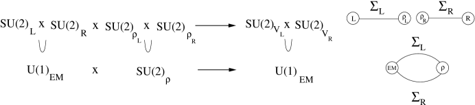
Figure 3: The global (including $g_{\rho}\rightarrow 0$) and gauge symmetry structure of the QCD pions and $\rho$ vector meson in the vector limit ($\kappa\rightarrow 0$). While the vector limit does not change the gauge symmetry structure of the theory, it does change the global symmetry. This translates into a relation between $m_{\rho}$, $g_{\rho}$ and $f_{\pi}$.

2.3 Higher Modes

So far we have limited discussion to the $\rho$ meson, the lightest vector resonance. It is natural to attempt to extend the methods employed above to more massive spin-one resonances, such as the $a_{1}$. However, our technology crucially relies on the lightness of the modes relative to the scale of strong coupling. As the resonances become heavier, the constraint of gauge invariance on their interactions is weakened, and the validity of the effective Lagrangian becomes more precarious.

In QCD the $a_{1}$ might already be too massive to be well-described by hidden local symmetry, other theories with strong dynamics may have a wider range of states to which hidden local symmetry can be applied. For instance, the number of light resonances (those with mass $\,\raise 1.29167pt\hbox{$<$\kern-7.5pt\lower 4.30554pt\hbox{$\sim$}}\,4\pi f_{\pi}$) scales with the number of colors of the confining theory, $N_{c}$; so for large $N_{c}$ QCD, there are many light vector resonances and therefore more modes can be faithfully studied. Likewise, in applications to EWSB, the $N_{c}$ of the UV completion may be larger than three, allowing for more light copies of the $\rho$ and $a_{1}$ to be described within an effective theory.

In [10, 14], an infinite number of sites was considered to model QCD. However, as the number of sites increases, to keep the interactions of the $\rho$’s from becoming weak, the gauge coupling at each individual site must increase. The result, as shown in [15], is that if too many sites are used in the effective theory, the radiative corrections to operators non-local in the deconstructed dimensions grow exponentially large except in special supersymmetric examples. Since locality is crucial to interpreting the theory as extra-dimensional, the large non-local radiative corrections to the effective action calls into question the whole extra-dimensional interpretation. In QCD, the physical coupling of the $\rho$ is strong. At best a few sites can be included while avoiding this pitfall. If the physical coupling of the $\rho$ were weaker, more sites could be consistently included without encountering this difficulty.

Despite the caveats enumerated here, we will first study the theory space representation of the $a_{1}$ in QCD. Our ultimate goal is studying light resonances in a more general setting, but the $a_{1}$ in QCD gives a familiar example.

2.3.1 The $a_{1}$ in QCD and the Generalized Vector Limit

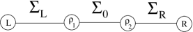
Figure 4: Chiral Lagrangian with the lightest $a_{1}$ modeled.

In QCD the heavier spin-one resonances can be modeled by incorporating new gauge symmetries in the middle of the theory space. This construction is equivalent to the construction in [5] and is much as [10] attempted in a more ambitious manner.

With an additional strongly gauged field, we can model the interactions of the $a_{1}$ (See Fig. 4). The Lagrangian becomes

$$\mathcal{L} = -\frac{1}{2}\mbox{Tr}\,\rho_{1\,\mu\nu}^{2}-\frac{1}{2}\mbox{Tr}\,\rho_{2\,\mu\nu}^{2}+\frac{f^{2}}{4}\Big{(}|\mbox{Tr}\,D_{\mu}\Sigma_{L}|^{2}+c^{2}|\mbox{Tr}\,D_{\mu}\Sigma_{0}|^{2}+|\mbox{Tr}\,D_{\mu}\Sigma_{R}|^{2}$$ (2.32)

$$+\kappa|\mbox{Tr}\,D_{\mu}\Sigma_{L}\Sigma_{0}|^{2}+\kappa|\mbox{Tr}\,D_{\mu}\Sigma_{0}\Sigma_{R}|^{2}+\kappa^{\prime}|\mbox{Tr}\,\partial_{\mu}\Sigma_{L}\Sigma_{0}\Sigma_{R}|^{2}\Big{)},$$

where we are neglecting $U(1)_{EM}$ and also the various kinetic mixings for simplicity. Both $\rho_{1}$ and $\rho_{2}$ have the same gauge coupling, $\tilde{g}_{\rho}$. There is another parameter, $c$, that is a priori undetermined. The linearized fluctuations of the fields are given by

$$\Sigma_{L}=\exp\Big{(}\frac{2i}{f}\pi_{L}\Big{)},\hskip 36.135pt\Sigma_{0}=\exp\Big{(}\frac{2i}{cf}\pi_{0}\Big{)},\hskip 36.135pt\Sigma_{R}=\exp\Big{(}\frac{2i}{f}\pi_{R}\Big{)}.$$ (2.33)

When modeling the $\rho$, we had to introduce a single non-locality parameter, $\kappa$. Here we have a pair: $\kappa$ and $\kappa^{\prime}$. A parity transformation interchanges $SU(2)_{L}\leftrightarrow SU(2)_{R}$. Under this parity, there is an even field, the $\rho$, and and odd field, the $a_{1}$. Note that the two terms with coefficient $\kappa$ are set equal by this parity.

The masses of the vector mesons are

$$m^{2}_{\rho}=\frac{1+\kappa}{4}g^{2}_{\rho}f^{2},\hskip 36.135ptm^{2}_{a_{1}}=\frac{1+2c^{2}+\kappa}{4}g^{2}_{\rho}f^{2}.$$ (2.34)

Note that the $a_{1}$ is always heavier than the $\rho$. Setting $c=1$ and $\kappa=\kappa^{\prime}=0$, the spectrum in the vector limit is $m_{\rho}^{2}=g_{\rho}^{2}f_{\pi}^{2}$ and $m_{a_{1}}=\sqrt{3}m_{\rho}$. While this prediction does differ from the value predicted by QCD sum rules, $m_{a_{1}}=\sqrt{2}m_{\rho}$, it is not that far from the the experimental relation $m_{a_{1}}/m_{\rho}\simeq 1.65$.

In the limit where all of the gauge couplings, $\kappa$ and $\kappa^{\prime}$ vanish, there are enhanced symmetries much like those in Georgi’s vector limit. When the generalized vector limit holds, the global symmetry of the theory is

$$SU(2)_{L}\times SU(2)_{\rho_{1}}\times SU(2)_{\rho_{2}}\times SU(2)_{R}\rightarrow SU(2)_{L}^{3}\times SU(2)_{R}^{3}.$$ (2.35)

Restoring the gauge couplings while keeping $\kappa$ set to zero gives a finite Coleman-Weinberg potential because it requires $e_{0}$, $g_{\rho_{1}}$, and $g_{\rho_{2}}$ couplings to communicate sufficient chiral symmetry breaking to the effective Lagrangian:

$$\delta m^{2}_{\pi^{\pm}}\sim\frac{3e^{2}}{16\pi^{2}}m_{\rho}^{2}\log\frac{m_{a_{1}}^{2}}{m_{\rho}^{2}}.$$ (2.36)

In this limit, the $\rho$ and the $a_{1}$ cut off both the quadratic and logarithmic divergences from gauge interactions.

2.4 Effects of Higher Modes on the Vector Limit

We have argued that the $\kappa\rightarrow 0$ limit is of particular interest, partly because the quadratic divergences vanish in this limit. We would like to understand how likely this limit is to obtain. To do this, we must understand how higher modes can affect the low-energy Lagrangian. We will see that even if a theory is fundamentally local, integrating out the heavy modes can make the effective theory for the lightest mode appear non-local.

Figure 5: The effect of the $a_{1}$ on the $\pi-\rho$ Lagrangian. The $\pi-\rho-a_{1}$ theory is in the generalized vector limit where all non-local couplings are set to zero. The radiatively induced mass for $\pi^{\pm}$ is finite at one loop. Integrating out the $a_{1}$ at tree level induces a $\kappa$ term, at loop level a compensating counter-term is induced for the $\pi^{\pm}$ mass.

This is not too surprising. For example, a similar phenomenon occurs in a 5D gauge theory on a circle. We can Kaluza-Klein (KK) decompose the vector boson into its ladder spectrum, and form an effective theory by classically integrating out all but the lightest vector boson. In this truncated theory, a computation of the mass for the Wilson loop operator yields an answer quadratically sensitive to the cut-off – an answer far larger than the finite one found by a calculation in the original 5D theory. Locality in the fifth dimension prohibits ultraviolet contributions to the Wilson line operator. Truncating the theory corresponds to placing a hard momentum cut-off in the fifth dimension; when Fourier transformed back to position space, this cut-off induces $x_{5}^{-1}$ correlation functions. Truncating the theory induces non-locality in the fifth dimension; the result is the Wilson loop operator no longer has exponentially small sensitivity to the cutoff. Properly integrating out the tower of KK modes (at the quantum level) induces a counter-term for the Wilson line operator that cancels against the quadratic divergence induced by the interactions of the lightest mode.

To demonstrate how this phenomena occurs in QCD we can return to the formulae of the previous section and classically integrate out the $a_{1}$ resonance. Even when starting in the in the vector limit, a significant deviation from $\kappa=0$ is induced. The Lagrangian of a local $\rho-a_{1}-\pi$ theory is given by

$$L_{\rho\,a_{1}}=\frac{f^{2}}{4}\Big{(}|D_{\mu}\Sigma_{L}|^{2}+c^{2}|D_{\mu}\Sigma_{0}|^{2}+|D_{\mu}\Sigma_{R}|^{2}\Big{)},$$ (2.37)

with gauge couplings $\tilde{g}_{\rho}$ for both of the vector bosons. We start by normalizing $f_{\pi}$ through a calculation similar to the one in Sec. 2.1, which gives [10]

$$f_{\pi}=\frac{f}{\sqrt{2+c^{-2}}}.$$ (2.38)

The two mass eigenvalues are

$$m^{2}_{\rho}=\frac{\tilde{g}_{\rho}^{2}f^{2}}{4}=(2+c^{-2})\frac{\tilde{g}_{\rho}^{2}f_{\pi}^{2}}{4}\hskip 28.90755ptm^{2}_{a_{1}}=\frac{(1+2c^{2})\tilde{g}_{\rho}^{2}f^{2}}{4}=(2+c^{-2})\frac{(1+2c^{2})\tilde{g}_{\rho}^{2}f_{\pi}^{2}}{4}.$$ (2.39)

To relate $\tilde{g}_{\rho}$ to $g_{\rho}$ we consider the coupling of the $\rho$ to the $\pi$ isospin current. We find

$$g=\frac{1+c^{-2}}{2+c^{-2}}\sqrt{2}\tilde{g}_{\rho}.$$ (2.40)

In the non-vector-limit theory with just the $\rho$, the mass of the $\rho$ in terms of the isospin current coupling in Eq. 2.26 and Eq. 2.29

$$m_{\rho}^{2}=(1+\kappa)g^{2}f^{2}_{\pi}$$ (2.41)

where as in the vector-limit theory with the $a_{1}$ the mass of the $\rho$ is given by

$$m_{\rho}^{2}=\frac{(1+\frac{1}{2}c^{-2})^{3}}{(1+c^{-2})^{2}}g^{2}f_{\pi}^{2}$$ (2.42)

keeping the physical quantities $f_{\pi}$ and $g$ fixed, we can vary $c$ and observe how $\kappa$ changes

$$\kappa=\frac{(1+\frac{1}{2}c^{-2})^{3}}{(1+c^{-2})^{2}}-1=-\left(\frac{c^{-2}}{2}\right)\left(\frac{1+\frac{1}{2}c^{-2}-\frac{1}{4}c^{-4}}{(1+c^{-2})^{2}}\right)$$ (2.43)

There are two places where the non-locality becomes small, at $c^{-2}=0$ or at $c^{-2}=1+\sqrt{5}$. At the prior, it is obvious that the theory is local because the middle link has been contracted away and $m_{a_{1}}\rightarrow\infty$, while in the later, it is just a cancellation. The ratio $m_{a_{1}}/m_{\rho}$ suggests that $c^{-2}=0.85$ or $\kappa=-0.15$.

Summarizing, we started with a local theory including the $a_{1}$ resonance, but after integrating out the $a_{1}$, the effective theory that contains only the $\rho$ is apparently non-local (see Fig. 5). This deviation from $\kappa=0$ occurs because the $\rho$ and $\pi$ mix with the $a_{1}$. This deforms the low energy effective action of the $\rho$–$\pi$ system away from a local/nearest neighbor interacting one. After truncating the theory, the counter-term to the $\pi$ mass can be computed in this reduced theory. The counter-term in this case turns out not to violate isospin because the $a_{1}$ does not mix with the photon. The induced counter-term violates does violate $SU(2)$ axial because the longitudinal components of the $a_{1}$ mix with $\pi$. If a $\rho^{\prime}$ was included, then an isospin violating $\kappa$ parameter would be induced.

2.5 Vector Limit Moral

In this section, we explore the meaning of Georgi’s vector limit for QCD, and speculate on the implications for other theories with strong dynamics. It is always possible to use an effective Lagrangian for those modes that are much lighter than the scale of strong coupling. For QCD, this means a Lagrangian for the $\pi$’s and the $\rho$ meson. Keeping the longitudinal components of the $\rho$ explicitly in the effective Lagrangian is useful for constraining their interactions when the mass of the $\rho$ is light compared with the scale of strong coupling. In this gauge, there is a term that breaks more chiral symmetries than the others because it contains more fields. In the vector limit this term vanishes. In Naive Dimensional Analysis (NDA) [16], adding non-linear sigma model fields to any operator does not result in a suppression. Nevertheless, these $\Sigma$-laden terms seem to be small experimentally. So, NDA does not give any reason for the $\kappa$ parameter to be small; insight into the vector limit is beyond the scope of NDA. The suppressed operators with additional $\Sigma$ fields are non-local in theory space. One possible reason for this suppression is that such terms break more chiral symmetries than operators with fewer $\Sigma$ fields; if there is a “cost” associated with the breaking a chiral symmetries, then it would be natural to expect a suppression of these terms.

As shown in the previous section, if there are additional spin-one resonances that mix with the $\rho$ such as the $a_{1}$ then the vector limit is typically spoiled. So if Georgi’s vector limit is to hold, mixing with all heavier modes should be small. A theory space model with many sites incorporates mixing with many spin-one modes ($a_{1}$, $\rho^{\prime}$, $\rho^{\prime\prime}$), even if the spectrum is truncated. To reproduce a model close to the vector limit, we must minimize this mixing. To do this, we write a model with sites and links for only those modes well-constrained by gauge invariance. For QCD, this is probably only the $\rho$. For the vector limit to hold, we must posit that these particles do not have large mixing with the particles whose interactions are unconstrained by gauge invariance.

In the next section we will generalize these statements to other strong coupling theories, such as UV completions of Little Higgs theories. Before doing so, it is useful to recall how several quantities scale with $N_{c}$ [17]. We will use slightly non-standard scalings: we keep $f_{\pi}$ fixed as we vary $N_{c}$. This is useful because $f_{\pi}$ will be an easily measurable quantity and in Little Higgs theories the ratio of $f$ and $v$ will be kept fixed.

The coupling of the $\rho$ scales as

$$g_{\rho}\sim 4\pi/N_{c}^{\frac{1}{2}}.$$ (2.44)

With our results from before, we see that

$$m_{\rho}\propto g_{\rho}f_{\pi}\sim\frac{4\pi f_{\pi}}{N_{c}^{\frac{1}{2}}}.$$ (2.45)

If use $m_{\rho}$ as the cut-off of the low energy theory, then we recover the standard large $N_{c}$ relation that

$$\frac{\Lambda}{f_{\pi}}\simeq\frac{4\pi}{N_{c}^{\frac{1}{2}}}.$$ (2.46)

In general, we will be interested in cases where the $g_{\rho}$, remains large, i.e. the number of colors is not too big.

With these large $N_{c}$ scalings in hand, we can now speculate on how Georgi’s vector limit might extend to other theories. As before, we should write down an effective gauge-invariant Lagrangian for the PNGBs and the light vector resonances. Because the mass of the $\rho$ scales as $1/\sqrt{N_{c}}$, we expect that this Lagrangian will probably contain more than just a single $\rho$ for non-QCD cases. According to NDA, there would be many non-local operators with unsuppressed coefficients. On the other hand, if Georgi’s vector limit is somehow fundamental, and indeed there is a cost for breaking chiral symmetries, we expect that these non-local operators will be suppressed. This dictates that mixing with the higher modes (those not well described in the effective theory) is small.

The fundamental importance of the vector limit can in principle be tested experimentally. If, for example, a EWSB involves a theory at strong coupling, one could check whether or not it was close to the vector limit by exploring the relationship between the $\rho-\pi$ couplings, $m_{\rho}$, and $f_{\pi}$.

3 The Techni-Vector Limit, Vacuum Alignment and Little Higgs Models

Suppose that techni-$\rho$s (henceforth referred to as $\rho$s) are the lightest hadronic states of a multi-TeV confining gauge theory associated with EWSB. How do they couple to the Goldstone bosons? In this section, we show how to include techni-$\rho$’s in the low energy effective theory for composite Higgs models. We also discuss how to define the analog of the vector limit. As a first showcase for this formalism, we investigate the problem of vacuum alignment in these theories. Assuming that the vector limit does obtain, we test some of the results previously obtained using QCD sum rules and essentially reproduce the major results.

We then study the implications of the vector limit for specific Little Higgs models. Assuming there is underlying strong dynamics (at $\sim$10 TeV) which favors the realization of the near-vector limit, it is possible to construct an effective theory in which some of the divergences are softened by these vector bosons. This phenomenon is analogous to the way in which the photon contributions to the charged-pion masses were cut-off by interactions with the $\rho$. In Secs. 3.2.1 and 3.2.2, we give two examples of Little Higgs models where inclusion of techni-$\rho$’s can render previously UV sensitive quantities calculable. First, in the $SU(6)/Sp(6)$ Little Higgs model[4], there is a quadratic divergence in the Coleman-Weinberg potential. The naive sign suggests that the potential is unstable. However, the signs of quadratically divergent quantities are not necessarily to be trusted – with the methods in this paper it is possible to state what features of the ultraviolet completion are necessary to stabilize the effective potential. This is the focus of Sec. 3.2.2. Second, in the Littlest Higgs model[3], the vacuum expectation value (vev) of a electroweak triplet was sensitive to ultraviolet physics. We devote Sec. 3.2.1 to addressing when the vev of the triplet may be smaller than naively expected, as desired by electroweak precision measurements. We are also able to discuss the size of the quartic coupling in this model.

3.1 Coupling Techni-$\rho$’s and Vacuum Alignment

Before proceeding to our specific examples, we discuss how to include techni-$\rho$’s in coset theories of electroweak symmetry breaking. We are particularly interested in models that have the global symmetry structure $SU(N)/SO(N)$ or $SU(N)/Sp(N)$. These symmetry breaking patterns deviate from the QCD-like structure of $[SU(N)\times SU(N)]/SU(N)$ discussed in Section 2, so it is not obvious how to incorporate light vector resonances into the theory. The primary guide is that the vectors should be in a representation of the unbroken global symmetry of the strong dynamics – i.e. $SO(N)$ or $Sp(N)$. We find it convenient to introduce the techni-$\rho$’s in the context of a particular problem: vacuum alignment [18].

In theories of strong dynamics, such as the ones we are considering, vacuum alignment represents an important issue. Consider a strongly gauged group $\mathcal{G}$, with some weakly gauged subgroups $\mathcal{G}_{w}$. As we have discussed, when $\mathcal{G}$ reaches strong coupling, it generically breaks some global symmetries, and may also break some of $\mathcal{G}_{w}$. The issue of vacuum alignment may be succinctly stated as: What subgroup $\mathcal{H}_{w}$ of $\mathcal{G}_{w}$ is left unbroken by the strong dynamics?

Solving the vacuum alignment problem requires the minimization of an effective potential. Unfortunately, this minimization cannot be performed without a knowledge of the bound states of the strongly coupled theory. Reference [19] utilized sum rules [20] to provide a window on this non-perturbative physics. To make progress, they assumed that the signs of spectral integrals could be determined by the lowest lying resonances. In QCD, it is known that this approximation holds: the $\rho$ and the $a_{1}$ largely saturate the vector and axial currents.

Incorporating the techni-$\rho$’s into our effective theory, we too can address vacuum alignment. We simply choose different candidates for $\mathcal{H}_{w}$, and calculate the Coleman-Weinberg effective potential arising from gauge boson and techni-$\rho$ exchange in each case. An instability in the potential means that we have chosen the wrong $\mathcal{H}_{w}$.

At energies beneath $m_{\rho}$, the PNGBs are parameterized as

$$\Sigma=\exp(i\pi/f)\,\Sigma_{0}\,\exp(i\pi^{T}/f),$$ (3.1)

where $\Sigma_{0}$ is the symmetric (anti-symmetric) fermion condensate that breaks $SU(N)$ to $SO(N)$ ($Sp(N)$). The leading action for this theory of Goldstone bosons is

$$\mathcal{L}=\frac{f^{2}}{4}\mbox{Tr}\,|D_{\mu}\Sigma|^{2},$$ (3.2)

where the covariant derivative $D_{\mu}$ is given by

$$D_{\mu}\Sigma=\partial_{\mu}\Sigma+ig_{I}W^{I}_{\mu}(T_{I}\Sigma+\Sigma T_{I}^{T}).$$ (3.3)

Here, the $W^{I}$ are the weakly gauged vector bosons of $\mathcal{G}_{w}$ embedded inside the global $SU(N)$ symmetry. We can study the question of vacuum alignment by examining the effective Coleman-Weinberg potential for the Goldstone bosons. The gauge sector gives rise to quadratic divergences in the potential for the Goldstone bosons:

$$V_{\text{eff}}(\Sigma)\ni\frac{3\Lambda^{2}}{16\pi^{2}}\sum_{I=J}\mathcal{O}_{IJ}$$ (3.4)

with

$$\mathcal{O}_{IJ}(\Sigma)=\frac{f^{2}}{4}\mbox{Tr}\,\Big{[}(g_{I}T_{I}\Sigma+g_{I}\Sigma T_{I}^{T})(g_{J}\Sigma^{\dagger}T_{J}+g_{J}T^{T}\Sigma^{\dagger})\Big{]}.$$ (3.5)

At this point, we cannot say anything definitive about the stability of the effective potential. The quadratic divergence indicates sensitivity to the ultraviolet, and its sign, central to the question of stability, is not to be trusted.

Now we add the techni-$\rho$’s. By taking these vector mesons to be in the adjoint representation of the unbroken chiral symmetry, we can incorporate them into the theory by defining a new multiplet of Goldstone bosons:

$$S\equiv\exp(i\Pi/f)\mbox{ with }\Sigma=S\Sigma_{0}S^{T}.$$ (3.6)

Now $\Pi$ is an adjoint of $SU(N)^{2}/SU(N)$ Goldstone bosons, instead of the $SU(N)/SO(N)$ or $SU(N)/Sp(N)$ Goldstone multiplet we had previously. The longitudinal components of the techni-$\rho$’s have filled out the remainder of the multiplet. $\Sigma$ contains the same set of Goldstone bosons from Eq. 3.1 because the additional Goldstone bosons commute through $\Sigma_{0}$ and cancel. Note that the $SU(N)^{2}$ symmetry of the Lagrangian is broken by the vacuum expectation value $\Sigma_{0}$.

The Lagrangian incorporating the $\rho$’s is given by

$$\mathcal{L}_{T\rho}=f^{2}(\mbox{Tr}\,|D_{\mu}S|^{2}+\frac{\kappa}{4}\mbox{Tr}\,|D_{\mu}\Sigma|^{2}).$$ (3.7)

The covariant derivatives are given by

$$D_{\mu}S = \partial_{\mu}S+ig^{0}_{I}W^{I}_{\mu}T_{I}S+ig_{\rho}ST_{A}\rho_{\mu}^{A},$$

$$D_{\mu}\Sigma = \partial_{\mu}\Sigma+ig^{0}_{I}W^{I}_{\mu}(T_{I}\Sigma+\Sigma T_{I}^{T}),$$ (3.8)

where $\rho^{A}$ are the techni-$\rho$’s and $A$ runs over the adjoint of $SO(N)$ or $Sp(N)$, depending on the unbroken global symmetry group.

We can now compute the Coleman-Weinberg potential for the theory with the techni-$\rho$ mesons. The techni-$\rho$’s mix with the vector bosons of the weakly gauged symmetries and produce a logarithmic divergence. If $\kappa=0$, then there would be no $\pi^{2}W^{2}$ coupling or $\pi^{2}\rho^{2}$ coupling, only a $\pi^{2}W\rho$ coupling. This interaction cannot produce a one-loop quadratic divergence. The resulting Coleman-Weinberg potential is

$$V_{\text{eff}}(\Sigma)=\frac{3}{16\pi^{2}}\left(\frac{\kappa\Lambda^{2}}{\cos^{2}\theta}+2m_{\rho}^{2}\log{\Lambda^{2}}\right)\sum_{I=J}\mathcal{O}_{IJ}(\Sigma)+\cdots\,,$$ (3.9)

where we have written the result in terms of the low-energy gauge coupling, $g_{I}\equiv g_{I}^{0}\cos\theta$ and $m_{\rho}$. The “$\cdots$” includes a logarithmically divergent term, but is proportional to $\kappa$. The $\mathcal{O}_{I}$ are the same operators as in Eq. 3.4, there is no explicit dependence on $S$ alone. This should not be surprising – the additional modes present in $S$ not contained in $\Sigma$ are eaten (exact) Goldstone bosons and, as such, cannot have a potential. To put the potential in this form, we have performed the sum over the $SO(N)$ or $Sp(N)$ adjoint, and the fields arrange themselves in the form $\Sigma=S\Sigma_{0}S^{T}$.

Before discussing the implications of Eq. 3.9 for vacuum alignment, we first discuss the symmetry structure of the techni-vector limit. As in the two-flavor QCD example, the quadratic divergence vanishes due to an enhanced symmetry of the vector limit when $\kappa=0$. In this limit, when the weak gauge couplings, $g_{I}$, and the $\rho$ gauge couplings, $g_{\rho}$, vanish, it is possible to perform independent $SU(N)\times SU(N)_{\rho}$ transformations on $S$:

$$S\rightarrow GSG_{\rho}.$$ (3.10)

The term proportional to $\kappa$ forces $G_{\rho}$ to be a $SO(N)$ or $Sp(N)$ global transformation.

In the $\kappa=0$ limit, the sole vestige of the breaking of the global $SU(N)$ symmetry by the strong dynamics is the representation of the techni-$\rho$s. They make up a multiplet of $SO(N)$ or $Sp(N)$ (rather than the full $SU(N)$). Having the lightest vector resonance communicate symmetry breaking offers an interesting view on how global symmetries are dynamically broken by fermion condensates.

Now we can return to the implications of Eq. 3.9 for vacuum alignment. Since the quadratic divergence vanishes, the potential is dominated by the logarithmically divergent piece. To determine the stability of a given the vacuum alignment, one would in principle expand out the operators, $\mathcal{O}(\Sigma)$ and see whether all PNGB’s receive a positive (mass)². However, we can take a shortcut to the result by simply noting that the operators of Eq. 3.9 operators are identical to those produced in the traditional [19] vacuum alignment studies.

Our agreement with the QCD sum rules results from the $\rho$’s regulating the quadratic divergences. To reverse the quadratic divergence, an $a_{1}$-like resonance should be dominant over the $\rho$. At this stage, we have not even incorporated such a mode. In Sec. 3.3 we discuss the incorporation of higher modes in strong coupling theories, and whether being very far from the vector limit can change this result.

3.2 Little Higgs Examples

Little Higgs models often contain ultraviolet-sensitive quantities whose values are crucial for determining the viability of the theory. Because the ultraviolet completions of these models are unspecified, it seems impossible to comment definitively on the viability of these models. If we suppose the vector limit obtains, these quantities can be computed within an effective theory. This allows us to discuss the viability of the models in the vector limit. We will give examples of how to apply our technology to specific Little Higgs models.

3.2.1 The Littlest Higgs: $SU(5)/SO(5)$

The Littlest Higgs is the best known Little Higgs model and has been studied in some depth[21, 22]. It is closely related to the Georgi-Kaplan composite Higgs model, which has the same coset structure[1]. This coset was originally chosen to preserve custodial $SU(2)$, thereby protecting the $T$ parameter. The primary difference between the Littlest Higgs and the Georgi-Kaplan model is in the weakly gauged part of $SU(5)$. The Littlest Higgs model we consider gauges $SU(2)_{1}\times SU(2)_{2}\times U(1)_{Y}$ in $SU(5)$; because only a single $U(1)$ is gauged, there is an additional axion–like field beyond the Goldstone bosons discussed in [3]. The gauge symmetry is broken to $SU(2)_{L}\times U(1)_{Y}$ by the condensation. In the Georgi-Kaplan composite Higgs model, only the standard model $SU(2)_{L}\times U(1)_{Y}$ is gauged. Gauging the additional $SU(2)$ breaks custodial $SU(2)$. This results in a $SU(2)_{L}$ triplet, hypercharge one scalar acquiring a phenomenologically problematic vev – however, it is also the reason that the Higgs doublet acquires a large quartic potential, leading to viable EWSB.

To see how the triplet acquires a vev, consider the gauge quadratic divergence in the Coleman-Weinberg potential:

$$V_{\text{eff}}=\frac{3\Lambda^{2}}{16\pi^{2}}\Big{(}\mathcal{O}_{1}+\mathcal{O}_{2}+\mathcal{O}_{Y}\Big{)},$$ (3.11)

with

$$\mathcal{O}_{1}=\frac{g_{1}^{2}}{4}\left(\mbox{Tr}\,\left|\phi-\frac{i\,hh^{T}}{2\sqrt{2}f}\right|^{2}+\cdots\right),\hskip 32.52127pt\mathcal{O}_{2}=\frac{g_{2}^{2}}{4}\left(\mbox{Tr}\,\left|\phi+\frac{i\,hh^{T}}{2\sqrt{2}f}\right|^{2}+\cdots\right),$$

$$\hskip 101.17755pt\mathcal{O}_{Y}=g^{\prime}{}^{2}\left(|\phi|^{2}+\frac{1}{4}|h|^{2}-\frac{1}{24f^{2}}|h|^{4}\cdots\right),$$ (3.12)

where we have neglected the interactions of the axion-like $\eta$.

The triplet vev arises from the term $h^{T}\phi^{\dagger}h$ in the expansion of these operators.

Integrating out the massive $\phi$ field induces both a Higgs quartic coupling and a dimension six operator that contributes to a $T$ parameter.

$$\mathcal{L}_{\text{eff}}=\lambda|h|^{4}+\frac{c_{T}}{f^{2}}|h^{\dagger}D_{\mu}h|^{2},$$ (3.13)

with

$$\lambda=\frac{1}{16\pi^{2}f^{2}}\frac{g_{1}^{2}\Lambda_{1}^{2}g_{2}^{2}\Lambda_{2}^{2}}{g_{1}^{2}\Lambda_{1}^{2}+g_{2}^{2}\Lambda_{2}^{2}},\hskip 21.68121ptc_{T}=\frac{(g_{1}^{2}\Lambda_{1}^{2}/f-g_{2}^{2}\Lambda_{2}^{2}/f)^{2}}{8(g_{1}^{2}\Lambda_{1}^{2}+g_{2}^{2}\Lambda_{2}^{2}+4g^{\prime}{}^{2}\Lambda_{Y}^{2})},$$ (3.14)

where we have allowed for the possibility of different cut-offs for the operators $\mathcal{O}_{1}$ and $\mathcal{O}_{2}$. Because the coefficients of the operators are quadratically divergent, it is not clear how to interpret this result – for example, one could imagine physics in the ultraviolet cutting off the divergences differently. For instance, one might have $\Lambda_{1,2}\propto g_{1,2}^{-1}$ that would cancel the induced $T$ parameter in the above formula.

We now suppose that the vector limit obtains, and repeat the calculation. First, we have to incorporate the $\rho$ mesons. The $\rho$’s form an adjoint of $SO(5)$ and decompose under $SU(2)_{L}\times SU(2)_{R}$ and $SU(2)_{L}\times U(1)_{Y}$ as

$$\mathbf{10}\rightarrow(\mathbf{3},\mathbf{1})\oplus(\mathbf{2},\mathbf{2})\oplus(\mathbf{1},\mathbf{3})\rightarrow\mathbf{3_{0}}\oplus\mathbf{1_{0}}\oplus\mathbf{1_{1}}\oplus\mathbf{2_{\frac{1}{2}}}.$$ (3.15)

The $\mathbf{1_{0}}$ and $\mathbf{1_{1}}$ form an $SU(2)_{R}$ triplet. Although the weakly gauged sector does not respect custodial $SU(2)$, the strong resonances do, and the strong dynamics is identical to that of the Georgi-Kaplan composite Higgs model. The additional spin-one resonances do not mediate large effects to the $T$ parameter precisely because of the custodial $SU(2)$ An analysis similar to the one used for the gauge sector of a Little Higgs model in Ref. [23] explicitly shows this is the case.

Figure 6: The global and gauge symmetry structure of the $SU(5)/SO(5)$ composite Higgs model. The electroweak $SU(2)_{L}\times U(1)_{Y}$ gauge sector is embedded within the global $SO(5)$.

Figure 7: The global and gauge symmetry structure of the $SU(5)/SO(5)$ model with a light techni-$\rho$. The left diagram shows the symmetry structure of such a theory, while the right shows the light techni-$\rho$ in the vector limit.

As in the previous section, in the vector limit the techni-$\rho$s cut off the gauge quadratic divergence:

$$V_{\text{eff}}=\frac{3m_{\rho}^{2}}{8\pi^{2}}\log\Lambda^{2}\Big{(}\mathcal{O}_{1}+\mathcal{O}_{2}+\mathcal{O}_{Y}\Big{)}.$$ (3.16)

Note that this does not alter the naive prediction for the triplet vev because it provides the same cut-off for the quadratic divergences to $\mathcal{O}_{1}$ and $\mathcal{O}_{2}$. The induced dimension six operator is identical to that of Eq. 3.13, but with $\Lambda^{2}\rightarrow m^{2}_{\rho}\log\Lambda^{2}$.

The two $SU(2)$ gauge couplings are related to the Standard Model $SU(2)$ coupling by $g^{-2}=g_{1}^{-2}+g_{2}^{-2}$. We define the mixing angle $\tan\theta\equiv g_{1}/g_{2}$ as the new low energy parameter. In the vector limit, the triplet mass is

$$m^{2}_{\phi}=\frac{m_{\rho}^{2}}{8\pi^{2}}\frac{3g^{2}}{\sin^{2}2\theta}(1+\tan^{2}\theta_{\text{w}}\sin^{2}2\theta)=6m^{2}_{W^{\prime}}(1+\tan^{2}\theta_{\text{w}}\sin^{2}2\theta)\frac{m_{\rho}^{2}}{\Lambda^{2}}.$$ (3.17)

where $m_{W^{\prime}}$ is the mass of the TeV scale $W^{\prime}$ vector boson. Then the triplet vev is given by

$$\langle\phi\rangle=\frac{v^{2}\cos 2\theta}{4\sqrt{2}f(1+\tan^{2}\theta_{\text{w}}\sin^{2}2\theta)}.$$ (3.18)

This vacuum expectation value is independent of the $N_{c}$ in the ultraviolet completion. It only depends on the ratio of the two $SU(2)$ gauge couplings; the vev vanishes when the two couplings are equal. For reference, barring cancellations, the experimental limit on a triplet vev is 3 GeV. Thus, Eq. 3.18 implies strong constraints for $f\,\raise 1.29167pt\hbox{$<$\kern-7.5pt\lower 4.30554pt\hbox{$\sim$}}\,2.5\text{ TeV }$ unless there are cancellations.

The Higgs quartic coupling results from integrating out the triplet field. In the vector limit, it is given by

$$\lambda=\frac{3g^{2}m_{\rho}^{2}}{4\Lambda^{2}}\frac{1+\frac{2}{3}\tan^{2}\theta_{\text{w}}-\frac{1}{3}\tan^{4}\theta_{\text{w}}\sin^{2}2\theta}{1+\tan^{2}\theta_{\text{w}}\sin^{2}2\theta}\hskip 14.45377pt\Rightarrow\hskip 14.45377ptm_{h}\simeq\sqrt{6}m_{W}(1+\frac{1}{3}\tan^{2}\theta_{\text{w}})\frac{m_{\rho}}{\Lambda}$$ (3.19)

where we have dropped terms proportional to $\sin^{2}2\theta$ in the expression for $m_{h}$ because $\theta$ needs to be small from precision electroweak constraints [21, 23, 24]. If the Littlest Higgs theory is to produce an adequately heavy Higgs, this points to a UV completion with heavy techni-$\rho$s. This prediction for the Higgs boson mass is subject to large corrections from the top quark Yukawa coupling.

Summarizing, the triplet vev is independent of the any details about the $\rho$s as they only provide a universal cut-off for the gauge quadratic divergences. The Higgs mass and triplet mass are proportional to the mass of the lightest $\rho$. As discussed in Sec. 2.5, the $\rho$ mass scales the number of colors in the confining theory, $m_{\rho}\simeq 4\pi f/N_{c}^{\frac{1}{2}}$. Thus, a heavy $\rho$ points to a small $N_{c}$ UV completion. As a side note, the $\rho$ can mediate an $S$ parameter

$$\delta S\propto\frac{v^{2}}{m_{\rho}^{2}}\sim N_{c}\frac{v^{2}}{\Lambda}.$$ (3.20)

where $\Lambda=4\pi f$. This indicates heavy techni-$\rho$s, roughly corresponding to a small $N_{c}$ UV completion.

3.2.2 The Vacuum of $SU(6)/Sp(6)$

The Little Higgs model $SU(6)/Sp(6)$ [4] has garnered attention[24] because it possesses many of the requisite properties to be a minimal Little Higgs model. However, there is one potential problem with the model – the Coleman-Weinberg potential is unbounded if one takes the naive sign. This is worrisome, but not necessarily fatal; the Coleman-Weinberg potential is dominated by cut-off scale contributions which could potentially reverse the naive sign. In this section we assume that the lightest $\rho$ is in the vector limit. Then the quadratic divergence vanishes, and the effective potential becomes calculable. Under these assumptions, we find that the potential remains unstable.

The $SU(2)_{1}\times SU(2)_{2}\times U(1)_{Y}$ quadratically divergent contribution to the scalar potential is

$$V_{\text{eff}}=\frac{3\Lambda^{2}}{16\pi^{2}}\Big{(}\mathcal{O}_{1}+\mathcal{O}_{2}+\mathcal{O}_{Y}\Big{)}$$ (3.21)

with

$$\mathcal{O}_{1}=-\frac{g_{1}^{2}}{4}\left(\left|\eta+\frac{i\,h_{1}^{\dagger}h_{2}}{2\sqrt{2}f}\right|^{2}+\cdots\right)\hskip 36.135pt\mathcal{O}_{2}=-\frac{g_{2}^{2}}{4}\left(\left|\eta-\frac{i\,h_{1}^{\dagger}h_{2}}{2\sqrt{2}f}\right|^{2}+\cdots\right)$$

$$\hskip 108.405pt\mathcal{O}_{Y}=\frac{g^{\prime}{}^{2}}{4}\left(\left(|h_{1}|^{2}+|h_{2}|^{2}\right)+\cdots\right).$$ (3.22)

In the vector limit, the techni-$\rho$’s cut-off the gauge quadratic divergence and do not reverse the naive sign:

$$V_{\text{eff}}=\frac{3m_{\rho}^{2}}{16\pi^{2}}\log\Lambda^{2}\left(\mathcal{O}_{1}+\mathcal{O}_{2}+\mathcal{O}_{Y}\right)\propto-(g_{1}^{2}+g_{2}^{2})m_{\rho}^{2}|\eta|^{2}+\cdots.$$ (3.23)

This indicates that the vacuum, $\Sigma_{0}$ is unstable in the vector limit. In the vector limit, the gauge sector destabilizes the vacuum. Unless there are other contributions to these operators, this theory is unstable. The vacuum preferred by the gauge sector is the one that preserves

$$SU(2)_{1}\times SU(2)_{2}\times U(1)_{Y}\subset Sp(6).$$ (3.24)

One possibility is that the theory could be far away from the vector limit with $\kappa<0$ and reverses the naive sign of the quadratic divergence. Of course the sign can not be trusted and the theory should be matched on to one that includes a new techni-$\rho$’ that regulates this quadratic divergence. We briefly discuss this in Sec. 3.3, where we discuss the incorporation of higher resonances.

3.3 Higher Modes in Coset Models

Given the discussion on QCD, we expect that the inclusion of an additional gauge field should allow us to model “techni-$a_{1}$’s.” After adding this gauge group, the first issue is how to distinguish between the $a_{1}$ and $\rho$. This is easily solved in the coset models we have considered because they possess a parity that reverses the broken generators, $X$, while leaving invariant the unbroken ones, $T$. We identify the techni-$\rho$ with the state of even parity. The typical theory space diagram after the inclusion of the $a_{1}$ is shown in Fig. 8. The way to incorporate higher modes into coset theories is the natural extension of the way one would do it QCD. In this section we will use $SU(6)/Sp(6)$ as an example; the extension to other coset models is straight-forward.

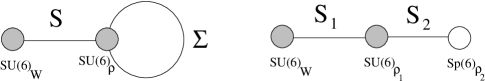
Figure 8: To extend $SU(6)/Sp(6)$ beyond the lightest $\rho$ to include the $a_{1}$ one must enlarge the gauge structure. To include the additional $a_{1}$, promote the gauged $Sp(6)_{\rho}$ to $SU(6)_{\rho}$, as depicted in the left figure. The following $\rho^{\prime}$ can be included by adding another $Sp(6)_{\rho}$, as shown in the right figure.

To model resonances beyond the $\rho$ in these non-QCD-like theories it is necessary to enlarge the gauge structure. To include the $a_{1}$ we promote the strongly gauged $Sp(6)_{\rho}$ to $SU(6)_{\rho}$ and include two non-linear sigma model fields: one a bi-fundamental under $SU(6)_{w}$ and $SU(6)_{\rho}$, $S$,and an anti-symmetric tensor under $SU(6)_{\rho}$, $\Sigma$. This action contains a single non-local operator:

$$\mathcal{L} = -\frac{1}{2}\mbox{Tr}\,P_{\mu\nu}^{2}+f^{2}\Big{(}\mbox{Tr}\,|DS|^{2}+c^{2}\mbox{Tr}\,|D\Sigma|^{2}+\kappa\mbox{Tr}\,|DS\Sigma|^{2}\Big{)}\,.$$ (3.25)

As in the case with only the $\rho$ incorporated, $\kappa$ alone determines the one-loop quadratically divergent counter-term for the effective potential. For $\kappa\neq 0$, there is a quadratic divergence, and we cannot reliably calculate the vacuum alignment using our techniques. For $\kappa=0$, the vector limit, the contribution to the effective potential from the $\rho$’s dominate over the contribution from the $a_{1}$, and we have the naive vacuum alignment. Thus, we need to introduce resonances beyond the $\rho$ and the $a_{1}$ if we wish to study possible modifications of vacuum alignment.

The next simplest theory includes the $\rho$, $a_{1}$ and the $\rho^{\prime}$. This theory has a strongly gauged $SU(6)_{\rho}$ and $Sp(6)_{\rho}$ and is depicted in Fig. 8. There are several non-local interactions. The Lagrangian is given by

$$\mathcal{L} = -\frac{1}{2}\mbox{Tr}\,W_{\mu\nu}^{2}-\frac{1}{2}\mbox{Tr}\,P_{\mu\nu}^{2}-\frac{1}{2}\rho_{\mu\nu}^{2}+f^{2}\Big{(}\mbox{Tr}\,|DS_{1}|^{2}+c^{2}\mbox{Tr}\,|DS_{2}|^{2}$$ (3.26)

$$\hskip 36.135pt+\kappa_{1}\mbox{Tr}\,|DS_{1}S_{2}|^{2}+\frac{\kappa_{2}}{4}\mbox{Tr}\,|DS_{2}\Sigma_{0}S_{2}^{T}|^{2}+\frac{\kappa^{\prime}}{4}\mbox{Tr}\,|DS_{1}S_{2}\Sigma_{0}S_{2}^{T}S_{1}^{T}|^{2}\Big{)}\,,$$

where we define $S_{j}=e^{i\,\pi_{j}/f}$.

3.3.1 Salvaging $SU(6)/Sp(6)$ Away from the Vector Limit?

In Sec. 3.2.2 we showed that the vector limit gave the wrong vacuum for the $SU(6)/Sp(6)$ to be a Little Higgs theory. However, the vector limit can be altered by mixing with heavier modes as we saw in Sec. 2.4. Given this, can we construct a theory incorporating higher modes, sufficiently far away from the single $\rho$ vector limit of Sec. 3.2.2, so that the theory has the vacuum required to be a Little Higgs model? At the same time, we wish to maintain a good description in terms of an effective Lagrangian of PNGB’s and light resonances without quadratic divergences in the Coleman-Weinberg potential. In the traditional sum rule picture, it is assumed that the vacuum is largely determined by the lowest resonances, which saturate spectral functions. We would like to understand the robustness of this result.

By modeling the $a_{1}$ resonances in the way we discussed here, it is possible to provide some more explicit understanding of how the vacuum could be modified from its naive alignment. Since the effective potential for the PNGB’s of the theory is produced by non-trivial mixing between spin-1 states after the inclusion of spontaneous and explicit symmetry breaking terms, it depends not only on the actual masses of the $a_{1}$ and $\rho$ fields, but also on the mixing with the low energy states. Most importantly, $a_{1}$’s and $\rho$’s contribute to such potential with opposite sign, so that it is in principle possible to reverse the naive sign of the Coleman-Weinberg potential by increasing the realtive importance of the $a_{1}$’s.

We performed extensive studies trying to reverse vacuum alignment, focusing in particular on cases in which only local operators are allowed at the effective Lagrangian level, in such a way as to soften, or even remove, UV cut-off dependences in the Coleman-Weinberg potential. We found that, indeed, thanks to the complicated form of mixing terms in the spin-1 field mass matrices, it appears possible to stabilize the vacuum, but only at the price of using negative values for the $\kappa$ factors, and somewhat large ratios between the gauge couplings. This implies that the vacuum can be stabilized only in the parameter space region where the theory starts to become strongly coupled: some of the states have masses close to the natural cut-off of the theory, and the validity of the effective field theory description becomes questionable. While not conclusive, this study does indicate that vacuum alignment seems to be more robust than what one might have naively expected.

4 Unitarity and Strong Coupling

Little Higgs models are non-renormalizable non-linear sigma models and so must become strongly coupled. At some scale, $\Lambda$, the low energy description of the theory becomes inadequate, and new physics (or strong coupling) sets in. Naive dimensional analysis (NDA) [16] gives a cut-off of $\Lambda\sim 4\pi f$. There are many simple refinements of the NDA estimate. One of the most common is the large $N_{c}$ refinement, which estimates $\Lambda\sim 4\pi f/N_{c}^{\frac{1}{2}}$. A similar result applies for a large number of fermions, $N_{f}$: $\Lambda\sim 4\pi/N_{f}^{\frac{1}{2}}$.

An alternate approach is to do a partial-wave unitarity analysis, as done for Little Higgs models in [25]. One examines the amplitudes of the Goldstone bosons scattering, and finds that the scattering becomes strong at

$$\Lambda_{U}\sim\sqrt{4\pi}f/\mathcal{N}^{\frac{1}{4}},$$ (4.1)

where $\mathcal{N}$ is the number of Goldstone bosons. $\mathcal{N}$ roughly scales as $N_{f}^{2}$, so this result for $\Lambda$ roughly matches the large $N_{f}$ refinement of NDA, up to a difference of $\sqrt{2\pi}$. In this large $N_{f}$ limit, the difference is due to conservatism – the partial wave analysis is more conservative than NDA. Note, chiral symmetry breaking cannot produce an arbitrarily large number of PNGBs for a fixed $N_{c}$: the number of PNGBs roughly scales as $\mathcal{N}\sim N_{f}^{2}$, and at sufficiently large $N_{f}$ the confining theory becomes asymptotically non-free.

Both the NDA and the partial wave analyses attempt to give an indication of where new physics modifies the scattering behavior of the Goldstone bosons. It is natural to inquire what form this new physics takes. There are some arguments that vector mesons are responsible for the unitarization of $\pi^{2}\rightarrow\pi^{2}$ scattering at intermediate energies, i.e. $\rho$ mesons soften the $\pi$ scattering. In this section we explore whether this possibility obtains. In fact, we find that incorporating the $\rho$ mesons does not result in a parametric rise in scale where perturbative unitarity is lost. There are special values of $\kappa$ where the leading $\pi^{4}$ interactions vanish but the $\xi^{2}\pi^{2}$ and $\xi^{4}$ interactions do not disappear.

While the $\rho$ does not provide a panacea, it can conceivably give a temporary postponement of the scale of perturbative unitarity violation. Recall that the coupling of the $\rho$ scales as $g_{\rho}\sim 4\pi/N_{c}^{\frac{1}{2}}$, so the mass of the $\rho$ scales as

$$m_{\rho}\sim\frac{4\pi f}{N_{c}^{\frac{1}{2}}}.$$ (4.2)

Note, this coincides with the large $N_{c}$ cut-off. In this large $N_{c}$ case, one might visualize a series of vector resonances, starting with the lowest $\rho$ states, serving to postpone unitarity violation. This is not dissimilar to the “Higgs”-less theories [26] or Randall-Sundrum I models that provide a window of unitarization mediated by Kaluza-Klein modes. For small $N_{c}$, where the vector resonances are heavy, it seems clear that the techni-$\rho$s are not responsible for unitarizing the scattering. In this case, incorporating a broad $\sigma$-like resonances seems more reasonable. We discuss this in more detail in Sec. 4.2. In this case, we interpret the partial wave unitarity scale as where the broad $\sigma$ resonance appears.

4.1 $\rho$’s and Unitarization

We now address the onset of strong coupling in the presence of the $\rho$’s. Therefore, we expect that the scale of strong pion scattering is modified by the addition of the $\rho$ mesons to the chiral Lagrangian. Unfortunately, the energy region where the $\rho$ is important for scattering is not in the equivalence region where $E\gg m_{\rho}$, meaning that the transverse components of the $\rho$ matter for scattering. This complicates the results. For simplicity we ignore this technicality and only consider the longitudinal component–our results will be most accurate in theories where the $\rho$’s are light.

To explore strong coupling, we first expand the original $\pi$ Lagrangian in Eq. 2.7 to quartic order in the fields to find how the interactions behave without the influence of the $\rho$:

$$\mathcal{L}_{\text{eff}}\supset\frac{2}{3f_{\pi}^{2}}\Gamma^{(4)}(\pi,D\pi)=\frac{2}{3f_{\pi}^{2}}\Gamma^{(4)}_{abcd}\pi^{a}\pi^{b}D\pi^{c}D\pi^{d},$$ (4.3)

where

$$\Gamma^{(4)}_{abcd}=\mbox{Tr}\,\tau_{a}\tau_{b}\tau_{c}\tau_{d}-\mbox{Tr}\,\tau_{a}\tau_{c}\tau_{b}\tau_{d}=\frac{1}{4}\Big{(}\delta_{ab}\delta_{cd}-\delta_{ac}\delta_{bd}\Big{)}.$$ (4.4)

Similarly, the chiral Lagrangian containing the $\rho$ can also be expanded to quartic order. One must take care to canonically normalize $\xi$, the longitudinal component of the $\rho$. In this case, the quartic interactions are

$$\mathcal{L} \supset \frac{2N_{\pi}^{2}}{3f_{\pi}^{2}}\Big{[}\Gamma^{(4)}\left((N_{\pi}^{-1}\pi+N_{\xi}^{-1}\xi),D(N_{\pi}^{-1}\pi+N_{\xi}^{-1}\xi)\right)$$ (4.5)

$$\hskip 28.90755pt+\Gamma^{(4)}\left((N_{\pi}^{-1}\pi-N_{\xi}^{-1}\xi),D(N_{\pi}^{-1}\pi-N_{\xi}^{-1}\xi)\right)$$

$$\hskip 28.90755pt+\frac{\kappa}{2}\Gamma^{(4)}(2N_{\pi}^{-1}\pi,2N_{\pi}^{-1}D\pi)\Big{]}.$$

This effective Lagrangian will break down due to strong coupling at energies not drastically different from $4\pi f_{\pi}$, even with the incorporation of the $\rho$’s into the Lagrangian.

In the vector limit the scattering simplifies significantly: the final term in the Lagrangian is absent and $N_{\pi}=N_{\xi}$. In the vector limit, the lowest scale of unitarity violation involves the scattering of the state

$$|\phi\rangle=\frac{1}{\sqrt{2}}(|\pi\rangle\pm|\xi\rangle).$$ (4.6)

This corresponds to a state localized in $\pi_{L}$ or $\pi_{R}$. This is clear from the geometric picture where the states with lowest scale of strong coupling are localized wave packets, rather than mass eigenstate. As localized object, they probe short distances, and thus the highest energies. As we move away from the vector limit, the most strongly coupled state is more $\pi$-like when $\kappa>0$ and more $\xi$-like when $\kappa<0$.

The scale of unitarity violation for a localized states is related to the $f$ of the adjacent link. As more modes are incorporated, the $f$ associated with each link increases relative to $f_{\pi}$:

$$f=n_{S}^{\frac{1}{2}}f_{\pi},$$ (4.7)

where $n_{S}$ is the number of sites. This increases the separation between $f_{\pi}$ and $f$, showing an improvement in the scattering behavior. The introduction of each vector resonance allows the temporary postponement of the scale of unitarity violation, similar to Higgsless theories of EWSB [26], where the new KK modes postpone the breakdown of unitarity in longitudinal $WW$ scattering.

In the generalized vector limit with $n_{S}$ sites, the scale of unitarity violation simply scales as

$$\Lambda_{U}\propto n_{S}^{\frac{1}{2}}f_{\pi}$$ (4.8)

because the $\Gamma^{(4)}$ tensors are block diagonal and different sets of pions don’t interact at leading order. On the other hand, if the theory is significantly away from the vector limit, the number of PNGBs in the final state increases as $n_{S}$, thus lowering the scale where unitarity violation would occur. The scale of unitarity violation scales as

$$\Lambda_{U}\propto n_{S}^{\frac{1}{4}}f_{\pi}.$$ (4.9)

Thus the vector limit appears to help stave off unitarity violation making the theory healthy over a larger energy regime.

4.2 The $\sigma$ Resonance

There are several broad light isospin singlet scalar resonances in QCD, typically called $f_{0}$ resonances. The first $f_{0}$ lies in the 500 MeV range with a width roughly as big as its mass. These states are capable of unitarizing $\pi\pi$ scattering exactly as the Higgs boson does – by being the fluctuation of the vacuum expectation value.

In QCD $N_{c}$ and $N_{f}$ are the same, and the $\rho$ and $f_{0}$ are roughly degenerate. In this section we argue that in the limit where there are a large number of pions (corresponding to a large $N_{f}$), the $f_{0}$ resonance becomes light and is responsible for unitarizing the Nambu-Goldstone boson scattering. Typically several scalar resonances are necessary to completely unitarize $\pi\pi$ scattering up to high energies. We will explore the quantum numbers of these resonances.

We now consider the scattering of the Goldstone bosons in the Littlest Higgs ($SU(5)/SO(5)$) model in some detail, and show the role a $\sigma$ resonance could play in unitarizing the theory. Here we discuss the $\sigma$’s in the theory that does not incorporate the techni-$\rho$s; it is possible to extend this analysis to theories that model these states.

It is useful to decompose the $\pi\pi$ scattering amplitude into representations of the unbroken symmetry group. In the Littlest Higgs model the $\pi\pi\rightarrow\pi\pi$ scattering can be decomposed into various $SO(5)$ channels:

$$\mathbf{14}\otimes\mathbf{14}\rightarrow\mathbf{1}\oplus\mathbf{10}\oplus\mathbf{14}\oplus\cdots\,.$$ (4.10)

Each of the partial wave amplitudes has a different scale of unitarity violation. It is the fluctuation in the singlet channel (the direction of the vev) that has the lowest scale of unitarity violation. This is because the other channels have smaller Clebsch-Gordon coefficients in the decomposition. A single, broad scalar should be expected for the lightest $\sigma$ resonance, unitarizing this singlet channel. Other representations are important for staving off unitarity violation in the other channels.

We can find the relevant $\sigma$ model by considering a linear $\sigma$ model for the breaking of $SU(5)\rightarrow SO(5)$. To accomplish this breaking, a symmetric tensor of $SU(5)$ acquires a vev. The symmetric tensor decomposes under $SO(5)$ as:

$$30\rightarrow\mathbf{14}^{-}\oplus\mathbf{14}^{+}\oplus\mathbf{1}^{+}\oplus\mathbf{1}^{-}.$$ (4.11)

We have introduced a “charge conjugation” $\mathbb{Z}_{2}$ symmetry under which the $\rho$’s are even, but the $a_{1}$ is odd. The $\mathbf{1}^{+}$ is the state responsible for unitarizing the most strongly coupled singlet channel. The $\mathbf{14}^{-}$ are the pions of the Little Higgs theory. As $N_{f}$ grows large, we believe that the $\sigma$ becomes light and is responsible for unitarity violation. This is very closely related the restoration of chiral symmetry at large $N_{f}$ where one still has confinement but no chiral symmetry breaking. A possible theory for the linear sigma model that displays this behavior is:

$$\mathcal{L}_{\text{eff}}\sim|\partial\Phi|^{2}-V(\Phi),\hskip 36.135ptV(\Phi)=\lambda(N_{f_{c}}-N_{f})(|\Phi|^{2}-f^{2})^{2}.$$ (4.12)

As $N_{f}$ approaches $N_{f_{c}}$ the $\sigma$ resonance becomes light, after $N_{f_{c}}$ chiral symmetry is restored. The dynamics is a continuous in $N_{f}$, and as $N_{f}$ approaches the critical number of flavors to restore chiral symmetry the $\sigma$ resonances become light and degenerate with the $\pi$, filling out an entire chiral multiplet. Therefore, in the large $N_{f}$ limit, the scale of unitarity violation seems closely tied to the presence of additional strongly coupled, broad scalar resonances rather than new vector mesons. New vector resonances could cut-off gauge quadratic divergences. If they are mandated to be light to unitarize the theory, then quadratic divergences may be cut-off well beneath the NDA scale. On the other hand, if the $\sigma$ is unitarizing the theory, the vector resonances can be heavy, and the divergences will be cut-off closer to the NDA scale.

4.3 Unitarity Moral

Regardless of whether we place our faith in the NDA analysis or, alternately, the partial wave unitarity analysis, it is clear that new modes are expected to appear beneath $4\pi f$.

In the previous sections we illustrated the effect of the introduction of $\rho$-type resonances, showing that they can soften the cut-off dependence of the theory, thus making previously incalculable quantities calculable. In this section we analyzed the role of these $\rho$’s in unitarizing $\pi-\pi$ scattering amplitude, as compared to that of $\sigma$-type states.

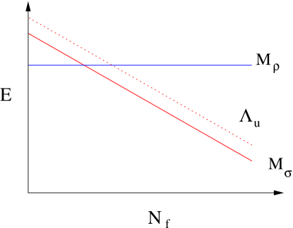
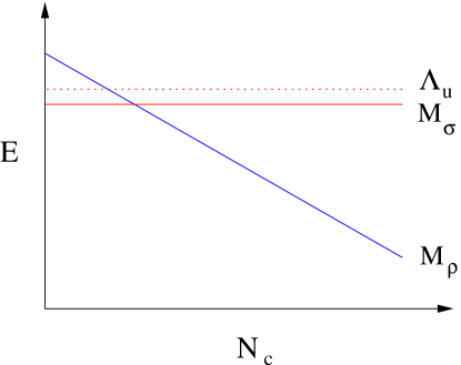
Figure 9: The left figure illustrates how the mass of the lightest $\sigma$ and $\rho$ and scale of unitarity violation in $\pi\pi$ scattering scale with $N_{f}$. The $\sigma$ resonances become light and unitarize the scattering in a Higgs-like manner. The right figure show how they vary with $N_{c}$. The $\rho$ resonances become light (and simultaneously weakly interacting) in the large $N_{c}$ limit and can stave off unitarity violation as in Randall-Sundrum models or Higgsless models.

Our results are well illustrated by Fig 9. It is clear that, as suggested by the intuition, the scale of unitarization is strongly correlated with the mass of the $\sigma$ fields. A partial unitarization can be achieved with the introduction of a tower of vector resonances. If these resonances are present, the Goldstone boson scattering may remain well-behaved up to higher energies, even without the introduction of a $\sigma$ resonance. For the vector resonances to be important for unitarizing scattering, they should light; however, from discussion about little Higgs models, this possibility seems phenomenologically disastrous: they contribute to a light Higgs and a large $S$ parameter. Thus we expect broad $\sigma$ resonances for these models to unitarize the scattering if Little Higgs models are to be phenomenologically viable. So while $\sigma$ resonances might be crucial for understanding unitarity, they are essentially invisible and do not affect the low energy phenomenology.

5 Conclusions

Using effective field theory techniques, we have studied vector resonances, moderately light relative to the scale of strong dynamics. This approach allows the exploration of the vector limit, a point of enhanced symmetry. Georgi’s vector limit corresponds to a theory that is local in its theory space description. In the vector limit, the lightest $\rho$ regulates the leading cut-off sensitive operators in the chiral Lagrangian. In QCD, this corresponds to a softening of the divergence in the $\pi^{\pm}-\pi^{0}$ mass difference.

It is not clear that Georgi’s vector limit is in any way fundamental, and whether we expect it to hold in a generic (non-QCD) theory of strong coupling. However, if it does apply, then it can have important phenomenological consequences. We considered these implications by extrapolating this approach to the structure of techni-$\rho$s in Little Higgs theories. By including techni-$\rho$s in these theories and assuming the analogue of the vector limit, we were able to discuss previously ultraviolet sensitive, phenomenologically relevant quantities. For example, by using large $N_{c}$ arguments, we argued that the mass of the Higgs boson in the Littlest Higgs theory is roughly the mass of $m_{W}$ and decreases as the techni-$\rho$s become light. It should be noted that there are large radiative corrections from the top quark that we did not estimate.

Finally, we briefly explored unitarity violation in Little Higgs models. We argued that the scale of unitarity break-down likely points to broad $\sigma$-like resonances. If, instead of $\sigma$-like fields, this scale pointed to the presence of techni-$\rho$’s, then gauge quadratic divergences would be cut off at this scale. The result would be a too-light Higgs boson.

We close with a few directions for further work. In principle, the techni-$\rho$ vector resonances can have masses similar to those of the additional gauge bosons of Little Higgs models. This could change the collider phenomenology predictions, and conceivably modify precision electroweak predictions. Using the formalism introduced here, it should be possible to pursue this question further. Also, there is a UV completion for the Littlest Higgs that uses a strongly coupled supersymmetric $SO(7)$ gauge theory [27]. Using the ideas in this note detailed predictions of the semi-perturbative regime could be analyzed.

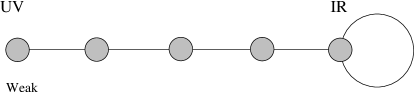
Figure 10: A schematic depiction of how the techni-$\rho$ resonances turn into deconstructed space maps into a holographic extra dimension. The weakly gauged group is on the left. The additional sites represent strongly gauged techni-$\rho$s. In the IR, chiral symmetry is broken by a non-linear sigma model field.

These ideas of modeling the the techni-$\rho$ resonances are closely related to deconstructing AdS [28, 29]. As the number of sites grows large, theory space reconstructs an extra-dimension as in Fig 10. It would be interesting to explore this structure to see if deconstructing AdS leads to some insight into the generalized vector limit.

References

- [1] H. Georgi and A. Pais, Phys. Rev. D 12, 508 (1975). D. B. Kaplan and H. Georgi, Phys. Lett. B 136, 183 (1984). D. B. Kaplan, H. Georgi and S. Dimopoulos, Phys. Lett. B 136, 187 (1984). H. Georgi, D. B. Kaplan and P. Galison, Phys. Lett. B 143, 152 (1984). H. Georgi and D. B. Kaplan, Phys. Lett. B 145, 216 (1984). M. J. Dugan, H. Georgi and D. B. Kaplan, Nucl. Phys. B 254, 299 (1985).
- [2] N. Arkani-Hamed, A. G. Cohen and H. Georgi, Phys. Lett. B 513, 232 (2001), [arXiv:hep-ph/0105239]. N. Arkani-Hamed, A. G. Cohen, T. Gregoire and J. G. Wacker, JHEP 0208, 020 (2002) [arXiv:hep-ph/0202089]. N. Arkani-Hamed, A. G. Cohen, E. Katz, A. E. Nelson, T. Gregoire and J. G. Wacker, JHEP 0208, 021 (2002) [arXiv:hep-ph/0206020]. T. Gregoire and J. G. Wacker, JHEP 0208, 019 (2002) [arXiv:hep-ph/0206023]. D. E. Kaplan and M. Schmaltz, JHEP 0310, 039 (2003) [arXiv:hep-ph/0302049]. J. G. Wacker, arXiv:hep-ph/0208235; W. Skiba and J. Terning, Phys. Rev. D 68, 075001 (2003) [arXiv:hep-ph/0305302]. S. Chang, JHEP 0312, 057 (2003) [arXiv:hep-ph/0306034]; M. Schmaltz, Nucl. Phys. Proc. Suppl. 117, 40 (2003) [arXiv:hep-ph/0210415]; H. C. Cheng and I. Low, JHEP 0309, 051 (2003) [arXiv:hep-ph/0308199].
- [3] N. Arkani-Hamed, A. G. Cohen, E. Katz and A. E. Nelson, JHEP 0207, 034 (2002)
- [4] I. Low, W. Skiba and D. Smith, Phys. Rev. D 66, 072001 (2002) [arXiv:hep-ph/0207243].
- [5] M. Bando, T. Kugo, S. Uehara, K. Yamawaki and T. Yanagida, Phys. Rev. Lett. 54, 1215 (1985). M. Bando, T. Fujiwara and K. Yamawaki, Prog. Theor. Phys. 79, 1140 (1988). M. Bando, T. Kugo and K. Yamawaki, Phys. Rept. 164, 217 (1988).
- [6] H. Georgi, Nucl. Phys. B 331, 311 (1990).
- [7] N. Arkani-Hamed, A. G. Cohen and H. Georgi, Phys. Rev. Lett. 86, 4757 (2001) [arXiv:hep-th/0104005]; C. T. Hill, S. Pokorski and J. Wang, Phys. Rev. D 64, 105005 (2001) [arXiv:hep-th/0104035].
- [8] M. Harada, M. Tanabashi and K. Yamawaki, Phys. Lett. B 568, 103 (2003) [arXiv:hep-ph/0303193].
- [9] N. Arkani-Hamed, H. Georgi and M. D. Schwartz, Annals Phys. 305, 96 (2003) [arXiv:hep-th/0210184].
- [10] D. T. Son and M. A. Stephanov, Phys. Rev. D 69, 065020 (2004) [arXiv:hep-ph/0304182].
- [11] K. Kawarabayashi and M. Suzuki, Phys. Rev. Lett. 16, 255 (1966). Riazuddin and Fayyazuddin, Phys. Rev. 147, 1071 (1966).
- [12] S. R. Coleman and E. Weinberg, Phys. Rev. D 7, 1888 (1973).
- [13] T. Das, G. S. Guralnik, V. S. Mathur, F. E. Low and J. E. Young, Phys. Rev. Lett. 18, 759 (1967); I. Bars, M. B. Halpern and K. D. Lane, Nucl. Phys. B 65, 518 (1973); S. Chadha and M. E. Peskin, Nucl. Phys. B 187, 541 (1981); S. Chadha and M. E. Peskin, Nucl. Phys. B 185, 61 (1981).
- [14] R. S. Chivukula, M. Kurachi and M. Tanabashi, arXiv:hep-ph/0403112.
- [15] T. Gregoire and J. G. Wacker, arXiv:hep-ph/0207164. N. Arkani-Hamed, A. G. Cohen, D. B. Kaplan, A. Karch and L. Motl, JHEP 0301, 083 (2003) [arXiv:hep-th/0110146]; A. Iqbal and V. S. Kaplunovsky, JHEP 0405, 013 (2004) [arXiv:hep-th/0212098].
- [16] A. Manohar and H. Georgi, Nucl. Phys. B 234, 189 (1984); H. Georgi and L. Randall, Nucl. Phys. B 276, 241 (1986).
- [17] G. ’t Hooft, Nucl. Phys. B 72, 461 (1974).
- [18] R. F. Dashen, Phys. Rev. 183, 1245 (1969). S. Weinberg, Phys. Rev. D 13, 974 (1976). S. Weinberg, Phys. Rev. D 19 (1979) 1277.
- [19] M. E. Peskin, Nucl. Phys. B 175, 197 (1980); J. Preskill, Nucl. Phys. B 177, 21 (1981); M. E. Peskin, SLAC-PUB-3021 Lectures presented at the Summer School on Recent Developments in Quantum Field Theory and Statistical Mechanics, Les Houches, France, Aug 2 - Sep 10, 1982.
- [20] S. Weinberg, Phys. Rev. Lett. 18, 507 (1967); C. W. Bernard, A. Duncan, J. LoSecco and S. Weinberg, Phys. Rev. D 12, 792 (1975).
- [21] J. L. Hewett, F. J. Petriello and T. G. Rizzo, JHEP 0310, 062 (2003) [arXiv:hep-ph/0211218]. C. Csaki, J. Hubisz, G. D. Kribs, P. Meade and J. Terning, Phys. Rev. D 67, 115002 (2003) [arXiv:hep-ph/0211124]. W. Kilian and J. Reuter, arXiv:hep-ph/0311095.
- [22] G. Burdman, M. Perelstein and A. Pierce, Phys. Rev. Lett. 90, 241802 (2003) [Erratum-ibid. 92, 049903 (2004)] [arXiv:hep-ph/0212228]. T. Han, H. E. Logan, B. McElrath and L. T. Wang, Phys. Rev. D 67, 095004 (2003) [arXiv:hep-ph/0301040]. M. Perelstein, M. E. Peskin and A. Pierce, Phys. Rev. D 69, 075002 (2004) [arXiv:hep-ph/0310039].
- [23] S. Chang and J. G. Wacker, Phys. Rev. D 69, 035002 (2004) [arXiv:hep-ph/0303001].
- [24] T. Gregoire, D. R. Smith and J. G. Wacker, arXiv:hep-ph/0305275. C. Csaki, J. Hubisz, G. D. Kribs, P. Meade and J. Terning, Phys. Rev. D 68, 035009 (2003) [arXiv:hep-ph/0303236].
- [25] S. Chang and H. J. He, arXiv:hep-ph/0311177.
- [26] C. Csaki, C. Grojean, H. Murayama, L. Pilo and J. Terning, arXiv:hep-ph/0305237. C. Csaki, C. Grojean, L. Pilo and J. Terning, arXiv:hep-ph/0308038. Y. Nomura, JHEP 0311, 050 (2003) [arXiv:hep-ph/0309189]. R. Barbieri, A. Pomarol and R. Rattazzi, arXiv:hep-ph/0310285.
- [27] A. E. Nelson, arXiv:hep-ph/0304036. E. Katz, J. y. Lee, A. E. Nelson and D. G. E. Walker, arXiv:hep-ph/0312287.
- [28] J. M. Maldacena, Adv. Theor. Math. Phys. 2, 231 (1998) [Int. J. Theor. Phys. 38, 1113 (1999)] [arXiv:hep-th/9711200]. L. Randall and R. Sundrum, Phys. Rev. Lett. 83, 3370 (1999) [arXiv:hep-ph/9905221].
- [29] H. C. Cheng, C. T. Hill and J. Wang, Phys. Rev. D 64, 095003 (2001) [arXiv:hep-ph/0105323]. H. Abe, T. Kobayashi, N. Maru and K. Yoshioka, Phys. Rev. D 67, 045019 (2003) [arXiv:hep-ph/0205344]. A. Falkowski and H. D. Kim, JHEP 0208, 52 (2002) [arXiv:hep-ph/0208058]. L. Randall, Y. Shadmi and N. Weiner, JHEP 0301, 055 (2003) [arXiv:hep-th/0208120].