1 CP Violation in the Standard Model

In the standard model (SM), CP violation is due to a complex phase in the Cabibbo-Kobayashi-Maskawa (CKM) quark mixing matrix [1]. A convenient approximate parametrization, due to Wolfenstein [2], follows from the (experimental) fact that one can write the elements of the CKM matrix in terms of powers of the Cabibbo angle, $\lambda=0.22$:

$$\left(\begin{array}[]{ccc}1-\frac{1}{2}\lambda^{2}&\lambda&A\lambda^{3}\left(\rho-i\eta\right)\\ -\lambda&1-\frac{1}{2}\lambda^{2}&A\lambda^{2}\\ A\lambda^{3}\left(1-\rho-i\eta\right)&-A\lambda^{2}&1\end{array}\right).$$ (1)

It is the appearance of the term $i\eta$ which is responsible for CP violation. To O($\lambda^{3}$), this term appears only in $V_{ub}$ and $V_{td}$.

Writing the corner elements as $V_{ub}\equiv|V_{ub}|e^{-i\gamma}$ and $V_{td}\equiv|V_{td}|e^{-i\beta}$, and using the unitarity of the CKM matrix, $V_{ud}V^{*}_{ub}+V_{cd}V^{*}_{cb}+V_{td}V^{*}_{tb}=0$, the CKM phase information can be elegantly described by the so-called unitarity triangle (Fig. 1) [1]. The interior angles, $\alpha$, $\beta$ and $\gamma$ describe CP violation in $B$ decays. In order to test the SM explanation of CP violation, the idea is to measure the angles and sides of the unitarity triangle in as many ways as possible, and to look for consistency. A discrepancy points to the presence of physics beyond the SM.

Figure 1: The unitarity triangle.

2 CP Violation in the $B$ System

In general, CP violation requires the interference of two amplitudes. Consider the decay $B\to f$ and suppose that there are two amplitudes, with different weak (CP-odd) and strong (CP-even) phases. The strong phases are typically due to QCD processes, which are insensitive to whether quarks or antiquarks are involved. I will return in Sec. 4 to the issue of strong phases. The amplitude for the CP-conjugate process ${\bar{B}}\to{\bar{f}}$ is obtained by simply reversing the signs of the weak phases. We have

$$A(B\to f) = A_{1}e^{i\phi_{1}}e^{i\delta_{1}}+A_{2}e^{i\phi_{2}}e^{i\delta_{2}}~{},$$

$$A({\bar{B}}\to{\bar{f}}) = A_{1}e^{-i\phi_{1}}e^{i\delta_{1}}+A_{2}e^{-i\phi_{2}}e^{i\delta_{2}}~{},$$ (2)

where $\phi_{1,2}$ and $\delta_{1,2}$ represent the weak and strong phases, respectively.

If CP is violated, matter and antimatter behave differently. Thus, CP violation is signalled by a difference in the rates for the process and antiprocess. We can therefore define the direct CP asymmetry

$$A_{f}^{dir}\equiv\frac{\Gamma(B\to f)-\Gamma({\bar{B}}\to{\bar{f}})}{\Gamma(B\to f)+\Gamma({\bar{B}}\to{\bar{f}})}=-\frac{2A_{1}A_{2}\sin\Phi\sin\Delta}{A_{1}^{2}+A_{2}^{2}+2A_{1}A_{2}\cos\Phi\cos\Delta}~{},$$ (3)

where $\Phi\equiv\phi_{1}-\phi_{2}$ and $\Delta\equiv\delta_{1}-\delta_{2}$. Experimentally, one measures a direct CP asymmetry by simply comparing the rates for the two processes. Any difference reflects CP violation. However, recall that the aim is to extract CKM parameters. From the above expression, we see that the direct CP asymmetry $A_{f}^{dir}$ depends on the (unknown) strong phase difference $\Delta$. Thus, one cannot extract the weak phase information $\Phi$ without hadronic input.

Fortunately, there is another measure of CP violation, which relies on $B^{0}$–${\bar{B}}^{0}$ mixing. If one chooses a final state $f$ to which both $B^{0}$ and ${\bar{B}}^{0}$ can decay, then the amplitudes $B^{0}\to f$ and $B^{0}\to{\bar{B}}^{0}\to f$ will interfere, leading to CP violation.

In order for this mechanism to produce sizeable effects, large $B^{0}$–${\bar{B}}^{0}$ mixing is required. Fortunately, in 1987 it was found that large mixing is present [3]. This is arguably the most important discovery in particle physics in the last 20 years.

The size of this mixing was a great surprise. While it is known that $\Delta M_{d}\sim m_{t}^{2}$, in 1987 it was expected that $m_{t}\sim 10$ GeV, which would lead to small mixing. Few people considered the possibility of large $m_{t}$. One exception is Ref. [4], by B. A. Campbell and P. J. O’Donnell. In this paper, various $B$ processes were considered, including mixing, for values $m_{t}/M_{W}\leq 3.5$. (Experimentally, it is found that $m_{t}/M_{W}\sim 2$.) Thus, these authors actually anticipated the large mixing result.

In the presence of large $B^{0}$–${\bar{B}}^{0}$ mixing, one can measure an indirect CP asymmetry. There are many final states $f$ which can be used. The simplest case, which is described below, is where $f$ is a CP eigenstate. Because of mixing, a particle which is “born” as a $B^{0}$ will quantum-mechanically evolve in time into $B^{0}(t)$, a mixture of $B^{0}$ and ${\bar{B}}^{0}$. The measurement of the time-dependent decay rate then yields two measures of CP violation, $a_{dir}$ and $a_{indir}$:

$$\Gamma(B^{0}(t)\to f)\sim B+a_{dir}\cos(\Delta Mt)+a_{indir}\sin(\Delta Mt)~{},$$ (4)

with

$$B\equiv\frac{1}{2}\left(|A|^{2}+|{\bar{A}}|^{2}\right)~{},~{}a_{dir}\equiv\frac{1}{2}\left(|A|^{2}-|{\bar{A}}|^{2}\right)~{},~{}a_{indir}\equiv{\rm Im}\left(e^{-2i\phi_{\scriptscriptstyle M}}{A}^{*}{\bar{A}}\right)~{},$$ (5)

where $\phi_{\scriptscriptstyle M}$ is the phase of $B^{0}$–${\bar{B}}^{0}$ mixing. The quantity $a_{dir}$ is related to the direct CP asymmetry [Eq. (3)]. On the other hand, the indirect CP asymmetry $a_{indir}$ arises due to $B^{0}$–${\bar{B}}^{0}$ mixing. The key point here, which will be used later, is that the measurement of $\Gamma(B^{0}(t)\to f)$ yields 3 observables.

Note that if there is only a single decay amplitude in $B^{0}\to f$, i.e. $A_{2}=0$ in Eq. (2), then $a_{dir}=0$. However, we still have $a_{indir}\neq 0$. In fact, this is the most interesting scenario, since in this case all dependence on the unknown strong phases vanishes in $a_{indir}$.

Ideally, each of $\alpha$, $\beta$ and $\gamma$ could be measured in this way. However, although many techniques have been proposed for getting at the CP phases, only $\beta$ can be measured cleanly through $a_{indir}$. Here one uses the decay $B_{d}^{0}(t)\to J/\psi K_{\scriptscriptstyle S}$, dominated (to a very good approximation) by the ${\bar{b}}\to{\bar{c}}c{\bar{s}}$ tree amplitude, which is proportional to $V_{cb}^{*}V_{cs}$ and is real. In this case the direct CP asymmetry vanishes, and indirect CP violation then probes the phase of $B_{d}^{0}$–${\overline{B_{d}^{0}}}$ mixing: $2~{}{\rm arg}(V_{tb}^{*}V_{td})=-2\beta$.

Both BaBar and Belle have measured this CP phase, with the world average being [5]

$$\sin 2\beta=0.736\pm 0.049~{}.$$ (6)

As we will see, this agrees with independent measurements.

The phase $\alpha$ can be extracted from $B_{d}^{0}(t)\to\pi^{+}\pi^{-}$. Here the decay has two contributions (see Fig. 2). The tree diagram ($A_{1}$) is proportional to $V_{ub}^{*}V_{ud}$. The penguin contribution has pieces proportional to $V_{ub}^{*}V_{ud}$, $V_{cb}^{*}V_{cd}$ and $V_{tb}^{*}V_{td}$. CKM unitarity can be used to write the $V_{cb}^{*}V_{cd}$ piece in terms of the other two. The tree amplitude can then be redefined to include the penguin contribution proportional to $V_{ub}^{*}V_{ud}$. The penguin amplitude ($A_{2}$) can therefore be taken to be $\sim V_{tb}^{*}V_{td}$. If the penguin contribution were zero, the indirect CP asymmetry would probe $2~{}{\rm arg}(V_{tb}^{*}V_{td}V_{ub}V_{ud}^{*})=-2(\beta+\gamma)\sim 2\alpha$. Unfortunately, $A_{2}\neq 0$, i.e. the penguins are non-negligible. Thus, $a_{indir}$ does not probe $\alpha$ cleanly.

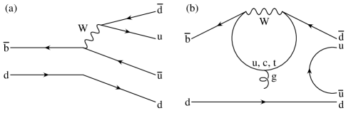
Figure 2: The tree and penguin amplitudes contributing to $B_{d}^{0}\to\pi^{+}\pi^{-}$.

Fortunately, a method has been constructed for removing the “penguin pollution” [6]. The point is that $B_{d}^{0}\to\pi^{+}\pi^{-}$ is related by isospin to $B^{+}\to\pi^{+}\pi^{0}$ and $B_{d}^{0}\to\pi^{0}\pi^{0}$. Using isospin, the measurement of the branching ratios for $B^{+}\to\pi^{+}\pi^{0}$ and $B_{d}^{0}\to\pi^{0}\pi^{0}$ (and their CP-conjugate decays) allows us to remove the penguin pollution from $\Gamma(B_{d}^{0}(t)\to\pi^{+}\pi^{-})$, and obtain $\alpha$ cleanly.

At present, Belle and BaBar have made all of the above measurements except for the individual $B^{0}\to\pi^{0}\pi^{0}$ and ${\bar{B}}^{0}\to\pi^{0}\pi^{0}$ rates. It is not clear exactly when these will be made, but it is possible that a full isospin analysis will be done, and $\alpha$ extracted, by the summer of 2005.

For obtaining the angle $\gamma$, many methods have been proposed. Some of these, such as $B\to DK$ [7] have little theoretical error; others require theoretical input. I will describe one of the second class of methods. There are two reasons for this. First, I will come back to this type of technique when discussing the measurement of new-physics parameters. Second, and more importantly, this method is being used by BaBar to extract $\gamma$.

Consider the decay $B_{d}^{0}(t)\to D^{(*)+}D^{(*)-}$ [8]. This is a ${\bar{b}}\to{\bar{c}}c{\bar{d}}$ transition and has penguin pollution (see Fig. 3). The tree amplitude is $\sim V_{cb}^{*}V_{cd}$ and is real. The penguin amplitude can be taken to be $\sim V_{ub}^{*}V_{ud}$ after CKM unitarity is applied and the tree redefined (as in $B_{d}^{0}\to\pi^{+}\pi^{-}$). The $B_{d}^{0}\to D^{(*)+}D^{(*)-}$ amplitude can then be written as

$$A\sim Te^{i\delta_{T}}+Pe^{i\gamma}e^{i\delta_{P}}~{},$$ (7)

in which we have explictly written the weak phase $\gamma$ and the strong phases $\delta_{T,P}$.

Figure 3: The tree and penguin amplitudes contributing to $B_{d}^{0}\to D^{+}D^{-}$.

It is straightforward to count the number of theoretical parameters. There are 4: $T$, $P$, $\gamma$ and ${\delta}\equiv{\delta}_{T}-{\delta}_{P}$. (The phase of $B_{d}^{0}$-${\overline{B_{d}^{0}}}$ mixing, $\beta$, is assumed to be measured in $B_{d}^{0}(t)\to J/\psi K_{\scriptscriptstyle S}$.) However, as noted earlier, the measurement of $B_{d}^{0}(t)\to D^{+}D^{-}$ yields only 3 observables. Thus, in order to extract $\gamma$, it is necessary to add some theoretical input.

This comes from $B_{d}^{0}\to D_{s}^{(*)+}D^{(*)-}$, which is a ${\bar{b}}\to{\bar{c}}c{\bar{s}}$ decay. It also receives both a tree and penguin contribution (see Fig. 4):

$$A^{D_{s}}=T^{\prime}\,V_{cb}^{*}V_{cs}+P^{\prime}\,V_{ub}^{*}V_{us}\approx T^{\prime}e^{i\delta^{\prime}_{T}}~{}.$$ (8)

Here the last approximate equality arises from the fact that $\left|{V_{ub}^{*}V_{us}/V_{cb}^{*}V_{cs}}\right|\simeq 2\%$. Thus, the decay $B_{d}^{0}\to D_{s}^{(*)+}D^{(*)-}$ is dominated by the tree contribution, and the measurement of its rate yields $T^{\prime}$.

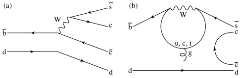
Figure 4: The tree and penguin amplitudes contributing to $B_{d}^{0}\to D_{s}^{+}D^{-}$.

We now make the flavour SU(3) assumption that

$$\frac{\lambda T^{\prime}}{T}=1~{}.$$ (9)

Given the knowledge of $T^{\prime}$, this assumption gives us $T$. Eq. (7) then contains only 3 theoretical unknowns, and the 3 experimental measurements in $B_{d}^{0}(t)\to D^{(*)+}D^{(*)-}$ can be used to obtain $\gamma$.

The main theoretical error in this method is the SU(3)-breaking effect in Eq. (9. The leading-order error is simply given by the ratio of decay constants, which has been calculated on the lattice with good precision: $f_{D_{s}}/f_{D}=1.22\pm 0.04$ [9]. The remaining error is due to second-order effects and is estimated to be $\sim 10\%$.

As noted above, this method is being used by BaBar to get $\gamma$. It is possible that we will have a first measurement of $\gamma$ this summer (2004).

3 New Physics Signals

Above, I have described some of the methods used to obtain CKM phase information. Any discrepancy in the SM description of CP violation points to the presence of physics beyond the standard model. There are in fact many signals of such new physics (NP). I list several of these below.

One test is to compare two $B$ decay modes which in the SM measure the same CP phase. For example, we know that $\beta$ is obtained in $B_{d}^{0}(t)\to J/\psi K_{\scriptscriptstyle S}$. But $\beta$ can also be extracted, with little theoretical error, from pure ${\bar{b}}\to{\bar{s}}$ penguin decays such as $B_{d}^{0}(t)\to\phi K_{\scriptscriptstyle S}$.

The latest data on measurements of $\sin 2\beta$ as extracted from $B$ charmonium decays and ${\bar{b}}\to{\bar{s}}$ penguin decays are shown in Fig. 5 [5]. Although the BaBar measurement of $\sin 2\beta$ in $B_{d}^{0}(t)\to\phi K_{\scriptscriptstyle S}$ agrees with that from $B_{d}^{0}(t)\to J/\psi K_{\scriptscriptstyle S}$ (within errors), Belle finds that $\sin 2\beta=-1$, in clear disagreement with Eq. (6). In fact, the value of $\sin 2\beta$ extracted from all ${\bar{b}}\to{\bar{s}}$ penguin decays is $3.1\sigma$ below that from charmonium decays. Although not yet statistically significant, this may be pointing to NP.

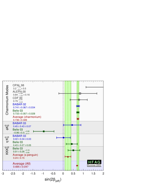
Figure 5: The latest data on the extraction of $\sin 2\beta$ from measurements of CP violation in $B\to$ charmonium decays and in ${\bar{b}}\to{\bar{s}}$ penguin decays.

As noted above, there are in fact many ways to measure CP phases, often with some theoretical input [10]. If the values of the CP angles in these modes disagree with one another at a level beyond the theoretical error, this implies new physics.

Another hint of new physics comes from $B\to K\pi$ decays. It is possible to write the amplitudes for these decays in terms of diagrams ($T$, $P$, etc.) [11]. Some diagrams are expected to be negligible (e.g. exchange- and annihilation-type amplitudes), in which case we have $R_{c}=R_{n}$ [12], where

$$R_{c}\equiv\frac{2{\bar{\Gamma}}(B^{+}\to K^{+}\pi^{0})}{{\bar{\Gamma}}(B^{+}\to K^{0}\pi^{+})}~{}~{},~{}~{}~{}~{}R_{n}\equiv\frac{{\bar{\Gamma}}(B_{d}^{0}\to K^{+}\pi^{-})}{2{\bar{\Gamma}}(B_{d}^{0}\to K^{0}\pi^{0})}~{}.$$ (10)

However, present data yields [5]

$$R_{c}=1.42\pm 0.18~{}~{},~{}~{}~{}~{}R_{n}=0.89\pm 0.13~{}.$$ (11)

There is a discrepancy of $2.4\sigma$ between $R_{c}$ and $R_{n}$, perhaps suggesting the presence of NP.

There are several observables which are zero (or small) in the SM. For example, the phase of $B_{s}^{0}$–${\overline{B_{s}^{0}}}$ mixing is $2~{}{\rm arg}(V_{tb}^{*}V_{ts})\simeq 0$. This phase can be measured via the CP asymmetry in $B_{s}^{0}(t)\to J/\psi\eta$. If this mixing phase is found to be large, this would indicate NP.

As another example, $BR(B\to\ell^{+}\ell^{-})\sim m_{\ell}^{2}/M_{B}^{2}$. That is, this decay is helicity-suppressed, and so its branching ratio is expected to be tiny. (An exception is $BR(B_{s}^{0}\to\tau^{+}\tau^{-})\sim 10^{-6}$.) These rates were first estimated by B. A. Campbell and P. J. O’Donnell in Ref. [4]. If, for example, $B_{s}^{0}\to\mu^{+}\mu^{-}$ is seen at a measurable level, NP must be present (e.g. SUSY models with large $\tan\beta$).

Since $b\to s\gamma$ is dominated by a single amplitude in the SM, it is expected that the inclusive $A_{CP}^{dir}(b\to s\gamma)\simeq 0$ [13]. This is another good area to search for new physics. (As an aside, Pat O’Donnell is probably best known for his calculation of $b\to s\gamma$ in the SM, see Ref. [14]. These references also discuss other rare decays, such as $B\to s\ell^{+}\ell^{-}$.)

Another interesting area of study is $B\to V_{1}V_{2}$ decays, where $V_{1}$ and $V_{2}$ are vector mesons. It is possible to measure the CP-violating triple-product correlation (TP) ${\vec{\varepsilon}}_{1}^{*\scriptscriptstyle T}\times{\vec{\varepsilon}}_{2}^{*\scriptscriptstyle T}\cdot{\hat{p}}$, where ${\vec{\varepsilon}}_{1,2}^{*\scriptscriptstyle T}$ are the polarizations of the vector mesons and ${\hat{p}}$ is the final-state momentum. In the SM, all TP’s are expected to vanish or be very small, making them an excellent place to search for new physics [15]. In fact, BaBar sees a TP signal in $B\to\phi K^{*}$ at $1.7\sigma$ [17]. This is another potential hint of NP.

There are many other examples of this type of signal of new physics.

Finally, one can search for NP by looking for an inconsistency between the measurements of the sides and angles of the unitarity triangle. Fig. 6 presents the 95% c.l. constraints on the unitarity triangle coming from independent measurements in the kaon, $B_{d}^{0}$ and $B_{s}^{0}$ systems [18]. As indicated earlier, the measurement of $\beta$ [Eq. (6)] agrees with that predicted by these other measurements. The unitarity triangle fit predicts that the remaining two CP angles should lie in certain ranges: $78^{\circ}\leq\alpha\leq 118^{\circ}$, $38^{\circ}\leq\gamma\leq 79^{\circ}$ (including hadronic uncertainties). Should either of these CP phases be found to be outside these ranges, this would imply the presence of NP.

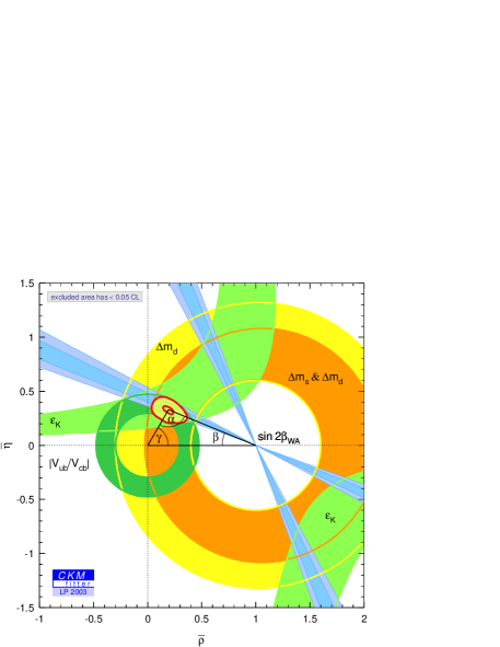
Figure 6: 95% c.l. constraints on the unitarity triangle from independent measurements in the kaon, $B_{d}^{0}$ and $B_{s}^{0}$ systems. The constraint from $\sin 2\beta$ has not been included in the fit, but is simply overlaid.

Note that the measurement of $\sin 2\beta=0.74$ [Eq. (6)] does not fix $2\beta$: both $2\beta=48^{\circ}$ and $132^{\circ}$ are allowed. In order to test the SM, we need to distinguish between these two solutions, i.e. $\cos 2\beta$ must be measured [19]. One possibility, discussed by T. E. Browder, A. Datta, P. J. O’Donnell and S. Pakvasa [20], is to study CP violation in $B\to D^{*+}D^{*-}K_{\scriptscriptstyle S}$ decays. Here both $\sin 2\beta$ and $\cos 2\beta$ can be obtained with some theoretical input [21].

The bottom line is that there are many ways of looking for physics beyond the SM through CP violation in the $B$ system. (Another method is discussed in Ref. [22].)

4 Measuring New-Physics Parameters

Suppose that some signal of physics beyond the SM is found in $B$ decays. Having confirmed the presence of new physics, we will want to identify it. Until recently, it was thought that this would have to wait for a high-energy collider such as the LHC, where the new particles can be produced directly. However, this is not necessarily true. As I will show below, it is possible to measure the NP parameters through CP violation in $B$ decays [23]. This knowledge will allow us to exclude certain NP models and will permit a partial identification of the NP, before the LHC.

New physics enters principally in loops in $B$ processes. In general, if NP is present in $B_{d}^{0}$–${\overline{B_{d}^{0}}}$ mixing, it will also affect ${\bar{b}}\to{\bar{d}}$ penguin amplitudes (and similarly for $B_{s}^{0}$–${\overline{B_{s}^{0}}}$ mixing and ${\bar{b}}\to{\bar{s}}$ penguins). As discussed in the previous section, at present there are several hints of new physics. All of these hints occur in processes involving ${\bar{b}}\to{\bar{s}}$ penguin diagrams — the ${\bar{b}}\to{\bar{d}}$ penguins appear to be unaffected. In line with this, we assume that NP is present only in ${\bar{b}}\to{\bar{s}}$ transitions. Furthermore, in order that the effects be measurable, we assume that the NP operators are roughly the same size as the SM penguin operators.

Assuming that the new physics affects ${\bar{b}}\to{\bar{s}}$ penguin transitions, it will lead to new effective ${\bar{b}}\to{\bar{s}}q{\bar{q}}$ operators. There are 20 possible NP operators $O_{\scriptscriptstyle NP}^{ij,q}\sim\bar{s}\Gamma_{i}b\,\bar{q}\Gamma_{j}q$ (here $\Gamma_{i,j}$ represent Lorentz structures; colour indices are suppressed). In general, there can be new weak and strong phases associated with each operator. A priori, the question of which operators are present is model-dependent. Performing a model-independent analysis therefore appears to be an intractable mess. Fortunately, it is possible to simplify things.

To see this, it is important to look at strong phases in more detail. In Sec. 2, I noted that strong phases are due to QCD processes. In particular, these phases are generated by rescattering. For example, in the SM, the strong phases of ${\bar{b}}\to{\bar{s}}s{\bar{s}}$ operators come principally from rescattering from the tree-level ${\bar{b}}\to{\bar{s}}c{\bar{c}}$ operators which have large CKM matrix elements. However, whereas the tree operator has Wilson coefficient $\sim 1$, the largest rescattered penguin operator has Wilson coefficient $\sim 0.05$. That is, the rescattered amplitude is $\sim 5\%$ as large as the amplitude causing the rescattering.

The new-physics strong phases are generated by rescattering from NP operators. However, the NP operators are only expected to be about as big as SM penguins. Thus, rescattered NP operators are only $\sim 5\%$ as large as this, which is quite small. It is therefore a reasonable approximation to neglect all NP rescattering. This implies that the NP strong phases are negligible relative to the SM strong phases.

The neglect of new-physics strong phases leads to a great simplification. The NP contributes to the decay $B\to f$ through the matrix elements $\left\langle f\right|O_{\scriptscriptstyle NP}^{ij,q}\left|B\right\rangle$. We denote each of the 20 NP ${\bar{b}}\to{\bar{s}}q{\bar{q}}$ matrix elements by $A_{i}e^{i\phi_{i}^{qq}}$, where $\phi_{i}^{qq}$ is the weak phase. The point is that we can now sum all of the contributions into a single effective NP matrix element:

$$\sum A_{i}e^{i\phi_{i}^{qq}}=A_{\scriptscriptstyle NP}^{qq}e^{i\Phi_{qq}}~{}.$$ (12)

In other words, for a given $b\to s{\bar{q}}q$ process ($q=u,d,s,c$), the effects of all NP operators can be parametrized in terms of a single effective NP amplitude $A_{\scriptscriptstyle NP}^{qq}$ and the corresponding weak phase $\Phi_{qq}$.

Furthermore, these NP parameters can be measured. Their knowledge will allow us to rule out many NP models, giving us a partial identification before LHC. There are several ways to make such measurements. I present one such method below. (It is similar to that used to extract $\gamma$ in the SM from $B_{d}^{0}(t)\to D^{(*)+}D^{(*)-}$ and $B_{d}^{0}\to D_{s}^{(*)+}D^{(*)-}$, described in Sec. 2.)

Consider the decay $B_{d}^{0}(t)\to\phi K_{\scriptscriptstyle S}$. In the SM, there is a single decay amplitude. This is a ${\bar{b}}\to{\bar{s}}s{\bar{s}}$ penguin, whose weak phase is zero. In the presence of NP, its amplitude can be written

$$A^{\prime}=P^{\prime}_{\scriptscriptstyle SM}e^{i\delta^{\prime}_{\scriptscriptstyle P}}+A_{\scriptscriptstyle NP}^{ss}e^{i\Phi_{ss}}~{}.$$ (13)

Assuming that the phase of $B_{d}^{0}$–${\overline{B_{d}^{0}}}$ mixing ($\beta$) is known independently, the above amplitude is described by 4 theoretical parameters: $P^{\prime}_{\scriptscriptstyle SM}$, $A_{\scriptscriptstyle NP}^{ss}$, $\delta^{\prime}_{\scriptscriptstyle P}$ and $\Phi_{ss}$. However, the measurement of the time-dependent rate for $B_{d}^{0}(t)\to\phi K_{\scriptscriptstyle S}$ yields only 3 observables. We therefore need to add theoretical input in order to extract all theoretical parameters.

This input comes from $B_{s}^{0}(t)\to\phi K_{\scriptscriptstyle S}$. This is a ${\bar{b}}\to{\bar{d}}s{\bar{s}}$ penguin decay, and therefore has no NP contributions. Its amplitude is

$$A=P_{u}e^{i\gamma}e^{i\delta_{u}}+P_{\scriptscriptstyle SM}e^{i\delta_{P}}~{}.$$ (14)

Here too there are 3 observables and 4 theoretical parameters. However, if we assume that $\gamma$ is known from independent non-${\bar{b}}\to{\bar{s}}$ measurements (e.g. $B\to DK$ decays), the measurement of this time-dependent rate allows us to extract $P_{\scriptscriptstyle SM}$, $P_{u}$ and $\delta\equiv\delta_{u}-\delta_{P}$. We can then obtain $P^{\prime}_{\scriptscriptstyle SM}$ using the SU(3) relation $\lambda P^{\prime}_{\scriptscriptstyle SM}/P_{\scriptscriptstyle SM}=1$. With this input, we can then extract $A_{\scriptscriptstyle NP}^{ss}$ and $\Phi_{ss}$.

To summarize: the above method allows us to measure the NP parameters $A_{\scriptscriptstyle NP}^{ss}$ and $\Phi_{ss}$. In fact, it is possible to obtain all $A_{\scriptscriptstyle NP}^{qq}$ and $\Phi_{qq}$ ($q=u,d,s,c$) similarly. (There are other methods as well which can be used to make such measurements [24].) This knowledge will allow us to distinguish among possible NP models. For example, some models (e.g. gluonic penguin operators with an enhanced chromomagnetic moment [25]) conserve isospin. In such models, one has $A_{\scriptscriptstyle NP}^{uu}=A_{\scriptscriptstyle NP}^{dd}$. Other models (e.g. $Z$- and $Z^{\prime}$-mediated flavour-changing neutral currents [26]) predict that the NP phase $\Phi_{qq}$ is universal. Finally, in general, the values of $A_{\scriptscriptstyle NP}^{qq}$ and $\Phi_{qq}$ found are process-dependent. However, some models (e.g. SUSY with R-parity breaking) predict that NP contributions to certain ${\bar{b}}\to{\bar{s}}q{\bar{q}}$ decays are process-independent. By measuring the NP parameters, all of these predictions can be tested. In this way we can exclude certain classes of NP models.

The bottom line is that, assuming that new physics is discovered through measurements of CP violation in the $B$ system, one can measure the NP parameters $A_{\scriptscriptstyle NP}^{qq}$ and $\Phi_{qq}$. Their knowledge will allow a partial identification of the NP, before its direct production at LHC.

5 Conclusions

To summarize: the raison d’être of $B$ physics is to find physics beyond the SM. There are many signals of new physics in measurements of CP violation in $B$ decays. Given a NP signal, it is possible to measure the NP parameters. This will allow a partial identification of the NP, before direct measurements at future high-energy colliders. Hopefully, we will find evidence of NP at $B$ factories, measure its parameters and (partially) identify it. Pat O’Donnell has contributed significantly to this endeavour.

References

- [1] K. Hagiwara et al. [Particle Data Group Collaboration], Phys. Rev. D 66, 010001 (2002), http://pdg.lbl.gov/pdg.html.
- [2] L. Wolfenstein, Phys. Rev. Lett. 51, 1945 (1983).
- [3] H. Albrecht et al. [ARGUS Collaboration], Phys. Lett. B 192, 245 (1987).
- [4] B. A. Campbell and P. J. O’Donnell, Phys. Rev. D 25, 1989 (1982).
- [5] The experimental data is tabulated by the Heavy Flavor Averaging Group, http://www.slac.stanford.edu/xorg/hfag/.
- [6] M. Gronau and D. London, Phys. Rev. Lett. 65, 3381 (1990).
- [7] M. Gronau and D. Wyler, Phys. Lett. B 265, 172 (1991); D. Atwood, I. Dunietz and A. Soni, Phys. Rev. Lett. 78, 3257 (1997). See also M. Gronau and D. London., Phys. Lett. B 253, 483 (1991); I. Dunietz, Phys. Lett. B 270, 75 (1991); N. Sinha and R. Sinha, Phys. Rev. Lett. 80, 3706 (1998).
- [8] A. Datta and D. London, Phys. Lett. B 584, 81 (2004).
- [9] D. Becirevic, invited talk at 2nd Workshop on the CKM Unitarity Triangle, Durham, England, April 2003, hep-ph/0310072.
- [10] E.g. see M. Imbeault, these proceedings.
- [11] J. P. Silva and L. Wolfenstein, Phys. Rev. D 49, 1151 (1994); M. Gronau, J. L. Rosner and D. London, Phys. Rev. Lett. 73, 21 (1994); O. F. Hernandez, D. London, M. Gronau and J. L. Rosner, Phys. Lett. B 333, 500 (1994); M. Gronau, O. F. Hernandez, D. London and J. L. Rosner, Phys. Rev. D 50, 4529 (1994), Phys. Rev. D 52, 6356 (1995), Phys. Rev. D 52, 6374 (1995).
- [12] See M. Gronau and J. L. Rosner, Phys. Lett. B 572, 43 (2003), and references therein.
- [13] See T. Hurth, E. Lunghi and W. Porod, hep-ph/0310282, and references therein.
- [14] See e.g. P. J. O’Donnell, Phys. Lett. B 175, 369 (1986); R. Grigjanis, P. J. O’Donnell, M. Sutherland and H. Navelet, Phys. Lett. B 213, 355 (1988) [Erratum-ibid. B 286, 413 (1992)], Phys. Rept. 228 (1993) 93.
- [15] A. Datta and D. London, arXiv:hep-ph/0303159.
- [16] A. Datta, H. J. Lipkin and P. J. O’Donnell, Phys. Lett. B 540, 97 (2002) [arXiv:hep-ph/0202235].
-
[17]
Talk by Jim Smith at Moriond, 2004:
http://moriond.in2p3.fr/QCD/2004/TuesdayMorning/Smith.pdf. -
[18]
This figure is taken from the CKMfitter group, see
http://www.slac.stanford.edu/xorg/ckmfitter/. -
[19]
BaBar has made a preliminary measurement of the
sign of through the time-dependent angular analysis of
. See talk by Marc Verderi at Moriond, 2004:
http://moriond.in2p3.fr/EW/2004/transparencies
/5_Friday/5_2_afternoon/5_2_2_Verderi/Verderi.pdf - [20] T. E. Browder, A. Datta, P. J. O’Donnell and S. Pakvasa, Phys. Rev. D 61, 054009 (2000).
- [21] See A. Datta, these proceedings.
- [22] V. Pagé, these proceedings.
- [23] A. Datta and D. London, arXiv:hep-ph/0404130.
- [24] A. Datta, M. Imbeault, D. London, V. Pagé, N. Sinha and R. Sinha, in preparation.
- [25] A. Kagan, Phys. Rev. D 51, 6196 (1995).
- [26] The model with -mediated FCNC’s was first introduced in Y. Nir and D. J. Silverman, Phys. Rev. D 42, 1477 (1990).