A Scaling Law for Quark Masses
and the CKM matrix

Abstract

We have recently argued that quark masses may follow a simple scaling law. In this paper we build a simple mass matrix for quarks that can reproduce the scaling law expression. The simple mass matrices of the model are then generalized through general rotations in the flavor space, including phase transformations. In turn they will be used to construct the quark-mixing matrix. It has been found that the model can predict the entries of the $CKM$ matrix in excellent agreement with current values. We give precise values for the light quark masses and determine the magnitude of the $CP$ violation and also the quark-mixing angles in the flavor space. The main motivation behind this work is to relate the scaling law predictions with quark-mixing, through a simple mass matrix and its generalized Hermitian form.

1 Introduction

Many of the observables in particle physics are related with broken symmetries. In this respect, the masses of the quarks could either be related with a Yukawa term, where the masses are due to a higgs scalar field coupling to fermions, or they can result as a departure from a chiral symmetry in the qcd sector. A remarkable feature of the quark masses is that they exhibit a clear hierarchy. We had discussed in a previous work  [1] that the quark masses might follow a simple scaling law;

$$\begin{split}&\frac{m_{t}}{m_{c}}=\epsilon^{2}_{u}\frac{m_{c}}{m_{u}}\\ \end{split}\ ,\ \ \ \ \ \ \ \begin{split}&\frac{m_{b}}{m_{s}}=\epsilon^{2}_{d}\frac{m_{s}}{m_{d}}\\ \end{split}$$ (1)

where we had initially considered the case $\epsilon_{u}=\epsilon_{d}=1$. It is well known that the u-type quark masses consistently satisfy the scaling expression for $\epsilon_{u}=1$. Unfortunately the scaling expression does not properly accommodate the d-type quark masses for $\epsilon_{d}=1$. If these scaling expressions are to make any sense at all, it is necessary to look for values of $\epsilon_{d}$ other than 1.

2 Scaling U-type Q-masses ($\epsilon_{u}=1$)

Let us first demonstrate that the u-type quark masses satisfy the scaling law expression for $\epsilon_{u}=1$. In this respect, we will use the currently known values of u-type quark masses. From the other side the simple scaling law makes sense only, if the quark masses are all renormalized at the same energy scale. Therefore for the u-type-quarks we choose the central value of $m_{t}=174.3\pm 5.1$ GeV as a useful scale. We choose for the c-quark mass $m_{c}(m_{c})=1.27\pm 0.05$ GeV given in [2], which rescales to $m_{c}{(m_{t})}=0.59$ GeV to $0.65$ GeV, using the QCD renormalization group [3] with $\Lambda=211^{+34}_{-30}$ MeV for five flavors  [4]. The u-mass $m_{u}$ is given as $m_{u}(1\,\text{GeV})=5.1\pm 0.9$ MeV [5]. Using the QCD renormalization group with $\Lambda=211^{+34}_{-30}$ MeV for five flavors, one has $m_{u}(m_{t})=1.87$ MeV to $2.68$ MeV.

A graphical approach based on the above summarized u-type quark masses would be very useful for the demonstration.

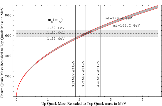
Figure 1: U-type quark masses falling into the dark region between the two curves satisfy the scaling law and the current bounds of u-type quark masses. Note that $m_{c}$ and $m_{u}$ axis are rescaled to $m_{t}=174.3$ GeV

Using the scaling law given in Eq.(1) we obtain for the charm quark mass, $m_{c}=\sqrt{m_{t}\,m_{u}}/\epsilon_{u}$. Since the top quark mass is known with a relatively good precision we can plot a relation between $m_{c}$ and $m_{u}$, once for the highest and once for the lowest values in $m_{t}=174.3\pm 5.1$ GeV. The plot is shown in Fig. (1). Along the curves the top quark mass is kept constant and the two curves correspond to the upper and lower limit in the t-quark mass which differ by the amount of $2*5.1$ GeV. The values of $m_{c}$ and $m_{u}$ falling into the region between the two, do automatically satisfy the scaling law. The current value of the c-quark mass from [2] is marked in the graphic as a grey stripe which lies between the dashed lines. The upper and lower dashed lines correspond to the highest and lowest values in $m_{c}{(m_{c})}=1.27\pm 0.05$ GeV. The intermediate dashed line in the grey region corresponds to the central value of $m_{c}{(m_{c})}=1.27$ GeV. These are the running masses in the $\overline{MS}$ scheme and the highest and lowest values are rescaled to $m_{c}{(m_{t})}=588$ MeV to $654$ MeV respectively. The current best value of u-quark masses given in [5] rescales to $m_{u}(m_{t})=1.87$ MeV to $2.68$ MeV and are marked in the graphic by the two vertical lines. These masses correspond to $m_{u}=3.33$ MeV and $4.76$ MeV at $2$ GeV as indicated in the figure. The vertical line intermediate to the other 2 vertical lines corresponds to $m_{u}=3.93$ MeV at 2 GeV. The darkest region which is the intersection of all the three regions, shows then the u-type quark masses which satisfy scaling law and which do simultaneously fall in the current limits of the u-type quark mass. The middle vertical and middle dashed line are quite well centered values with respect to the dark region.

3 Scaling D-type Q-masses ($\epsilon_{d}=\sqrt{2}$)

The same can be done for the d-type quarks. Among the d-type quarks $only$ the bottom quark is a ”heavy quark” and has a relatively well known mass. Unlike to the scale used in the former section ,the scaling of the d-type quarks will be done at $2$ GeV. For the bottom quark we choose $m_{b}(m_{b})=4.25\pm 0.10$ [2] which rescales to $m_{b}(2\,\text{GeV})=4.88$ GeV to $5.15$ GeV by using the QCD renormalization group with the current value $\Lambda=294^{+42}_{-38}$ MeV, for 4 flavors given in ”$\alpha_{s}$ 2002” by Bethke [4]. We chose for the strange quark mass $m_{s}(1\,\text{GeV})=175\pm 25$ MeV [5], which rescales to $m_{s}=114$ MeV to $153$ MeV at $2$ GeV by using the QCD renormalization group with the current value $\Lambda=336^{+42}_{-38}$ MeV, for 3 flavors given in  [4]. The down quark mass is chosen as $m_{d}(\text{1 GeV})=9.3\pm 1.4$ MeV [5] which rescales to $m_{d}=6.03$ MeV to $8.17$ MeV.

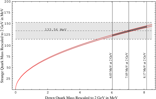
Figure 2: D-type quark masses falling into the dark region between the two curves satisfy the scaling law and current bounds of d-type quark masses for $\epsilon_{d}=\sqrt{2}$. Note that all values in the figure are rescaled to $2$ GeV.

Again it is useful to observe these values graphically. Using the scaling law given in Eq. (1) we obtain $m_{s}=\sqrt{m_{b}\,m_{d}}/\epsilon_{d}$. We can plot the relation as a function of the d-quark and s-quark masses once for the highest and once for the lowest values in $m_{b}(m_{b})=4.25\pm 0.10$ GeV. The output is illustrated in Fig. (2). D-type quark masses satisfying the scaling law, fall again between the two curves. The two curves again correspond to the upper and lower limit in the b-quark mass, which are respectively corresponding to $m_{b}(m_{b})=4.35$ GeV and $m_{b}(m_{b})=4.15$ GeV and are the running masses in the $\overline{MS}$ scheme. The grey stripe between the dashed lines marks the strange quark mass and corresponds to the interval $m_{s}(\text{1 GeV})=175\pm 0.25$ GeV, whose highest and lowest values are marked by the dashed lines, corresponding to $153$ MeV and $114$ MeV at $2$ GeV respectively. The d-quark mass $m_{d}=9.3\pm 1.4$ [5] is shown by the two vertical lines which correspond to $m_{d}=6.03$ MeV to $8.17$ MeV at $2$ GeV.

It is seen From the figure that the ranges for strange quark mass [5] and the d-quark mass [5] do have a common intersection with the region enclosed by the curves for $\epsilon_{d}=\sqrt{2}$, which is very well centered with respect to the limits.

If we repeat the procedure by drawing $m_{s}=\sqrt{m_{b}\,m_{d}}/\epsilon_{d}$ with $\epsilon_{d}=1$ in the figure, we would have obtained no overlap of the three regions. The constant b-quark mass curves for $\epsilon_{d}=1$ lie above those plotted in the figure.

4 The light Quark Sector

It is not possible to conclude that the scaling law is consistent with quark masses from the former two figures $alone$. One has to make sure that the light quark masses $m_{u},m_{s},m_{d}$ falling into the darg regions obey $also$ the bounds among light quark masses obtained from current algebra. To explore how the values of light quark masses are constrained by the scaling law, we consider the well known relations and bounds among light quark masses summarized in [6]:

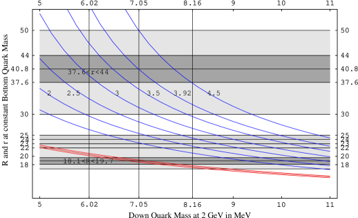
Figure 3: R and r ratios varied with respect to $m_{d}$ at $\epsilon=\sqrt{2}$. The dark grey stripes are the Leutwyler bounds and the light grey stripes are the bounds evaluated by the particle data group.

$$\begin{split}m_{u}/m_{d}&=0.553\pm 0.043\\ m_{s}/m_{d}&=18.9\pm 0.8\\ (m_{s}-\overline{m})/(m_{d}-m_{u})&=40.8\pm 3.2\\ \end{split}$$ (2)

Note that the error bars in the values are quite small, compared to the values evaluated by the particle data group in [7]. For the last two lines above we define the two coefficients $R,r$ which are frequently used to investigate the bounds on light quark masses

$$\begin{split}(i)\ \ \ \ \ &m_{s}/m_{d}=R\\ (ii)\ \ \ \ \ &(m_{s}-(m_{u}+m_{d})/2)/(m_{d}-m_{u})=r\\ \end{split}$$ (3)

These two ratios can be graphically investigated by eliminating $m_{s}$ with $\sqrt{m_{b}m_{d}}/\epsilon_{d}$, which follows from Eq. (1). For the ratio R, we will use again the upper and lower limits in $m_{b}$ as done before. For the ratio r, we use only the central value of $m_{b}$ and since r involves the u-quark mass, we highlight various $m_{u}$ values. These $m_{u}$ values are in turn subject to a consistency check with the scaling done for the u-type quark masses given in Fig (1). The variation of the value of $R$ with respect to $m_{d}$ and the variation of $r$ with respect to $m_{d}$ at various values of $m_{u}$ are shown together in Fig. (3) where both variations are coincided with a common $m_{d}$ axis. This is useful for selecting the consistent light quark masses. Note that the variation has been done so that the masses are constrained to exactly satisfy the scaling law.

Each of the curves in the upper half of the figure are giving the value of r, where again each separate curve corresponds to a different $m_{u}$ value at 2 GeV. These $m_{u}$ values are ranging from $1.5$ MeV to $4.5$ MeV, and are marked in the figure. Along all of these ”constant $m_{u}$” curves, the $central$ value of $m_{b}$ is also remaining constant, so that r is a function of $m_{d}$ for the specified $m_{u}$ and central $m_{b}$ mass.

The lower lying 3 adjacent curves are for $R$. Along these curves the b-quark mass is constant such that the upper one is for the upper limit of the b-quark mass, the lower one is for the lower limit and the middle one is for the central value.

Before we analyze this figure, we will introduce two other graphics which will be used in conjunction. The first shows the variation of the ratio $m_{u}/m_{d}$ with respect to the down quark mass $m_{d}$ and the second shows the variation of the mean value $\overline{m}=(m_{u}+m_{d})/2$ with respect to $m_{d}$ , again for various $m_{u}$ values that have been highlighted in fig. (3). These variations are shown in Fig. (4). The vertical lines in Fig. (4) correspond to the highest and lowest values in $m_{d}$ [5] at $2$ GeV and the dark grey stripe marks the highest and lowest values of $m_{u}/m_{d}$ given in Eq. (2). In Fig. (3) and (4) the light grey regions are pdg bounds evaluated by [7] [8] which we marked in the figures for keeping the discussion general. Indeed it is seen that these bounds in comparison to those given in Eq. (2) are containing huge error bars.

All figures in this work are produced so that they can be combined. Indeed the behavior of the scaling law is remarkable. Let us give an example: For a specific value of $R$ and $r$ we can pick up a value for the d-quark mass and a value for the u-quark mass from Fig. (3), then using this d-quark mass, the corresponding strange quark mass can be read off from Fig. (2) and the ratio $m_{u}/m_{d}$ and the mean value $\overline{m}$ can be read from Fig. (4). Finally the chosen $m_{u}$ value can be checked whether it is consistent with the scaling of the u-type quark masses in Fig. (1).

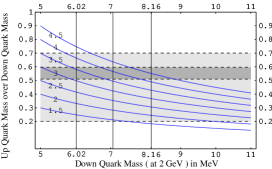
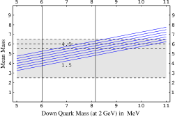
Figure 4: The ratio and the mean values of $m_{u}$ and $m_{d}$ are plotted as a function of the mass of the down quark. The curves correspond to various mass values of $m_{u}$ normalized to 2 GeV. The darkest regions is the current bound for the the ratio and the mean values provided by [6]. The lighter regions are bounds evaluated by [7][8]. Again for a specific value of $m_{d}$ the corresponding strange quark mass and R or r value that satisfy the scaling law can be read off from Fig.(2) and Fig.(3)

We summarize the light and heavy quark sector for $\epsilon_{d}=\sqrt{2}$ and $\epsilon_{u}=1$:

$$\begin{split}m_{s}&=133.56\ \ \ \ \ \ \text{MeV}\\ m_{d}&=7.05\ \ \ \ \ \ \ \ \ \text{MeV}\\ m_{u}&=3.92\ \ \ \ \ \ \ \ \ \text{MeV}\\ r&=40.98\\ R&=18.94\\ m_{u}/m_{d}&=0.556\\ m_{b}&=5.06\ \ \ \ \ \ \ \ \ \text{GeV}\\ \end{split}$$ (4)

These values are renormalized at 2 GeV. The bottom quark mass rescales to $m_{b}(m_{b})=4.28$ GeV. This perfect fitting might be an indication that $\epsilon=\sqrt{2}$ has a physical origin in the quark mass sector.

Using the values in eq.(4), we find for $m_{s}/\overline{m}$ and $m_{s}/m_{u}$ the values $24.34$ and $34.03$ respectively, which are also consistent with bounds $m_{s}/\overline{m}=24.4\pm 1.5$ and $m_{s}/m_{u}=34.4\pm 3.7$ respectively evaluated in [6].

Until now we used the Leutwyler and pdg bounds for quark masses as inputs, the scaling law alone has no predictive power. Suitable mass matrices that can give rise to such expressions might link the scaling law with the Yukawa sector and provide a deeper understanding. In the remaining part of the work we investigate this possibility.

5 A simple Model

The set of equations in (1) are reproducible from a simple Yukawa mass matrix which reads

$$M^{u}=\left[\begin{array}[]{ccc}k_{u}&0&a_{u}\epsilon_{u}^{\dagger}\\ 0&a_{u}&0\\ a_{u}\epsilon_{u}&0&0\\ \end{array}\right],\ \ \ \ \ \ \ \ \ \ M^{d}=\left[\begin{array}[]{ccc}k_{d}&0&a_{d}\epsilon_{d}^{\dagger}\\ 0&a_{d}&0\\ a_{d}\epsilon_{d}&0&0\\ \end{array}\right]$$ (5)

where we start with the assumption that $\mid\epsilon_{d}\mid\,>1$ and complex valued. Since $\epsilon_{u}=1$ was successful in scaling u-type quark masses it is not necessary to impose a similar condition on $\epsilon_{u}$. We also assume that $k_{u},a_{u}$ and $k_{d},a_{d}$ are real valued numbers. These simple mass matrices will be later on generalized. See also § 11 for equivalent simple mass matrices. We denote the corresponding diagonalized mass matrices with $\mathcal{M}^{u}$ and $\mathcal{M}^{d}$. The explicit form of the diagonal matrices are

$$\mathcal{M}^{u}=\left[\begin{array}[]{ccc}m_{u}&0&0\\ 0&m_{c}&0\\ 0&0&m_{t}\\ \end{array}\right],\ \ \ \ \ \ \ \ \ \ \mathcal{M}^{d}=\left[\begin{array}[]{ccc}m_{d}&0&0\\ 0&m_{s}&0\\ 0&0&m_{b}\\ \end{array}\right]$$ (6)

The quark masses above are expressible through the parameters $k_{u},a_{u}$ and $k_{d},a_{d}$ in the simple mass matrices as

$$\begin{split}m_{u}&=\frac{1}{2}\left[k_{u}-\sqrt{4\epsilon^{2}_{u}a^{2}_{u}+k^{2}_{u}}\right]\\ m_{c}&=a_{u}\\ m_{t}&=\frac{1}{2}\left[k_{u}+\sqrt{4\epsilon^{2}_{u}a^{2}_{u}+k^{2}_{u}}\right]\\ \end{split}\ \ \ \ \ \ \begin{split}m_{d}&=\frac{1}{2}\left[k_{d}-\sqrt{4\epsilon^{2}_{d}a^{2}_{d}+k^{2}_{d}}\right]\\ m_{s}&=a_{d}\\ m_{b}&=\frac{1}{2}\left[k_{d}+\sqrt{4\epsilon^{2}_{d}a^{2}_{d}+k^{2}_{d}}\right]\\ \end{split}$$ (7)

Here $\epsilon^{2}_{u}$ $=$ $\epsilon_{u}\epsilon^{\dagger}_{u}$. These are exact expressions and satisfy the simple scaling law regardless of the values of the parameters. That means, for all values of the parameters the mass ratios are as in Eq. (1). The parameters can be expressed in terms of quark masses using Eq. (7). The inverse transformations are

$$\begin{split}k_{u}&=m_{t}-m_{u}\ ,\\ a_{u}&=m_{c}\ ,\\ \end{split}\ \ \ \ \ \ \ \ \ \ \ \ \begin{split}k_{d}&=m_{b}-m_{d}\\ a_{d}&=m_{s}\\ \end{split}$$ (8)

Here it should be noted that $k_{u},k_{d}$ and $a_{u},a_{d}$ are positive. Therefore $m_{u}$ and $m_{d}$ carry a minus sign that follows from Eq. (7). Then $k_{u}$ is expressed as $m_{t}-m_{u}$ rather than $m_{t}+m_{u}$, while we assume that masses are positive quantities. From the other side since heavy quarks and light quarks lie in respectively GeV and MeV scales. The $central$ values of the parameters $k_{u},k_{d}$ receive some extra precision: So we have the possibility not to round the figures in the parameters up to 6 digits, which seems to be a useful and nice feature for evaluations in the CKM sector. However the quark masses have the appropriate figures. Note that $k_{u},k_{d}$ and $a_{u},a_{d}$ are rescaled in the $\overline{MS}$ scheme, so that the ratio of the masses remain constant.

In the following part of the work we will use the simple mass matrices to construct a satisfactory model for quark mixing. Let us continue with the construction of the model.

There is a transformation $V$ that diagonalizes our mass matrices $M$ such that $\mathcal{M}=V^{\dagger}MV$. The diagonalizing matrix V for the up and down simple mass matrices will be called $V^{u}$ and $V^{d}$ respectively. They are found as

$$V^{u}=\left[\begin{array}[]{ccc}\cos\beta_{1}&0&\sin\beta_{1}\\ 0&1&0\\ -\sin\beta_{1}&0&\cos\beta_{1}\\ \end{array}\right]\ \ \ \ \ V^{d}=\left[\begin{array}[]{ccc}\cos\beta_{2}&0&\sin\beta_{2}\\ 0&1&0\\ -\sin\beta_{2}&0&\cos\beta_{2}\\ \end{array}\right]$$ (9)

where the angles $\beta_{1}$ and $\beta_{2}$ are:

$$\beta_{1} =\cos^{-1}\left(-\frac{\sqrt{4\epsilon^{2}_{u}a^{2}_{u}+k^{2}_{u}-k_{u}\sqrt{4\epsilon^{2}_{u}a^{2}_{u}+k^{2}_{u}}}}{\sqrt{8\epsilon^{2}_{u}a^{2}_{u}+2\,k^{2}_{u}}}\right)$$ (10a)

$$\beta_{2} =\cos^{-1}\left(+\frac{\sqrt{4\epsilon^{2}_{d}a^{2}_{2}+k^{2}_{d}-k_{d}\sqrt{4\epsilon^{2}_{d}a^{2}_{2}+k^{2}_{d}}}}{\sqrt{8\epsilon^{2}_{d}a^{2}_{d}+2\,k^{2}_{d}}}\right)$$ (10b)

These are again exact expressions. The convention for the $\pm$ sign in $\beta_{1}$ and $\beta_{2}$ is discussed in § 9 and § 10. The resulting product $V^{u}{V^{d}}^{\dagger}$ is found as

$$V^{u}\,{V^{d}}^{\dagger}=V_{\beta_{1}}V_{\beta_{2}}^{\dagger}=V_{\delta}=\left[\begin{array}[]{ccc}\cos\delta&0&\sin\delta\\ 0&1&0\\ -\sin\delta&0&\cos\delta\\ \end{array}\right]$$ (11)

Here the angle $\delta=(\beta_{1}-\beta_{2})$. It is observed from the entries that this matrix is not capable of reproducing the CKM matrix [9] in this form. This does not imply that the simple mass matrices giving the scaled masses are $definetly$ useless. Indeed we have the freedom to rotate the Simple Mass Matrices in Eq. (5). It is seen from the $V$ matrices in Eq. (9) that we have so far only one angle for each of the up and down sectors. Indeed the generation space for each of the up and down quark species is 3 dimensional. It tells us that each of the simple mass matrices in Eq. (5) must be rotated further in 2 different Euler planes , so that each of the $V$ matrices additionally acquire two more angles, and produce an adequate expression for the CKM matrix. Therefore we introduce further rotations in the generation space. In the following it will be shown how the mass matrices can be brought to the most general form (containing 3 angles subject to diagonalization) while keeping the mass eigenvalues in Eq. (7) $intact$. After the Mass matrices are rotated into their final form we introduce the complex phases as described in § 6 and derive the corresponding $V$ matrices that fully describe the CKM matrix. The rotated mass matrices will be regarded as the $final$ mass matrices of the model and the simple mass matrices in Eq. (5) will be considered as special cases obtainable through setting the euler angles and complex phases to definite values as will be shown later.

In this respect let us define the following two transformation matrices in the generation space

$$V_{\alpha}=\left[\begin{array}[]{ccc}1&0&0\\ 0&\cos\alpha&\sin\alpha\\ 0&-\sin\alpha&\cos\alpha\\ \end{array}\right]\ \ \ \ \ \ \ \ \ \ V_{\gamma}=\left[\begin{array}[]{ccc}\cos\gamma&\sin\gamma&0\\ -\sin\gamma&\cos\gamma&0\\ 0&0&1\\ \end{array}\right]$$ (12)

Note that the subscript in $V$ defines the type of rotation by definition throughout the paper and is the argument of the sines and cosines. Using the first one, we can rotate the mass matrix $M^{u}$ into $V_{\alpha_{1}}^{\dagger}M^{u}V_{\alpha_{1}}$ and similarly $M^{d}$ into $V_{\alpha_{2}}^{\dagger}M^{d}V_{\alpha_{2}}$ with arbitrary angles $\alpha_{1}$ and $\alpha_{2}$. Now both resultant mass matrices preserve their initial mass eigenvalues as given in (7). The transformations that diagonalize the rotated mass matrices $V_{\alpha_{1}}^{\dagger}M^{u}V_{\alpha_{1}}$ and $V_{\alpha_{2}}^{\dagger}M^{d}V_{\alpha_{2}}$ can be reconstructed from $V^{u}$ and $V^{d}$ through the following method

$$\begin{split}\mathcal{M}^{u}&=\left[V_{-\alpha_{1}}V_{\beta_{1}}\right]^{\dagger}[V_{\alpha_{1}}^{\dagger}M^{u}V_{\alpha_{1}}]\left[V_{-\alpha_{1}}V_{\beta_{1}}\right]\\ \mathcal{M}^{d}&=\left[V_{-\alpha_{2}}V_{\beta_{2}}\right]^{\dagger}[V_{\alpha_{2}}^{\dagger}M^{d}V_{\alpha_{2}}]\left[V_{-\alpha_{2}}V_{\beta_{2}}\right]\\ \end{split}$$ (13)

where we use the fact that $V_{\alpha}V_{-\alpha}$ is a unit matrix and $V_{\alpha}^{\dagger}=V_{-\alpha}$. The modified diagonalizing transformations and modified mass matrices are then :

$$\begin{split}V^{u}&\rightarrow[V_{-\alpha_{1}}V_{\beta_{1}}],\\ V^{d}&\rightarrow[V_{-\alpha_{2}}V_{\beta_{2}}],\\ \end{split}\ \ \ \ \ \ \ \begin{split}M^{u}&\rightarrow V_{\alpha_{1}}^{\dagger}M^{u}V_{\alpha_{1}}\\ M^{d}&\rightarrow V_{\alpha_{2}}^{\dagger}M^{d}V_{\alpha_{2}}\\ \end{split}$$ (14)

and the resulting modified product for quark-mixing is

$$\begin{split}V^{u}{V^{d}}^{\dagger}&=[V_{-\alpha_{1}}V_{\beta_{1}}][V_{\beta_{2}}^{\dagger}V_{-\alpha_{2}}^{\dagger}]\\ &=[V_{-\alpha_{1}}V_{\beta_{1}-\beta_{2}}V_{\alpha_{2}}]\\ &=[V_{-\alpha_{1}}V_{\delta}V_{\alpha_{2}}]\\ \end{split}$$ (15)

In the last line we see that the term is now gradually improved with respect to that in Eq. (11). It contains now 4 angles. With the same token one can go a head and make use of $V_{\gamma}$. Using the set of Eqs. in (14) we perform a further rotation on the modified mass matrices this time applying $V_{\gamma}$. Then we obtain :

$$\begin{split}\mathcal{M}^{u}&=\left[V_{-\gamma_{1}}V_{-\alpha_{1}}V_{\beta_{1}}\right]^{\dagger}\left[V_{\gamma_{1}}^{\dagger}V_{\alpha_{1}}^{\dagger}M^{u}V_{\alpha_{1}}V_{\gamma_{1}}\right]\left[V_{-\gamma_{1}}V_{-\alpha_{1}}V_{\beta_{1}}\right]\\ \mathcal{M}^{d}&=\left[V_{-\gamma_{2}}V_{-\alpha_{2}}V_{\beta_{2}}\right]^{\dagger}\left[V_{\gamma_{2}}^{\dagger}V_{\alpha_{2}}^{\dagger}M^{d}V_{\alpha_{2}}V_{\gamma_{2}}\right]\left[V_{-\gamma_{2}}V_{-\alpha_{2}}V_{\beta_{2}}\right]\\ \end{split}$$ (16)

Here the modified mass matrices have preserved their mass eigenvalues as given in (7). The almost final transformation matrices diagonalizing these modified mass matrices above are collectively

$$\begin{split}V^{u}&\rightarrow V_{-\gamma_{1}}V_{-\alpha_{1}}V_{\beta_{1}}\ ,\\ V^{d}&\rightarrow V_{-\gamma_{2}}V_{-\alpha_{2}}V_{\beta_{2}}\ ,\\ \end{split}\ \ \ \ \ \ \ \ \ \begin{split}M^{u}&\rightarrow V_{\gamma_{1}}^{\dagger}V_{\alpha_{1}}^{\dagger}M^{u}V_{\alpha_{1}}V_{\gamma_{1}}\\ M^{d}&\rightarrow V_{\gamma_{2}}^{\dagger}V_{\alpha_{2}}^{\dagger}M^{d}V_{\alpha_{2}}V_{\gamma_{2}}\\ \end{split}$$ (17)

respectively. From Eq. (17), the almost final form of the CKM matrix can be written as

$$\begin{split}(V^{u})\,(V^{d})^{\dagger}&=\left[V_{-\gamma_{1}}V_{-\alpha_{1}}V_{\beta_{1}}\right]\left[V_{-\gamma_{2}}V_{-\alpha_{2}}V_{\beta_{2}}\right]^{\dagger}\\ &=V_{-\gamma_{1}}V_{-\alpha_{1}}V_{\beta_{1}}V_{\beta_{2}}^{\dagger}V_{-\alpha_{2}}^{\dagger}V_{-\gamma_{2}}^{\dagger}\\ &=V_{-\gamma_{1}}V_{-\alpha_{1}}V_{\delta}V^{\dagger}_{-\alpha_{2}}V^{\dagger}_{-\gamma_{2}}\\ &=V_{-\gamma_{1}}V_{-\alpha_{1}}V_{\delta}V_{\alpha_{2}}V_{\gamma_{2}}\\ \end{split}$$ (18)

It is seen at first sight that the six angles that meet each other in the expression induce an asymmetry. So we achieved the mentioned point. There are 6 angles in the CKM matrix and the rotated mass matrices generate the scaling law expression with the mass eigenvalues in Eq. (7). The simple mass matrices in Eq. (5) can be obtained by setting $\alpha_{1}=\alpha_{2}=\pi$ and $\gamma_{1}=\gamma_{2}=\pi$ in Eq. (17).

To enable a comparison with the standardized CKM matrix, we just let $\delta$ temporarily be zero, then $V_{\delta}$ becomes a unit matrix and we obtain

$$\left[\begin{array}[]{ccc}\cos\gamma_{1}&-\sin\gamma_{1}&0\\ \sin\gamma_{1}&\cos\gamma_{1}&0\\ 0&0&1\\ \end{array}\right]\left[\begin{array}[]{ccc}1&0&0\\ 0&\cos\epsilon&-\sin\epsilon\\ 0&\sin\epsilon&\cos\epsilon\\ \end{array}\right]\left[\begin{array}[]{ccc}\cos\gamma_{2}&\sin\gamma_{2}&0\\ -\sin\gamma_{2}&\cos\gamma_{2}&0\\ 0&0&1\\ \end{array}\right]$$

where we have rewritten the term $V_{-\alpha_{1}}V_{\alpha_{2}}$ as $V_{\epsilon}$ such that $\epsilon=(\alpha_{1}-\alpha_{2})$. The above form is equivalent to the standard form of the $CKM$ matrix given in [10]. If we consider the PDG version of the $CKM$ matrix [11] we see that it has 3 angles and a phase. We defined totally $2\,\alpha$’s, $2\,\gamma$’s and $2\,\beta$’s which makes totally 6 angles. It should be noted that this is not an over parametrization. Indeed the relative values count, this makes than 3 parameters. The extra phases that give rise to $CP$ violation will be introduced in a similar fashion in the next section. Here of course nothing prohibits us from fixing the 6 angles $(-\gamma_{1},-\alpha_{1},\beta_{1},-\beta_{2},\alpha_{2},\gamma_{2})$ to the experimental values. But the parameter $\delta$ is related with the quark masses and is not a completely free parameter. It is of interest whether $\delta$ will consistently predict the $CKM$ entries. In order to see the effect of $\delta$ on the entries, in the following part of the work we expand the expression in a series, for small angles. The expanded form is then adequate for a comparison with the Wolfenstein parametrization [12]. Let us first introduce the $CP$ violating phase in our model.

6 CP violating phase

During the construction of the $CKM$ matrix we had ignored the quark phases. A suitable way to incorporate the phases is to modify the mass matrices. We use the equations in (16) and introduce the quark phases

$$\begin{split}\mathcal{M}^{u}&=\left[V_{-\gamma_{1}}V_{-\alpha_{1}}V_{\phi_{1}}V_{\beta_{1}}\right]^{\dagger}\left[V_{\gamma_{1}}^{\dagger}V_{\alpha_{1}}^{\dagger}V_{\phi_{1}}M^{u}V_{\phi_{1}}^{\dagger}V_{\alpha_{1}}V_{\gamma_{1}}\right]\left[V_{-\gamma_{1}}V_{-\alpha_{1}}V_{\phi_{1}}V_{\beta_{1}}\right]\\ \mathcal{M}^{d}&=\left[V_{-\gamma_{2}}V_{-\alpha_{2}}V_{\phi_{2}}V_{\beta_{2}}\right]^{\dagger}\left[V_{\gamma_{2}}^{\dagger}V_{\alpha_{2}}^{\dagger}V_{\phi_{2}}M^{d}V_{\phi_{2}}^{\dagger}V_{\alpha_{2}}V_{\gamma_{2}}\right]\left[V_{-\gamma_{2}}V_{-\alpha_{2}}V_{\phi_{2}}V_{\beta_{2}}\right]\\ \end{split}$$ (19)

The middle terms in the brackets $[...]$ are the $final$ mass Matrices for up and down quarks. A suitable choice for the transformations $V_{\phi_{2}}$ and $V_{\phi_{1}}$ might be simply a diagonal matrix with quark phases as entries

$$V_{\phi_{1}}=\left[\begin{array}[]{ccc}e^{i\,\phi_{u}}&0&0\\ 0&e^{i\,\phi_{c}}&0\\ 0&0&e^{i\,\phi_{t}}\\ \end{array}\right]\ \ \ \ \ \ \ \ \ \ V_{\phi_{2}}=\left[\begin{array}[]{ccc}e^{i\,\phi_{d}}&0&0\\ 0&e^{i\,\phi_{s}}&0\\ 0&0&e^{i\,\phi_{b}}\\ \end{array}\right]$$ (20)

The expressions for the diagonalizing transformations $V^{u}$ and $V^{d}$ are now containing the phase information as well. The final form of the $V$ matrices and mass matrices are :

$$\begin{split}V^{u}&\rightarrow V_{-\gamma_{1}}V_{-\alpha_{1}}V_{\phi_{1}}V_{\beta_{1}},\\ V^{d}&\rightarrow V_{-\gamma_{2}}V_{-\alpha_{2}}V_{\phi_{2}}V_{\beta_{2}},\\ \end{split}\ \ \ \ \ \ \ \ \ \begin{split}M^{u}&\rightarrow V_{\gamma_{1}}^{\dagger}V_{\alpha_{1}}^{\dagger}V_{\phi_{1}}M^{u}V_{\phi_{1}}^{\dagger}V_{\alpha_{1}}V_{\gamma_{1}}\\ M^{d}&\rightarrow V_{\gamma_{2}}^{\dagger}V_{\alpha_{2}}^{\dagger}V_{\phi_{2}}M^{d}V_{\phi_{2}}^{\dagger}V_{\alpha_{2}}V_{\gamma_{2}}\\ \end{split}$$ (21)

The $CKM$ matrix in our model takes its final form as

$$\begin{split}(V^{u})\,(V^{d})^{\dagger}&=U^{CKM}=V_{-\gamma_{1}}V_{-\alpha_{1}}V_{\phi_{1}}V_{\delta}{V_{\phi_{2}}}^{\dagger}V_{\alpha_{2}}V_{\gamma_{2}}\\ \end{split}$$ (22)

Note that when we temporarily set $\delta$ and $\gamma_{2}$ to zero and collect $V_{\phi_{1}}$ and $V^{\dagger}_{\phi_{2}}$ in a single expression with one non-vanishing phase such that $V_{\phi_{1}}V^{\dagger}_{\phi_{2}}=diag[1,1,e^{i\,(\phi_{t}-\phi_{b})}]$, then we obtain a rather standard form.

$$\small\left[\begin{array}[]{ccc}c_{\gamma_{1}}&-s_{\gamma_{1}}&0\\ s_{\gamma_{1}}&c_{\gamma_{1}}&0\\ 0&0&1\\ \end{array}\right]\left[\begin{array}[]{ccc}1&0&0\\ 0&c_{\alpha_{1}}&-s_{\alpha_{1}}\\ 0&s_{\alpha_{1}}&c_{\alpha_{1}}\\ \end{array}\right]\left[\begin{array}[]{ccc}1&0&0\\ 0&1&0\\ 0&0&e^{i\phi_{tb}}\\ \end{array}\right]\left[\begin{array}[]{ccc}c_{\gamma_{2}}&s_{\gamma_{2}}&0\\ -s_{\gamma_{2}}&c_{\gamma_{2}}&0\\ 0&0&1\\ \end{array}\right]$$

where we shortly denote $\phi_{tb}=\phi_{t}-\phi_{b}$. This shows how close our model stands to the standardized form. The main difference stems from $\delta$ as discussed before, which is determinable from quark masses and the phases $\phi_{u},\phi_{c},\phi_{t},$ and $\phi_{d},\phi_{s},\phi_{b}$ which follow from observable $CP$ violation.

7 Predicting the CKM entries

At the first stage we are interested in what influence $V_{\delta}$ might have. We use the quark masses summarized in §(3) , §(2) and §(4) to determine the parameters $k_{u},a_{u}$ and $k_{d},a_{d}$ given in Eq.(8) and subsequently insert them into Eq.(10a) and into Eq. (10b) to obtain $\beta_{1}$ and $\beta_{2}$. It is remarkable that these values appear as small deviations around $\frac{\pi}{2}$. This is discussed in §9 and §10. As $\beta_{1}$ and $\beta_{2}$ are small, $\delta$ will also be small. We obtain $\delta=\beta_{1}-\beta_{2}=0.040868$. Here the precision comes from the unrounded figures in $k_{u},k_{d}$, which was discussed before. Let us start with

$$\begin{split}(V^{u})\,(V^{d})^{\dagger}&=U^{CKM}=V_{-\gamma_{1}}V_{-\alpha_{1}}V_{\phi_{1}}V_{\delta}{V_{\phi_{2}}}^{\dagger}V_{\alpha_{2}}V_{\gamma_{2}}\\ \end{split}$$ (23)

For explicit calculations, the matrices $V_{-\gamma_{1}}$ , $V_{-\alpha_{1}}$ ,$V_{\alpha_{2}}$ and $V_{\gamma_{2}}$ are defined as in Eq. (12) and $V_{\delta}$ is given in Eq. (11). With some trial we choose for the parameters,

$$\begin{array}[]{lcrcr}\gamma_{1}&=&\frac{\pi}{2}+0.226580&=&\frac{\pi}{2}+\Delta_{\gamma_{1}}\\ \gamma_{2}&=&\frac{\pi}{2}+0.003000&=&\frac{\pi}{2}+\Delta_{\gamma_{2}}\\ \alpha_{1}&=&0+0.030000&=&0+\Delta_{\alpha_{1}}\\ \alpha_{2}&=&0+0.022658&=&0+\Delta_{\alpha_{2}}\\ \beta_{1}&=&\frac{\pi}{2}+0.003557&=&\frac{\pi}{2}-\Delta_{\beta_{1}}\\ \beta_{2}&=&\frac{\pi}{2}-0.037312&=&\frac{\pi}{2}-\Delta_{\beta_{2}}\\ \end{array}$$ (30)

Where the $\Delta$ ’s denote the amount of deviation from the central values. We simply substitute these values in eq.(23). The absolute values are found as

$$\left[\begin{array}[]{lll}0.974867&0.222759&0.003651\\ 0.222640&0.974017&0.041505\\ 0.008155&0.040859&0.999132\\ \end{array}\right]$$ (31)

Where a complex phase $\phi_{c}=0.144$ has been used, while all other phases are set identically to zero. The above values of the parameters reproduce the $CKM$ entries in an excellent agreement with the current values [11].

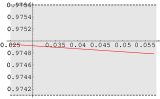
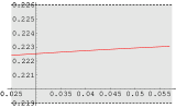
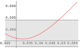
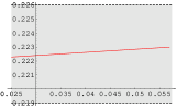
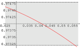
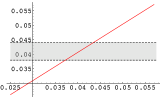
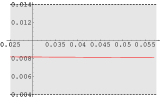
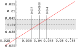
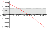
Figure 5: Variation of $CKM$ entries with respect to $\delta$, the position of each figure overlaps with its position in the $CKM$ matrix.

Slight changes are possible through changing the central values of the angles at fixed $\delta=0.040868$. Whether the model contains any triviality with respect to the parameter $\delta$ could be clarified by investigating the effect of $\delta$ on the $CKM$ entries. For example would it be possible to fix the angles $(-\gamma_{1},-\alpha_{1},\alpha_{2},\gamma_{2})$ so that they give the current $CKM$ values regardless of what value $\delta$ takes ?

A graphical approach shows that the central values of the $CKM$ entries are reproducible only within a very narrow band for $\delta$ which lies approximately in the range $0.037<\delta<0.044$. This fact is illustrated in fig. (5) where all other parameters are kept fixed as in Eq. (30), but only $\delta$ is varied over a large interval, starting from $0.025$ up to $0.057$. Indeed this interval is too large and will produce bad quark masses as we depart from the central value: $\delta=0.040868$. As seen from the figures, the entries $V_{ts}$ ,$V_{cb}$ , $V_{tb}$ are largely $\delta$ dependent. The grey regions are current bounds for the entries. Again from the variation of the CKM entries with respect to $\delta$, we see that the bound on $\delta$ is largely imposed by the $V_{ts}$ ,$V_{cb}$ , $V_{tb}$ entries. The best values are in the interval $0.037<\delta<0.044$. This means that the better these entries are known the more feedback is obtained for determining quark masses. Our previous analysis for quark masses gave a rather good value.i.e., $\delta=0.040868$ which is both consistent with the $CKM$ entries and quark masses. It also allows a total phase of $\phi_{c}=0.144$ which is consistent. We consider as next the variation of the $CKM$ entries with respect to the phases $(\phi_{u},\phi_{c},\phi_{t})$ at constant values of the parameters as given in Eq. (30).

Case A :

The variation of $CKM$ entries with respect to $\phi_{c}$ in the large interval $-0.6<\phi_{c}<0.6$ are shown in Fig. (6). Here all other phases are set identically to zero.

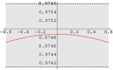
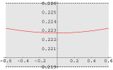
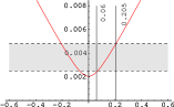
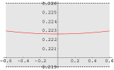
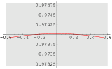
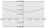
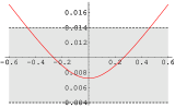
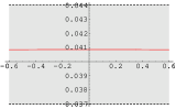
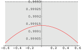
Figure 6: Variation of the $CKM$ entries with respect to $\phi_{c}$, the position of each figure overlaps with its position in the $CKM$ matrix.

It is seen that $V_{ub}$ and $V_{td}$ are largely $\phi_{c}$ dependent. The determination of the $CP$ violating phase is therefore predictable from precise measurements of these entries. The current range for $V_{ub}$ which is $0.0025\dots 0.0048$ constrains $\phi_{c}$ to vary between $0.06<\phi_{c}<0.205$ as seen from the figure.

Case B :

Let us set all phases to zero and vary this time $\phi_{u}$ in the interval $-0.6<\phi_{u}<06$. Again the current value of $V_{ub}$ constrains $\phi_{u}$ to vary between $0.177<\phi_{u}<0.543$ as seen from the figure.

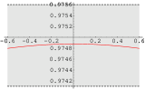
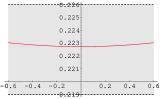
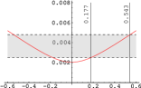
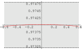
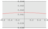
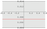
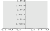
Figure 7: Variation of $CKM$ entries w.r.t the parameter $\phi_{u}$, the position of each figure overlaps with its position in the $CKM$ matrix.

Case C :

A final case that we illustrate is where only $\phi_{t}$ is varied. Again all other phases are set to zero and we vary $\phi_{t}$ in the range $-0.6<\phi_{t}<0.6$. This time the current value of $V_{ub}$ severely constrains $\phi_{t}$ to the interval $0.046<\phi_{t}<0.142$ as seen from the figure.

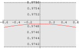
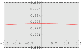
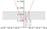
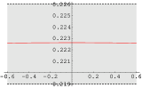
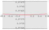
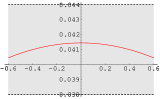
Figure 8: Variation of $CKM$ entries w.r.t the parameter $\phi_{t}$, the position of each figure overlaps with its position in the $CKM$ matrix.

It is seen from the three cases that the phases have different contributions on the entries. If we assume that the central values $(-\gamma_{1},-\alpha_{1},\beta_{1},$ $\beta_{2},\alpha_{2},\gamma_{2})$ given in eq. (30) are good values, we can expand the expression in Eq. (23) in a series around these values where $\Delta$’s appear as fluctuations shown in the second column of Eq. (30).

8 Fluctuations

To make the analysis some what easier, we let the complex phases be initially zero and expand the $U^{CKM}$ around the central values. If only the second order terms are selected then we obtain:

$$\scriptsize V_{r}\approx\left[\begin{array}[]{ccc}1-\frac{1}{2}(\alpha_{1}-\alpha_{2})^{2}-\frac{1}{2}(\Delta_{\gamma_{1}}-\Delta_{\gamma_{2}})^{2}&-\Delta_{\gamma_{1}}+\Delta_{\gamma_{2}}-\alpha_{1}\,\delta&+\alpha_{1}-\alpha_{2}-\Delta_{\gamma_{1}}\,\delta\\ \vspace{1mm}\hfil\\ +\Delta_{\gamma_{1}}-\Delta_{\gamma_{2}}+\alpha_{2}\,\delta&1-\frac{1}{2}(\Delta_{\gamma_{1}}-\Delta_{\gamma_{2}})^{2}-\frac{1}{2}\delta^{2}&+(\alpha_{1}-\alpha_{2})\Delta_{\gamma_{1}}+\delta\\ \vspace{1mm}\hfil\\ -\alpha_{1}+\alpha_{2}+\Delta_{\gamma_{2}}\,\delta&+(\alpha_{2}-\alpha_{1})\Delta_{\gamma_{2}}-\delta&1-\frac{1}{2}(\alpha_{1}-\alpha_{2})^{2}-\frac{1}{2}\delta^{2}\\ \end{array}\right]$$

The entries come out rather interesting. At second order, we see how the diagonal elements start to differ from each other through $\delta$. And it is also seen how $\delta$ induces an asymmetry between off diagonal terms. Parameterizing the $CKM$ matrix with respect to the phases will bring changes in the terms. Let us take the most general case where all phases fluctuate around zero up to second order, then $V_{\phi_{1}}$ and $V_{\phi_{2}}$ will contribute to all entries above. The new terms which additively contribute to each side will be collected in the following matrix

$$V_{c}=\left[\begin{array}[]{lll}V_{11}&V_{12}&V_{13}\\ V_{21}&V_{22}&V_{23}\\ V_{31}&V_{32}&V_{33}\\ \end{array}\right]$$ (32)

where by definition all second order terms are collected in $V=V_{r}+i\,V_{c}$. The terms in the above matrix $V_{c}$ come out as

$$\begin{split}V_{11}&=-\frac{1}{2i}(\phi_{c}-\phi_{s})^{2}-(\phi_{s}-\phi_{c})\\ V_{22}&=-\frac{1}{2i}(\phi_{d}-\phi_{u})^{2}-(\phi_{d}-\phi_{u})\\ V_{33}&=-\frac{1}{2i}(\phi_{b}-\phi_{t})^{2}-(\phi_{b}-\phi_{t})\\ \end{split}$$

$$\begin{split}V_{12}&=+\gamma_{2}(\phi_{c}-\phi_{s})+\gamma_{1}(\phi_{d}-\phi_{u})\\ V_{21}&=+\gamma_{1}(\phi_{c}-\phi_{s})+\gamma_{2}(\phi_{d}-\phi_{u})\\ V_{13}&=-\alpha_{2}(\phi_{c}-\phi_{s})+\alpha_{1}(\phi_{b}-\phi_{t})\\ V_{31}&=-\alpha_{1}(\phi_{c}-\phi_{s})+\alpha_{2}(\phi_{b}-\phi_{t})\\ V_{23}&=-\delta(\phi_{b}-\phi_{u})\\ V_{32}&=+\delta(\phi_{d}-\phi_{t})\\ \end{split}$$ (33)

If each quark in an isospin pair has the same phase then up to second order we see from the above expressions that the phase contributions identically vanish. We have a non-vanishing complex phase only if the quarks in an isospin pair have different phases. Then only one unequal phase pair is sufficient to induce $CP$ violation. Using the following definitions:

$$\begin{split}\phi_{ud}&=\phi_{u}-\phi_{d}\\ \phi_{cs}&=\phi_{c}-\phi_{s}\\ \phi_{tb}&=\phi_{t}-\phi_{b}\\ \end{split}$$ (34)

the over all amount of phase $\Phi$ for any choice of $(-\gamma_{1},-\alpha_{1},\delta,\alpha_{2},\gamma_{2})$ could be calculated from the determinant of the $CKM$ matrix and comes out as

$$\begin{split}\Phi&=e^{-i(\phi_{ud}+\phi_{cs}+\phi_{tb})}\\ \end{split}$$ (35)

It is definitely better and more practical to use the exact form of the $CKM$ matrix given in Eq. (22) rather than the parameterized form. Since even at second order, certain entries deviate from their exact values in a few factors of $10^{-3}$ and although third order contributions are a good cure they do create a mess. The main reason we have parameterized our expression is to visualize the behavior of the entries. Indeed a similar behavior is well known from the Wolfenstein parametrization where the usual $\lambda^{3}$ , $\rho$ and $\eta$ terms are inevitable.

9 The Massless Limit

It is remarkable that $\beta_{1}$ and $\beta_{2}$ take values which are small deviations around $\frac{\pi}{2}$ and simultaneously predict acceptable quark masses. Let us turn the deviations $\Delta_{\beta_{1}}$ and $\Delta_{\beta_{2}}$ temporarily off by setting them to zero. Recalling the expression in Eq. (10a) and (10b) we get

$$\beta_{2}=\cos^{-1}\left[+\frac{\sqrt{4\epsilon^{2}_{d}a^{2}_{d}+k^{2}_{d}-k_{d}\sqrt{4\epsilon^{2}_{d}a^{2}_{d}+k^{2}_{d}}}}{\sqrt{8\epsilon^{2}_{d}a^{2}_{d}+2\,k^{2}_{d}}}\right]\rightarrow\frac{\pi}{2}$$ (36)

The argument of $\cos^{-1}[\dots]$ becomes zero, which implies $a_{d},k_{d}\rightarrow 0$. This is obviously the massless limit. Note that $k_{d}$ does not necessarily have to be zero for $\beta_{2}$ to become $\pi/2$. But it has to be zero so that the third family receives no mass in the discussed limit. The similar applies to $\beta_{1}$ and gives $a_{u},k_{u}\rightarrow 0$. This is totaly consistent with the notion of symmetry breaking. The masses result from a relatively small deviation from an angle. But when we set $\delta$ identically to zero we see from the expression $V_{r}$ that still we have non zero entries, in the case that one of the following asymmetry exists: $\gamma_{1}\neq\gamma_{2}$, $\alpha_{1}\neq\alpha_{2}$, $\phi_{u}\neq\phi_{d}$, $\phi_{c}\neq\phi_{s}$, $\phi_{b}\neq\phi_{t}$. There is nothing contradictory about this fact, since in the very first step of the construction if $a_{u}$ , $a_{d}$ and $k_{u}$ , $k_{d}$ are set to zero then the mass matrices do vanish, and all parameters go symmetric.

10 The Degenerate Mass Limit

The $\pm$ sign convention in the angles $\beta_{1}$ and $\beta_{2}$ is easily clarified when certain limits of the parameters in the simple mass matrices are considered. As a first case we consider the degenerate mass limit where one has

$$\frac{m_{u}}{\epsilon_{u}}=m_{c}=\frac{m_{t}}{\epsilon_{u}}=\frac{m_{d}}{\epsilon_{d}}=m_{s}=\frac{m_{b}}{\epsilon_{d}}$$ (37)

This spectrum can be achieved by setting $k_{u}=k_{d}=0$ and $a_{u}=a_{d}$ $\neq 0$. A second possibility is

$$\frac{m_{u}}{\epsilon_{u}}=m_{c}=\frac{m_{t}}{\epsilon_{u}}\neq\frac{m_{d}}{\epsilon_{d}}=m_{s}=\frac{m_{b}}{\epsilon_{d}}$$ (38)

This degenerate mass spectrum could be obtained through setting $k_{u}=k_{d}=0$ and $a_{u}\neq 0$ $,a_{d}\neq 0$ and $a_{u}\neq a_{d}$. For the first case we have then

$$\begin{split}\beta_{1}&=\cos^{-1}\left[-\frac{\sqrt{4\epsilon^{2}_{u}a^{2}_{u}+k^{2}_{u}-k_{u}\sqrt{4\epsilon^{2}_{u}a^{2}_{u}+k^{2}_{u}}}}{\sqrt{8\epsilon^{2}_{u}a^{2}_{u}+2\,k^{2}_{u}}}\right]\rightarrow\frac{3\pi}{4}\\ \beta_{2}&=\cos^{-1}\left[+\frac{\sqrt{4\epsilon^{2}_{d}a^{2}_{2}+k^{2}_{d}-k_{d}\sqrt{4\epsilon^{2}_{d}a^{2}_{2}+k^{2}_{d}}}}{\sqrt{8\epsilon^{2}_{d}a^{2}_{d}+2\,k^{2}_{d}}}\right]\rightarrow\frac{\pi}{4}\\ \end{split}$$ (39)

and consequently $\delta=\beta_{1}-\beta_{2}\rightarrow\pi/2$ which gives for the matrix $V_{\delta}$

$$\ V_{\beta_{1}}V_{\beta_{2}}^{\dagger}=V_{\delta}=\left[\begin{array}[]{ccc}0&0&1\\ 0&1&0\\ -1&0&0\\ \end{array}\right]$$ (40)

The point of the discussion lies exactly here. If there were no minus sign in $\beta_{1}$ , $\delta$ would go to zero and $V_{\delta}$ would become a unit matrix. The minus sign is essential since when one lets all angles go symmetric like $\alpha_{1}=\alpha_{2}\neq 0$, $\gamma_{1}=\gamma_{2}\neq 0$, then we still have mixing as should be expected. If the minus sign were not present in Eq. (39), the CKM matrix would have turned into a unit matrix for $\alpha_{1}=\alpha_{2}\neq 0$, $\gamma_{1}=\gamma_{2}\neq 0$. Therefore we choose for $\beta_{1}$ and $\beta_{2}$ opposite signs.

The second case for degenerate quark masses is indeed not that much a special case. Here $\delta$ will depend on $a_{u}$ , $a_{d}$ and other angles as well but the sign convention should be of course as in the first case.

A final case of interest is when one has $\alpha_{1}=\alpha_{2}=\gamma_{2}=\pi/2$. This decouples the third family from the first two.

11 The Nature of the Scaling law

For the 3 families $\Psi_{1}$,$\Psi_{2}$ and $\Psi_{3}$, we have initially introduced the mass matrix

$$M=\left[\begin{array}[]{ccc}k&0&a\\ 0&a&0\\ a&0&0\\ \end{array}\right]_{1}$$ (41)

where for generality the isospin up and down indices are suppressed. This matrix produces the scaled masses. It is possible to construct other matrices with 3 entries of ’a’ and one ’k’ that produces the same eigenvalues as well. Now if we impose a permutation on the family index such that $\Psi_{1}$ is interchanged with $\Psi_{2}$, keeping $\Psi_{3}$ untouched we perform a map on the entries of the mass matrix

$$\begin{array}[]{c}M_{11}=k\\ M_{22}=a\\ M_{31}=a\\ M_{13}=a\\ \end{array}\mapsto\begin{array}[]{c}M_{22}=k\\ M_{11}=a\\ M_{32}=a\\ M_{23}=a\\ \end{array}$$ (42)

one can generate the matrix

$$M=\left[\begin{array}[]{ccc}a&0&0\\ 0&k&a\\ 0&a&0\\ \end{array}\right]_{2}$$ (43)

which has the same eigenvalues with the initial one ,but is not identical which means that the mass matrix has no symmetry property under this permutation. There are four more cases which are through permutation obtainable

$$\left[\begin{array}[]{ccc}0&0&a\\ 0&a&0\\ a&0&k\\ \end{array}\right]_{3}\ ,\left[\begin{array}[]{ccc}a&0&0\\ 0&0&a\\ 0&a&k\\ \end{array}\right]_{4}\ ,\left[\begin{array}[]{ccc}k&a&0\\ a&0&0\\ 0&0&a\\ \end{array}\right]_{5}\ ,\left[\begin{array}[]{ccc}0&a&0\\ a&k&0\\ 0&0&a\\ \end{array}\right]_{6}$$ (44)

These are all the six possible simple mass matrices that produce the scaled masses. Non of these 6 matrices are identical and the mass matrix has obviously no permutation symmetry. We have chosen especially the first one while the the mass eigenvalues are ordered from low to high i.e., $(m_{u},m_{c},m_{t})$. The point in this discussion is that the two mass matrices with label 1 and 3 can be rotated with matrices of type $V_{\beta}$ to their diagonal form. The matrices 2 and 4 can be diagonalized with $V_{\alpha}$ and the remaining two can be diagonalized through $V_{\gamma}$. Any of the above mass matrices can be used to build the $CKM$ matrix with same technique to obtain equivalent descriptions. If $k$ is set in all 6 matrices to zero, we obtain a degenerate mass spectrum i.e., $(-a,a,a)$, which is not describing our(!) quarks. Presumably the scaling law is the simplest natural extension of the degenerate case with the inclusion of the parameter $k$.

12 Generating the Texture

The generalized transformations in the flavor space which we based on the scaling law, do naturally define a texture. We will look at the mass matrices given in eq. (19) and reduce it to a Texture. The mass matrices are

$$\begin{split}\mathbb{M}^{u}&=V_{\gamma_{1}}^{\dagger}V_{\alpha_{1}}^{\dagger}V_{\phi_{1}}M^{u}V_{\phi_{1}}^{\dagger}V_{\alpha_{1}}V_{\gamma_{1}}\\ \mathbb{M}^{d}&=V_{\gamma_{2}}^{\dagger}V_{\alpha_{2}}^{\dagger}V_{\phi_{2}}M^{d}V_{\phi_{2}}^{\dagger}V_{\alpha_{2}}V_{\gamma_{2}}\\ \end{split}$$ (45)

First we consider the phaseless case, where all quark phases are identically set to zero so that $V_{\phi_{1}}=V_{\phi_{2}}=I$. Using the explicit expression for the $V$ matrices the mass matrices $\mathbb{M}^{u}$ and $\mathbb{M}^{d}$ come out as.

$$\left[\begin{array}[]{ccc}F_{u}&A_{u}&E_{u}\\ A_{u}&C_{u}&B_{u}\\ E_{u}&B_{u}&D_{u}\\ \end{array}\right]\ \ \ \ ,\ \ \ \ \ \left[\begin{array}[]{ccc}F_{d}&A_{d}&E_{d}\\ A_{d}&C_{d}&B_{d}\\ E_{d}&B_{d}&D_{d}\\ \end{array}\right]$$ (52)

where the entries are explicitly

$$\begin{split}A_{u}&=a_{u}\,s_{\alpha_{1}}\left(\epsilon_{u}s^{2}_{\gamma_{1}}-\epsilon^{\dagger}_{u}c^{2}_{\gamma_{1}}\right)+\left(k_{u}-a_{u}c^{2}_{\alpha_{1}}\right)s_{\gamma_{1}}c_{\gamma_{1}}\\ B_{u}&=a_{u}\,c_{\alpha_{1}}\left(\epsilon_{u}s_{\gamma_{1}}+s_{\alpha_{1}}c_{\gamma_{1}}\right)\\ C_{u}&=a_{u}\,c^{2}_{\alpha_{1}}c^{2}_{\gamma_{1}}-\,a_{u}s_{2\gamma_{1}}s_{\alpha_{1}}Re[\epsilon_{u}]+k_{u}s^{2}_{\gamma_{1}}\\ D_{u}&=a_{u}\,s^{2}_{\alpha_{1}}\\ E_{u}&=a_{u}\,c_{\alpha_{1}}\left(\epsilon_{u}c_{\gamma_{1}}-s_{\alpha_{1}}s_{\gamma_{1}}\right)\\ F_{u}&=k_{u}\,c^{2}_{\gamma_{1}}+a_{u}c^{2}_{\alpha_{1}}s^{2}_{\gamma_{1}}+a_{u}s_{\alpha_{1}}s_{2\gamma_{1}}Re[\epsilon_{u}]\\ \end{split}$$ (53)

$$\begin{split}A_{d}&=a_{d}\,s_{\alpha_{2}}\left(\epsilon_{d}s^{2}_{\gamma_{2}}-\epsilon^{\dagger}_{d}c^{2}_{\gamma_{2}}\right)+\left(k_{d}-a_{d}c^{2}_{\alpha_{2}}\right)s_{\gamma_{2}}c_{\gamma_{2}}\\ B_{d}&=a_{d}\,c_{\alpha_{2}}\left(\epsilon_{d}s_{\gamma_{2}}+s_{\alpha_{2}}c_{\gamma_{2}}\right)\\ C_{d}&=a_{d}\,c^{2}_{\alpha_{2}}c^{2}_{\gamma_{2}}-\,a_{d}s_{\gamma_{2}}s_{2\alpha_{2}}Re[\epsilon_{d}]+k_{d}s^{2}_{\gamma_{2}}\\ D_{d}&=a_{d}\,s^{2}_{\alpha_{2}}\\ E_{d}&=a_{d}\,c_{\alpha_{2}}\left(\epsilon_{d}c_{\gamma_{2}}-s_{\alpha_{2}}s_{\gamma_{2}}\right)\\ F_{d}&=k_{d}\,c^{2}_{\gamma_{2}}+a_{d}c^{2}_{\alpha_{2}}s^{2}_{\gamma_{2}}+a_{d}s_{\alpha_{2}}s_{2\gamma_{2}}Re[\epsilon_{d}]\\ \end{split}$$ (54)

Here $s$ and $c$ are shortly for sine and cosine and the subscripts are the arguments. Since these terms should be real valued, we let $\epsilon_{u}$ and $\epsilon_{d}$ be real quantities. The reason they were defined as complex variables was to keep track of their conjugation sign. If we let the phases $V_{\phi_{1}}$ and $V_{\phi_{2}}$ contribute to the mass matrix we get

$$\mathbb{M}^{u} =\left[\begin{array}[]{ccc}\mathcal{F}_{u}&\mathcal{A}_{u}&\mathcal{E}_{u}\\ \mathcal{A}^{*}_{u}&\mathcal{C}_{u}&\mathcal{B}_{u}\\ \mathcal{E}^{*}_{u}&\mathcal{B}^{*}_{u}&\mathcal{D}_{u}\\ \end{array}\right]\ \ \ \ ,\ \ \ \ \ \mathbb{M}^{d} =\left[\begin{array}[]{ccc}\mathcal{F}_{d}&\mathcal{A}_{d}&\mathcal{E}_{d}\\ \mathcal{A}^{*}_{d}&\mathcal{C}_{d}&\mathcal{B}_{d}\\ \mathcal{E}^{*}_{d}&\mathcal{B}^{*}_{d}&\mathcal{D}_{d}\\ \end{array}\right]$$ (61)

where the entries are explicitly

$$\begin{split}\mathcal{A}_{u}&=a_{u}\,s_{\alpha_{1}}\left(\epsilon_{u}e^{i\phi_{tu}}s^{2}_{\gamma_{1}}-\epsilon^{\dagger}_{u}e^{-i\phi_{tu}}c^{2}_{\gamma_{1}}\right)+\left(k_{u}-a_{u}c^{2}_{\alpha_{1}}\right)s_{\gamma_{1}}c_{\gamma_{1}}\\ \mathcal{B}_{u}&=a_{u}\,c_{\alpha_{1}}\left(\epsilon_{u}e^{-i\phi_{tu}}s_{\gamma_{1}}+s_{\alpha_{1}}c_{\gamma_{1}}\right)\\ \mathcal{C}_{u}&=a_{u}\,c^{2}_{\alpha_{1}}c^{2}_{\gamma_{1}}-\,a_{u}s_{2\gamma_{1}}s_{\alpha_{1}}\frac{1}{2}(\epsilon_{u}e^{-i\phi_{tu}}+\epsilon^{\dagger}_{u}e^{+i\phi_{tu}})+k_{u}s^{2}_{\gamma_{1}}\\ \mathcal{D}_{u}&=a_{u}\,s^{2}_{\alpha_{1}}\\ \mathcal{E}_{u}&=a_{u}\,c_{\alpha_{1}}\left(\epsilon_{u}e^{-i\phi_{tu}}c_{\gamma_{1}}-s_{\alpha_{1}}s_{\gamma_{1}}\right)\\ \mathcal{F}_{u}&=k_{u}\,c^{2}_{\gamma_{1}}+a_{u}c^{2}_{\alpha_{1}}s^{2}_{\gamma_{1}}+a_{u}s_{\alpha_{1}}s_{2\gamma_{1}}\frac{1}{2}(\epsilon_{u}e^{-i\phi_{tu}}+\epsilon^{\dagger}_{u}e^{+i\phi_{tu}})\\ \end{split}$$ (62)

$$\begin{split}\mathcal{A}_{d}&=a_{d}\,s_{\alpha_{2}}\left(\epsilon_{d}e^{i\phi_{bd}}s^{2}_{\gamma_{2}}-\epsilon^{\dagger}_{d}e^{-i\phi_{bd}}c^{2}_{\gamma_{2}}\right)+\left(k_{d}-a_{d}c^{2}_{\alpha_{2}}\right)s_{\gamma_{2}}c_{\gamma_{2}}\\ \mathcal{B}_{d}&=a_{d}\,c_{\alpha_{2}}\left(\epsilon_{d}e^{-i\phi_{bd}}s_{\gamma_{2}}+s_{\alpha_{2}}c_{\gamma_{2}}\right)\\ \mathcal{C}_{d}&=a_{d}\,c^{2}_{\alpha_{2}}c^{2}_{\gamma_{2}}-\,a_{d}s_{2\gamma_{2}}s_{\alpha_{2}}\frac{1}{2}(\epsilon_{d}e^{-i\phi_{bd}}+\epsilon^{\dagger}_{d}e^{+i\phi_{bd}})+k_{d}s^{2}_{\gamma_{2}}\\ \mathcal{D}_{d}&=a_{d}\,s^{2}_{\alpha_{2}}\\ \mathcal{E}_{d}&=a_{d}\,c_{\alpha_{2}}\left(\epsilon_{d}e^{-i\phi_{bd}}c_{\gamma_{2}}-s_{\alpha_{2}}s_{\gamma_{2}}\right)\\ \mathcal{F}_{d}&=k_{d}\,c^{2}_{\gamma_{2}}+a_{d}c^{2}_{\alpha_{2}}s^{2}_{\gamma_{2}}+a_{d}s_{\alpha_{2}}s_{2\gamma_{2}}\frac{1}{2}(\epsilon_{d}e^{-i\phi_{bd}}+\epsilon^{\dagger}_{d}e^{+i\phi_{bd}})\\ \end{split}$$ (63)

here only $\mathcal{D}$ is real and equals to $D$. We see that the model is based on a mass matrix that contains no zeros in its texture and can be regarded as a general Hermitian Matrix leading to realistic schemes of Mass Matrices as in [10]. In the above expressions it is seen that each time one phase drops out and we are left with 6 independent parameters in $\mathbb{M}^{u}$ and $\mathbb{M}^{d}$ which are $k_{u},a_{u},\alpha_{1},\gamma_{1},\phi_{t},\phi_{u}$ and are $k_{d},a_{d},\alpha_{2},\gamma_{2},\phi_{b},\phi_{d}$ respectively. One remarkable thing about $\epsilon_{u}$ and $\epsilon_{d}$ is that it always sticks to the phase $e^{-i\phi_{tu}}$ and $e^{-i\phi_{bd}}$ respectively. The parameters $\epsilon_{u}$ and $\epsilon_{d}$ could be absorbed into the phase through writing,

$$\epsilon_{d}e^{-i\phi_{bd}}=e^{-i(\phi_{bd}+\omega_{d})}\ \ ,\ \ \omega_{d}=\text{Re}\left[\omega_{d}\right]+i\,\text{Im}\left[\omega_{d}\right]\rightarrow\epsilon_{d}=e^{-\text{Im}\left[\omega_{d}\right]}$$ (64)

Since $\epsilon_{u}$ and $\epsilon_{d}$ should essentially be real, omega should have no real part. $Re\left[\omega_{u}\right]=Re\left[\omega_{d}\right]=0$. The same could be applied to $\epsilon_{u}$ as well so that

$$\epsilon_{u}=e^{-\text{Im}\left[\omega_{u}\right]}$$ (65)

13 Breaking The Chiral Symmetry

In the context of grand unification, It is most natural to set the Yukawa couplings to

$$Y_{ij}=\frac{1}{3}\,\left[\begin{array}[]{ccc}1&1&1\\ 1&1&1\\ 1&1&1\\ \end{array}\right]$$ (66)

In any spontaneously broken gauge symmetry, such a Yukawa coupling would produce only a mass for the third family. Sorting out up quark and down quark masses into their respective mass matrices, and diagonalizing these mass matrices give

$$\mathcal{M}^{u}=\left[\begin{array}[]{ccc}0&0&0\\ 0&0&0\\ 0&0&k_{u}\\ \end{array}\right]\ ,\ \ \ \ \ \ \mathcal{M}^{d}=\left[\begin{array}[]{ccc}0&0&0\\ 0&0&0\\ 0&0&k_{d}\\ \end{array}\right]$$ (67)

One can take $k_{u}$ and $k_{d}$ as the vacuum expectation values of the Higgs fields. The generation of the masses for the first and second families for the above democratic Yukawa matrices is not possible. One $could$ let the Yukawa entries depart from unity, and with a fine tuning it would be possible to fit the current quark masses and quarks mixing, $but$ there is no predictive power in such an approach.

The above diagonal mass matrices are derivable from the simple mass matrices given in Eq.(5) through taking $\beta_{1}=\pi/2$ and $\beta_{2}=\pi/2$ with $a_{u}=a_{d}=0$. Which connects the above mass matrices with those of the model presented here. The generation of non-zero values of $a_{u}$ and $a_{d}$ , in the framework of GUT’s could be interesting.

In the limit of $N_{f}$ massless quarks , the $QCD$ lagrangian has a well known exact global chiral symmetry $G_{LR}$ = $SU(N_{f})_{L}\times SU(N_{f})_{R}$ which acts on the left and right handed quarks. If we consider that the spontaneous breakdown of the gauge symmetry is accompanied by a spontaneous breakdown of the chiral symmetry in the QCD sector [13]  [14], it would be possible to introduce the $a_{u}$ and $a_{d}$ terms. These terms are relatively small. From the known spectrum of quark masses we have:

$$\begin{split}&\frac{a_{u}}{k_{u}}\approx\frac{1}{281}\\ \end{split}\begin{split}\ \ ,\ \ \ \ &\frac{a_{d}}{k_{d}}\approx\frac{1}{27}\\ \end{split}$$ (68)

The vevs $a_{u}$ and $a_{d}$ give then $degenerate$ masses to the quarks, and with the inclusion of $k_{u}$ and $k_{d}$, the hierarchical mass spectrum could be recovered as given in Eq. (1) with the mass matrices:

$$M^{u}=\left[\begin{array}[]{ccc}k_{u}&0&a_{u}\\ 0&a_{u}&0\\ a_{u}&0&0\\ \end{array}\right]\ ,\ \ \ \ \ \ M^{d}=\left[\begin{array}[]{ccc}k_{d}&0&a_{d}\\ 0&a_{d}&0\\ a_{d}&0&0\\ \end{array}\right]$$ (69)

It is seen from Eq. (8) that if $k_{u}>>a_{u}$ and $k_{d}>>a_{d}$, the chiral breakdown has no significant contribution to the bottom and top quark masses. The prediction of the 6 quark masses is reduced to determining $k_{u},a_{u}$ and $k_{d},a_{d}$. It is also of interest whether the parameters $\epsilon_{u}$ and $\epsilon_{d}$ could be obtained from radiative correction.

The strong CP violation and $\theta$ problem is related with the nature of the higgs sector [15].i.e., the higgs fields giving masses to up and down quarks should not be related over conjugation so that the strong CP phase can be naturally moderated.

An $SO(10)$ model with the higgs fields of $126$ and $10$ namely with the submultiplets $(2,2,15)$ and $(2,2,1)$ respectively, could present a rich framework for handling these problems. In such a model the mass eigenstates of the gauge bosons and various mixing angles will depend on the vacuum expectation values of the higgs fields which $also$ determine $k_{u}$ and $k_{d}$. We defer a detailed analysis to a separate work.

14 Mass Inversion : $m_{d}>m_{u}$

A final point we discuss is the well known observation that u-type quarks are heavier than the d-type quarks except for $m_{d}>m_{u}$. The simple mass matrices have intrinsically a nice structure which under certain conditions can give rise to such an inversion in the mass spectrum. The relevant case is to consider all the range in which $k_{u}>k_{d}$ and $a_{u}>a_{d}$. Then from the eigenvalues given in Eq. (7) we always have $m_{t}>m_{b}$ and $m_{c}>m_{s}$. In this range we see that it is possible to have both situations namely, $m_{d}>m_{u}$ or $m_{d}<m_{u}$ for ceratin values of the parameters. We will not try to figure out the conditions, but we find it in particular interesting to point out that an inversion is possible for certain values of the parameters under the condition $k_{u}>k_{d}$ and $a_{u}>a_{d}$ which obviously dictates a mass hierarchy among down and up type quark masses.

15 Conclusion

The model presented above serves to fill a missing gap between the $CKM$ matrix and the quark masses in many respects. It describes a non-conventional way to build the $CKM$ matrix. We started with the assumption that quark masses obey a scaling law, and extended the construction on general rotations in flavor space. The parameters of the rotation describe deviations from an initially symmetric condition, which is completely compatible with the idea of symmetry breaking. The results have a mutual character. First of all it allows to determine quark masses from the experimentally obtained $CKM$ entries over the angle $\delta=\beta_{1}-\beta_{2}$ where $\beta_{1}$ and $\beta_{2}$ are related to the parameters $a_{u}$ , $k_{u}$ and $a_{d}$ , $k_{d}$. It can also be used reversely such that quark masses can directly influence our knowledge on the $CKM$ entries.

In our model the mass matrix is not based on arbitrary textures but such that the initial mass matrices $M^{u}$ and $M^{d}$ generate the simple scaling law among quark masses, regardless of the values of $a_{u}$ , $k_{u}$ and $a_{d}$, $k_{d}$. It is then natural to assume that the mass matrices we started with were not $M^{u}$ and $M^{d}$ but,

$$\begin{split}&\left(V_{\gamma_{1}}^{\dagger}V_{\alpha_{1}}^{\dagger}V_{\phi_{1}}M^{u}V_{\phi_{1}}^{\dagger}V_{\alpha_{1}}V_{\gamma_{1}}\right)\\ &\left(V_{\gamma_{2}}^{\dagger}V_{\alpha_{2}}^{\dagger}V_{\phi_{2}}M^{d}V_{\phi_{2}}^{\dagger}V_{\alpha_{2}}V_{\gamma_{2}}\right)\\ \end{split}$$

respectively which are subject to diagonalization as in Eq. (21). It seen that from the structural point of view that these mass matrices can be classified as non-zero textures and are quite general expressions. The simple $M^{u}$ and $M^{d}$ mass matrices are then initially containing the information of the magnitude of the masses $solely$, but not the complete information of the eigenstates, which in the model is achieved trough the rotations.

We have given a series expansion of the $CKM$ matrix which is capable of explaining at second order how various entries differ from each other. It is also nice to see that a slight difference in the way we parameterize the $CKM$ matrix does not really matter and can even be extremely predictive. Finally we would like to admit that the model can predict each $CKM$ entry within the currently accepted values.

The scaling law might be consistent with ”quark masses” and ”quark-mixing”. The success in the prediction of the $CKM$ entries also might give an end to $Texture$ hunting as we discussed in some detail.

References

[1]
Harald Fritzsch and Alp Deniz Özer.
A scaling law for quark masses.
unpublished, 2004.
[2]
J. Gasser and H. Leutwyler.
Quark masses.
Phys. Rept., 87:77–169, 1982.
[3]
Taizo Muta.
Foundations of Quantum Chromodynamics, volume 5 of Lecture
Notes in Physics.
World Scientific, 1987.
[6]
H. Leutwyler.
The ratios of the light quark masses.
Phys. Lett., B378:313–318, 1996.
[7]
D. E. Groom et al.
Review of particle physics.
Eur. Phys. J., C15:377, 2000.
[8]
K. Hagiwara et al.
Review of particle physics.
Phys. Rev., D66:010001, 2002.
[9]
M. Kobayashi and T. Maskawa.
Cp violation in the renormalizable theory of weak interaction.
Prog. Theor. Phys., 49:652–657, 1973.
[10]
H. Fritzsch and Z. Xing.
Mass and flavor mixing schemes of quark and leptons.
Prog. Part. Nucl. Phys, 45:1, 2000.
[11]
D. E. Groom et al.
Review of particle physics.
Eur. Phys. J., C15:100, 2000.
[12]
Lincoln Wolfenstein.
Parametrization of the kobayashi-maskawa matrix.
Phys. Rev. Lett., 51:1945, 1983.
[13]
Yoichiro Nambu and G. Jona-Lasinio.
Dynamical model of elementary particles based on an analogy with
superconductivity. i.
Phys. Rev., 122:345–358, 1961.
[14]
Yoichiro Nambu and G. Jona-Lasinio.
Dynamical model of elementary particles based on an analogy with
superconductivity. ii.
Phys. Rev., 124:246–254, 1961.
[15]
Graham G. Ross.
Grand Unified Theories, volume 60 of Fromtiers in
Physics.
The Benjamin/Cummings Publishing Company, Inc., 1984.