Little Higgs and precision electroweak tests

I consider the low energy limit of Little Higgs models. The method consists in eliminating the heavy fields using their classical equations of motion in the infinite mass limit. After the elimination of the heavy degrees of freedom one can directly read off deviations from the precision electroweak data. I also examine the effects on the low energy precision experiments.

1 Introduction

All models containing new physics are highly constrained by the electroweak precision tests. In this note I consider the electroweak precision data constraints on Little Higgs models by using a general method based on the effective Lagrangian approach: one eliminates the heavy fields from the Lagrangian via their classical equations of motion in the limit of infinite mass, which means in practice that their mass must be much bigger than $m_{W}$. In this way one obtains an effective Lagrangian in terms of the Standard model fields, from which we can directly read off the deviations.

2 Little Higgs models

It has been proposed $\!{}^{{\bf?}}$ to consider the Higgs fields as Nambu Goldstone Bosons (NGB) $\!{}^{{\bf?}}$ of a global symmetry which is spontaneously broken at some higher scale $f$ by an expectation value. The Higgs field gets a mass through symmetry breaking at the electroweak scale. However since it is protected by the approximate global symmetry it remains light. We shall consider in detail in the following a model of this type which exhibits an approximate $SU(2)$ custodial symmetry. The method is quite general and can be easily applied to other models. Similar ideas are discussed in $\!{}^{{\bf?}}$ for the littlest Higgs model and a class of other models. We study the electroweak precision constraints and give as an example of application the expression of the $\epsilon$’s parameterisation $\!{}^{{\bf?}}$. Note however that more complete parameterisations of the electroweak data should be used for a detailed study $\!{}^{{\bf?}}$. More details on the models and the methods used here can be found in $\!{}^{{\bf?}}$. Concerning unitarity limits of Little Higgs models see $\!{}^{{\bf?}}$.

2.1 The littlest Higgs

The model is based on a $SU(5)$ symmetry with a $[SU(2)\times U(1)]^{2}$ subgroup gauged. This symmetry is broken down to $SO(5)$ by a vev of the order $f$. This vev also breaks the gauge symmetry to $SU(2)_{W}\times U(1)_{Y}$. This symmetry breaking patterns leads to 14 Goldstone bosons. Four of them are eaten up by the gauge bosons of the broken gauge group. The Goldstone boson matrix contains a Higgs doublet and a triplet under the unbroken SM gauge group. More details about this specific model and the corresponding notations can be found in Ref. $\!{}^{{\bf?},{\bf?}}$.

The kinetic term for the scalar sigma model fields $\Sigma$ is given by

$$\mathcal{L}_{\mathit{kin}}=\frac{1}{2}\frac{f^{2}}{4}{\rm Tr}[D_{\mu}\Sigma D^{\mu}\Sigma]~{},$$ (1)

with the covariant derivative defined as

$$D_{\mu}\Sigma=\partial_{\mu}\Sigma-i(A_{\mu}\Sigma+\Sigma A_{\mu}^{T})~{}.$$ (2)

With $A_{\mu}$ we denote the gauge boson matrix:

$$A_{\mu}=g_{1}W_{\mu}^{1a}Q^{a}_{1}+g_{2}W_{\mu}^{2a}Q^{a}_{2}+g^{\prime}_{1}B_{\mu}^{1}Y_{1}+g^{\prime}_{2}B_{\mu}^{2}Y_{2}~{},$$ (3)

where the $Q^{a}_{i}$ are the generators of the two $SU(2)$ groups and the $Y_{i}$ are the generators of the two $U(1)$ groups, respectively. After symmetry breaking the gauge boson matrix can be diagonalized by the following transformations:

$$W = sW_{1}+cW_{2}\qquad W^{\prime}=-cW_{1}+sW_{2}$$

$$B = s^{\prime}B_{1}+c^{\prime}B_{2}\qquad B^{\prime}=-c^{\prime}B_{1}+s^{\prime}B_{2}~{}.$$ (4)

$s,c,s^{\prime},$ and $c^{\prime}$ denote the sines and cosines of two mixing angles, respectively. They can be expressed with the help of the coupling constants:

$$c^{\prime} = g^{\prime}/g^{\prime}_{2}\hskip 36.135pts^{\prime}=g^{\prime}/g^{\prime}_{1}$$

$$c = g/g_{2}\hskip 36.135pts=g/g_{1}~{},$$ (5)

with the usual SM couplings $g,g^{\prime}$, related to $g_{1}$, $g_{2}$, $g_{1}^{\prime}$ and $g_{2}^{\prime}$ by

$$\frac{1}{g^{2}}=\frac{1}{g_{1}^{2}}+\frac{1}{g_{2}^{2}},~{}~{}~{}~{}~{}~{}~{}\frac{1}{{g^{\prime}}^{2}}=\frac{1}{{g_{1}^{\prime}}^{2}}+\frac{1}{{g_{2}^{\prime}}^{2}}~{}.$$ (6)

The equations of motion for the heavy gauge bosons can now easily be obtained from the complete Lagrangian. We neglect, at the lowest order in the momenta, derivative contributions, i.e., the contributions from the kinetic energy vanish. Up to the order $v^{2}/f^{2}$ we obtain:

$$W^{\prime\pm\mu} = \frac{cs}{2}(c^{2}-s^{2})\frac{v^{2}}{f^{2}}\,W^{\pm\mu}-\frac{4c^{3}s}{\sqrt{2}gf^{2}}\left(J^{\pm\mu}-(1-c_{L})J^{\pm\mu}_{3}\right)$$ (7)

$$W^{\prime 3\mu} = \frac{cs}{2}(c^{2}-s^{2})\frac{v^{2}}{f^{2}}(W^{3\mu}+\frac{g^{\prime}}{g}\,B^{\mu})-\frac{4c^{3}s}{gf^{2}}\left(J^{0\mu}-s_{L}^{2}\bar{t}_{L}\gamma^{\mu}t_{L}\right)$$ (8)

$$B^{\prime\mu} = 2c^{\prime}s^{\prime}(c^{\prime 2}-s^{\prime 2})\frac{v^{2}}{f^{2}}(\frac{g}{g^{\prime}}\,W^{3\mu}+B^{\mu})$$ (9)

$$+\frac{4c^{\prime}s^{\prime}}{g^{\prime}f^{2}}\left[(3c^{\prime 2}-2s^{\prime 2})(J^{\mu}_{\mathit{em}}+J^{0\mu})-\frac{5}{2}c^{\prime 2}s_{L}^{2}\bar{t}_{L}\gamma^{\mu}t_{L}-s_{R}^{2}\bar{t}_{R}\gamma^{\mu}t_{R}\right]~{},$$

where we have used the notation of Ref. $\!{}^{{\bf?}}$ for the diagonalisation of the top sector.

The input parameters in the analysis of the electroweak data are the Fermi constant $G_{F}$, the mass of the $Z$ vector boson $m_{Z}$ and the fine–structure coupling $\alpha(m_{Z})$. In terms of the model parameters we obtain:

$$\frac{G_{F}}{\sqrt{2}}=\frac{\alpha\pi(g^{2}+g^{\prime 2})}{2g^{2}g^{\prime 2}m_{Z}^{2}}\left(1-c^{2}(c^{2}-s^{2})\frac{v^{2}}{f^{2}}+2c^{4}\frac{v^{2}}{f^{2}}-\frac{5}{4}(c^{\prime 2}-s^{\prime 2})^{2}\frac{v^{2}}{f^{2}}\right)\;.$$ (10)

We define the Weinberg angle as $\!{}^{{\bf?}}$:

$$\frac{G_{F}}{\sqrt{2}}=\frac{\alpha\pi}{2s_{\theta}^{2}c_{\theta}^{2}m_{Z}^{2}}~{}.$$ (11)

In terms of the model parameters the mass of the $Z$-boson is given by

$$m_{Z}^{2}=(g^{2}+g^{\prime 2})\frac{v^{2}}{4}\left[1-\frac{v^{2}}{f^{2}}\left(\frac{1}{6}+\frac{(c^{2}-s^{2})^{2}}{4}+\frac{5}{4}(c^{\prime 2}-s^{\prime 2})\right)+8\frac{v^{\prime 2}}{v^{2}}\right]~{},$$ (12)

whereas the $W$-mass is

$$m_{W}^{2}=\frac{g^{2}v^{2}}{4}\left[1-\frac{v^{2}}{f^{2}}\left(\frac{1}{6}+\frac{(c^{2}-s^{2})^{2}}{4}\right)+4\frac{v^{\prime 2}}{v^{2}}\right]~{}.$$ (13)

The expression for the $Z$-mass can be used to determine the value of $v$ for a given ratio $v/f$.

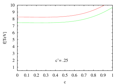
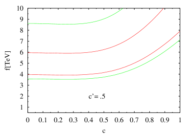
Figure 1: 90% and 50% CL exclusion contours in the plane $f$-$c$ for two values of the cosine of the other mixing angle $c^{\prime}$ in the littlest Higgs model. The value of the triplet vev $v^{\prime}$ is chosen using $v^{\prime}/v=v/(4f)$. Other choices of $v^{\prime}$ do not change much the above conclusions. The allowed region lies above the bands for the left figure and inside the bands for the right one (90% CL the narrowest (in red) and 50% CL the largest (in green)).

Our result for the corrections to the $\epsilon_{i}$ parameters to the order $v^{2}/f^{2}$ is given by:

$$\epsilon_{1} = -\frac{v^{2}}{f^{2}}\left(\frac{5}{4}(c^{\prime 2}-s^{\prime 2})^{2}+\frac{4}{5}(c^{\prime 2}-s^{\prime 2})(3c^{\prime 2}-2s^{\prime 2})+2c^{4}\right)+4\frac{v^{\prime 2}}{v^{2}}$$ (14)

$$\epsilon_{2} = -2c^{4}\frac{v^{2}}{f^{2}}$$ (15)

$$\epsilon_{3} = -\frac{v^{2}}{f^{2}}\left(\frac{1}{2}c^{2}(c^{2}-s^{2})+\frac{2}{5}(c^{\prime 2}-s^{\prime 2})(3c^{\prime 2}-2s^{\prime 2})\frac{c_{\theta}^{2}}{s_{\theta}^{2}}\right)$$ (16)

Notice that the corrections, as they should, depend only on the parameters $c$, $c^{\prime}$, $v/f$ and $v^{\prime}/v$.

The model is strongly constrained by the precision electroweak data as can be seen in figure 1. For large values of $v/f$ the allowed regions are very small, whereas for small values practically the entire parameter space is excluded. For large values of $v/f$ this is mainly due to the fact that this model exhibits no custodial symmetry and that it is therefore difficult to satisfy the experimental constraint on $\epsilon_{1}$ without fine tuning of the parameters. For small values of $v/f$ we approach the SM limit which itself is not in agreement with the values for the $\epsilon$-parameters.

2.2 Little Higgs with custodial $SU(2)$

We now examine a “little Higgs” model which has an approximate custodial $SU(2)$ symmetry $\!{}^{{\bf?}}$. The model is based on a $SO(9)/[SO(5)\times SO(4)]$ coset space, with $SU(2)_{L}\times SU(2)_{R}\times SU(2)\times U(1)$ subgroup of $SO(9)$ gauged.

One starts with an orthogonal symmetric nine by nine matrix, representing a nonlinear sigma model field $\Sigma$ which transforms under an $SO(9)$ rotation by $\Sigma\to V\Sigma V^{T}$. To break the $SO(4)$’s to the diagonal, one can take $\Sigma$’s vev to be

$$\langle\Sigma\rangle=\left(\begin{array}[]{ccc}0&0&{\hbox to0.0pt{1\hss}\hskip 1.6pt\hbox{1}}_{4}\\ 0&1&0\\ {\hbox to0.0pt{1\hss}\hskip 1.6pt\hbox{1}}_{4}&0&0\end{array}\right)$$ (20)

breaking the $SO(9)$ global symmetry down to an $SO(5)\times SO(4)$ subgroup. This coset space has $20=(36-10-6)$ light scalars. Of these 20 scalars, 6 will be eaten in the higgsing of the gauge groups down to $SU(2)_{W}\times U(1)_{Y}$. The remaining 14 scalars are : a single higgs doublet $h$, an electroweak singlet $\phi^{0}$, and three triplets $\phi^{ab}$ which transform under the $SU(2)_{L}\times SU(2)_{R}$ diagonal symmetry as

$$h:(\mathbf{2}_{L},\mathbf{2}_{R})\hskip 36.135pt\phi^{0}:(\mathbf{1}_{L},\mathbf{1}_{R})\hskip 36.135pt\phi^{ab}:(\mathbf{3}_{L},\mathbf{3}_{R}).$$ (21)

These fields can be written

$$\Sigma=e^{i\Pi/f}\langle\Sigma\rangle e^{i\Pi^{T}/f}=e^{2i\Pi/f}\langle\Sigma\rangle$$ (22)

with

$$\Pi=\frac{-i}{4}\left(\begin{array}[]{ccc}0_{4\times 4}&\sqrt{2}\vec{h}&-\Phi\\ -\sqrt{2}\vec{h}^{T}&0_{1\times 1}&\sqrt{2}\vec{h}^{T}\\ \Phi&-\sqrt{2}\vec{h}&0_{4\times 4}\end{array}\right)$$ (26)

where the Higgs doublet $\vec{h}$ is written as an $SO(4)$ vector; the singlet and triplets are in the symmetric four by four matrix $\Phi$

$$\Phi=\phi^{0}+4\phi^{ab}\>T^{l\,a}T^{r\,b}\,,$$ (27)

and the would-be Goldstone bosons that are eaten in the higgsing to $SU(2)_{W}\times U(1)_{Y}$ are set to zero in $\Pi$. The global symmetries protect the higgs doublet from one-loop quadratic divergent contributions to its mass. However, the singlet and triplets are not protected, and are therefore heavy, in the region of the TeV scale. The theory contains the minimal top sector with two extra coloured quark doublets and their charge conjugates. Further details and formulas can be found in $\!{}^{{\bf?}}$.

The kinetic energy for the pseudo-Goldstone bosons is

$${\cal L}_{kin}=\frac{f^{2}}{4}{\rm Tr}\left[D_{\mu}\Sigma D^{\mu}\Sigma\right]$$ (28)

and the covariant derivative is

$$D_{\mu}\Sigma=\partial_{\mu}\Sigma+i\left[A_{\mu},\Sigma\right]$$ (29)

where the gauge boson matrix $A_{\mu}$ is defined as

$$A\equiv g_{L}W^{la}_{SO(4)}\tau^{l\,a}+g_{R}W^{ra}_{SO(4)}\tau^{r\,a}+g_{2}W^{la}\eta^{l\,a}+g_{1}W^{r3}\eta^{r\,3}.$$ (30)

The $\tau^{a}$ and $\eta^{a}$ are the generators of two SO(4) subgroups of SO(9). For details see Ref. $\!{}^{{\bf?}}$.

The vector bosons can be diagonalized with the following transformations:

$$B = c^{\prime}W^{r3}-s^{\prime}W_{SO(4)}^{r3}\hskip 36.135ptB^{\prime}=W^{\prime}{}^{\,r3}=s^{\prime}W^{r3}+c^{\prime}W_{SO(4)}^{r3}$$ (31)

$$W^{a} = cW^{la}+sW_{SO(4)}^{la}\hskip 36.135ptW^{\prime}{}^{a}=W^{\prime}{}^{\,la}=-sW^{la}+cW_{SO(4)}^{la}$$ (32)

where the cosines and the sines of the mixing angles can be written in terms of the couplings

$$c^{\prime} = g^{\prime}/g_{1}\hskip 36.135pts^{\prime}=g^{\prime}/g_{R}$$

$$c = g/g_{2}\hskip 36.135pts=g/g_{L}.$$ (33)

Again $g$ and $g^{\prime}$ are defined in terms of $g_{1}$, $g_{R}$ and $g_{2}$, $g_{L}$ respectively, as in equation (6).

We now proceed in exactly the same way as in the previous section and look first at the modifications to $G_{F}$. The expression for $G_{F}$ in terms of the model parameters is

$$\frac{G_{F}}{\sqrt{2}}=\frac{\alpha\pi(g^{2}+g^{\prime 2})^{2}}{2g^{2}g^{\prime 2}}\left(1+\frac{v^{2}}{f^{2}}\frac{s^{2}(c^{2}-s^{2})-s^{4}}{2}\right)~{},$$ (34)

The masses of $Z$- and $W$-bosons are given by

$$m_{Z}^{2}=(g^{2}+g^{\prime 2})\frac{v^{2}+4v^{\prime 2}}{4}$$ (35)

$$m_{W}^{2}=\frac{g^{2}v^{2}}{4}\left(1+2\frac{v^{\prime 2}+{\tilde{v}}^{\prime 2}}{v^{2}}\right)~{}.$$ (36)

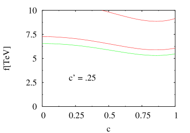
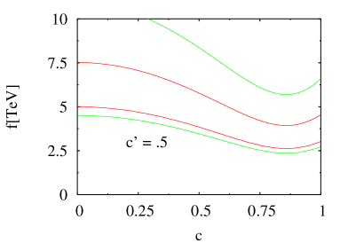
Figure 2: Exclusion plots in the plane $f$-$c$ for two values of the cosine of the other mixing angle $c^{\prime}$ in the $SO(9)/[SO(5)\times SO(4)]$ model. In the plot with $c^{\prime}=0.25$ the value of the triplet vevs is chosen $v^{\prime 2}/v^{2}=v^{2}/(4f^{2})$ and ${\tilde{v}}^{\prime 2}/v^{2}=v^{2}/(2f^{2})$, while in the one with $c^{\prime}=0.5$ the triplet vevs are $v^{\prime 2}/v^{2}={\tilde{v}}^{\prime 2}/v^{2}=v^{2}/(4f^{2})$. The allowed region lies inside the bands (90% CL the narrowest (in red) and 50% CL the largest (in green)).

The $Z$ and $W$-mass only receive corrections from the triplet vevs ($v^{\prime}$ is the $Y=1$ and ${\tilde{v}}^{\prime}$ the $Y=0$ triplet vev). This is a consequence of the approximate custodial symmetry of the model.

The corrections to the $\epsilon$ parameters to the order $v^{2}/f^{2}$ are

$$\epsilon_{1} = \frac{v^{2}}{4f^{2}}\left[4s^{\prime\,2}\left(c^{\prime\,2}-s^{\prime\,2}\right)+2c^{2}s^{2}-s^{4}\right]+2\frac{{\tilde{v}}^{\prime 2}-v^{\prime 2}}{v^{2}}$$ (37)

$$\epsilon_{2} = \frac{v^{2}}{4c_{2\theta}\,f^{2}}\Big{[}4s^{\prime\,2}\left(c^{\prime\,2}-s^{\prime\,2}\right)c_{\theta}^{2}c_{2\theta}+2s^{2}\left(c^{2}-s^{2}\right)\left(c^{4}_{\theta}-3c^{2}_{\theta}s^{2}_{\theta}+2c^{2}_{\theta}-s^{2}_{\theta}\right)$$ (38)

$$+ s^{4}(c^{4}_{\theta}+s^{4}_{\theta})\Big{]}$$

$$\epsilon_{3} = \frac{v^{2}}{2s^{2}_{\theta}\,f^{2}}\left[s^{2}\left(c^{2}-s^{2}\right)\left(-c_{2\theta}+2s_{\theta}^{2}c_{\theta}^{2}\right)-s^{4}c^{2}_{\theta}s^{2}_{\theta}\right]+\frac{2c^{2}_{\theta}}{v^{2}s^{2}_{\theta}}\left(v^{\prime 2}-{\tilde{v}}^{\prime 2}\right)~{},$$ (39)

where we have used the definition of $s_{\theta}$ and $c_{\theta}$ via Eq. 11. The results of the analysis are shown in Fig. 2 for a choiche of the model parameters. The allowed region lies inside the bands. As can be inferred from the expression of the $\epsilon$’s, a large value of difference of the triplet vevs spoil the custodial symmetry. Note however that one can argue that the two different triplet vevs should be similar in size and at least partially compensate their effects since the only violations come from the $U(1)$ coupling which has to be smaller than the $SU(2)_{R}$ coupling $\!{}^{{\bf?}}$. Therefore the custodial violation is not a problem for the custodial model. A precise evaluation of this effect is not possible in the effective theory since there are unknown order one factors in the radiatively generated potential.

3 Low energy precision data

Precision experiments at low energy allow a precise determination of the $g-2$ of the muon and of the weak charge of cesium atoms. Concerning the $g-2$ of the muon, the contributions of the additional heavy particles are completely negligible and the dominant contributions arise from the corrections to the light $Z$ and $W$ couplings. On the contrary the measure of the weak charge of cesium atoms, gives constraints on the little Higgs models, even if weaker that those at LEP energies. Parity violation in atoms is due to the electron-quark effective Lagrangian

$$\mathcal{L}_{\mathit{eff}}=\frac{G_{F}}{\sqrt{2}}(\bar{e}\gamma_{\mu}\gamma_{5}e)(C_{1u}\bar{u}\gamma^{\mu}u+C_{1d}\bar{d}\gamma^{\mu}d)~{}.$$ (40)

The experimentally measured quantity is the so-called “weak charge” defined as

$$Q_{W}=-2\left(C_{1u}(2Z+N)+C_{1d}(Z+2N)\right)~{},$$ (41)

where Z, N are the number of protons and neutrons of the atom, respectively.

The effective Lagrangian, Eq. 40, can be derived from the interaction of $Z,Z_{H},$ and $A_{H}$ with the fermions by integrating out the heavy degrees of freedom. The difference of the weak charge of Cs is shown in Fig. 3 for the model with approximate custodial symmetry. As experimental input for our analysis we have again used $m_{Z},G_{F},$ and $\alpha$. In order to discuss the weak charge result, let’s consider the value $\delta Q_{W}(Cs)=1$ which is close to the present experimental central value. It is clear from Fig. 3 that the value of the high scale $f$ should be in the range of few TeV in order to obtain the measured deviation. The allowed scale is slightly lower in the custodial model with respect to the non-custodial one as the custodial model is closer to the standard model in its predictions. When the scale $f$ is too large the new physics effects become negligible. The scale $f$ in the few TeV range is consistent with what is expected on the model-building side and from the LEP data for little Higgs model. Obviously this result should be taken only as a first indication as the error on $\delta Q_{W}(Cs)$ is large.

Figure 3: Corrections to the weak charge of cesium atoms as a function of $c$ and $c^{\prime}$ in the little Higgs model with approximate custodial symmetry.

4 Conclusions

The analysis of precision electroweak data gives rather stringent limits on the littlest Higgs model. This is mainly due to the difficulty of the model to accommodate for the experimental results of the $\rho$ parameter. In the model where custodial symmetry is approximately fulfilled, less fine tuning than in the littlest Higgs model is needed in order to satisfy the experimental constraints. Thus custodial symmetry seems to be an essential ingredient for realistic little Higgs models. Constraints from low energy precision data., i.e., $g-2$ of the muon and the atomic ”weak charge” of the cesium, do not change the above conclusions. For $g-2$ of the muon the corrections are simply too small to impose any new constraints on the model parameters. The actual state of precision for the weak charge does not allow for establishing new constraints either, even if the corrections are not negligible.

References

References

- [1] N. Arkani-Hamed, A. G. Cohen and H. Georgi, Phys. Lett. B 513, 232 (2001) [arXiv:hep-ph/0105239]; N. Arkani-Hamed, A. G. Cohen, T. Gregoire and J. G. Wacker, JHEP 08, 020 (2002) [arXiv:hep-ph/0202089]; N. Arkani-Hamed, A. G. Cohen, E. Katz, A. E. Nelson, T. Gregoire and J. G. Wacker; JHEP 08, 021 (2002) [arXiv:hep-ph/0206020]. N. Arkani-Hamed, A. G. Cohen, E. Katz and A. E. Nelson, JHEP 07, 034 (2002) [arXiv:hep-ph/0206021]; I. Low, W. Skiba and D. Smith, Phys. Rev. D 66, 072001 (2002) [arXiv:hep-ph/0207243]; for a review, see, e.g., M. Schmaltz, Nucl. Phys. Proc. Suppl. 117, 40 (2003) [arXiv:hep-ph/0210415].
- [2] S. Dimopoulos and J. Preskill, Nucl. Phys. B 199, 206 (1982); D. B. Kaplan and H. Georgi, Phys. Lett. 136B, 183 (1984); D. B. Kaplan, H. Georgi and S. Dimopoulos, Phys. Lett. 136B, 187 (1984); H. Georgi and D. B. Kaplan, Phys. Lett. 145B, 216 (1984); H. Georgi, D. B. Kaplan and P. Galison, Phys. Lett. 143B, 152 (1984); M. J. Dugan, H. Georgi and D. B. Kaplan, Nucl. Phys. B 254, 299 (1985); T. Banks, Nucl. Phys. B 243, 125 (1984).
- [3] C. Csaki, J. Hubisz, G. D. Kribs, P. Meade and J. Terning, Phys. Rev. D 67, 115002 (2003) [arXiv:hep-ph/0211124] and Phys. Rev. D 68, 035009 (2003) [arXiv:hep-ph/0303236]; J. L. Hewett, F. J. Petriello and T. G. Rizzo, JHEP 0310, 062 (2003) [arXiv:hep-ph/0211218]; G. Burdman, M. Perelstein and A. Pierce, Phys. Rev. Lett. 90 (2003) 241802 [arXiv:hep-ph/0212228]; T. Gregoire, D. R. Smith and J. G. Wacker, arXiv:hep-ph/0305275; M. Perelstein, M. E. Peskin and A. Pierce, Phys. Rev. D 69 (2004) 075002 [arXiv:hep-ph/0310039].
- [4] G. Altarelli and R. Barbieri, Phys. Lett. B 253, 161 (1991); G. Altarelli, R. Barbieri and S. Jadach, Nucl. Phys. B 369, 3 (1992) [Erratum-ibid. B 376, 444 (1992)].
- [5] B. Grinstein and M. B. Wise, Phys. Lett. B 265 (1991) 326; R. Barbieri, A. Pomarol, R. Rattazzi and A. Strumia, arXiv:hep-ph/0405040.
- [6] R. Casalbuoni, A. Deandrea and M. Oertel, JHEP 0402 (2004) 032 [arXiv:hep-ph/0311038]; M. C. Chen and S. Dawson, arXiv:hep-ph/0311032; W. Kilian and J. Reuter, arXiv:hep-ph/0311095.
- [7] S. Chang and H. J. He, Phys. Lett. B 586 (2004) 95 [arXiv:hep-ph/0311177].
- [8] T. Han, H. E. Logan, B. McElrath and L. T. Wang, Phys. Rev. D 67, 095004 (2003) [arXiv:hep-ph/0301040].
- [9] L. Anichini, R. Casalbuoni and S. De Curtis, Phys. Lett. B 348, 521 (1995) [arXiv:hep-ph/9410377].
- [10] S. Chang and J. G. Wacker, Phys. Rev. D 69 (2004) 035002 [arXiv:hep-ph/0303001]; S. Chang, JHEP 0312 (2003) 057 [arXiv:hep-ph/0306034].