The Littlest Higgs boson at a photon collider

Abstract

We calculate the corrections to the partial widths of the light Higgs boson in the Littlest Higgs model due to effects of the TeV-scale physics. We focus on the loop-induced Higgs coupling to photon pairs, which is especially sensitive to the effects of new particles running in the loop. This coupling can be probed with high precision at a photon collider in the process $\gamma\gamma\to H\to b\bar{b}$ for a light Higgs boson with mass 115 GeV $\leq M_{H}\lesssim 140$ GeV. Using future LHC measurements of the parameters of the Littlest Higgs model, one can calculate a prediction for this process, which will serve as a test of the model and as a probe for a strongly-coupled UV completion at the 10 TeV scale. We outline the prospects for measuring these parameters with sufficient precision to match the expected experimental uncertainty on $\gamma\gamma\to H\to b\bar{b}$.

I Introduction

Understanding the mechanism of electroweak symmetry breaking (EWSB) is the central goal of particle physics today. A full understanding of EWSB will include a solution to the hierarchy or naturalness problem – that is, why the weak scale is so much lower than the Planck scale. Whatever is responsible for EWSB and its hierarchy, it must manifest experimentally at or below the TeV energy scale.

Our first glimpse at the EWSB scale came from the electroweak precision data from the CERN LEP collider, which is sensitive to the Higgs boson mass in the Standard Model (SM) via radiative corrections. This electroweak precision data points to the existence of a light Higgs boson in the SM, with mass below roughly 200 GeV LEPEWWG .

The TeV scale is currently being probed at the Fermilab Tevatron and will soon be thoroughly explored at the CERN Large Hadron Collider (LHC). Further into the future, a linear $e^{+}e^{-}$ collider will offer an excellent opportunity to study the dynamics of the new physics with uniquely high precision. The wealth of data on TeV scale physics promised by this experimental program has driven model-building on the theoretical side.

A wide variety of models have been introduced over the past three decades to address EWSB and the hierarchy problem: supersymmetry, extra dimensions, strong dynamics leading to a composite Higgs boson, and the recent “little Higgs” models Littlest ; LHModels in which the Higgs is a pseudo-Goldstone boson. In this paper we consider the last possibility. For concreteness, we choose a particular model framework, the “Littlest Higgs” Littlest , for our calculations.

In the little Higgs models, the SM Higgs doublet appears as a pseudo-Goldstone boson of an approximate global symmetry that is spontaneously broken at the TeV scale. The models are constructed as nonlinear sigma models, which become strongly coupled (and thus break down) no more than one loop factor above the spontaneous symmetry breaking scale. In fact, in many models unitarity violation in longitudinal gauge boson scattering appears to occur only a factor of a few above the spontaneous symmetry breaking scale, due to the large multiplicity of Goldstone bosons Hong-Jian . Thus the little Higgs models require an ultraviolet (UV) completion at roughly the 10 TeV scale. The first UV completions of little Higgs models have been constructed in Refs. UVcompletion ; turtles .

The explicit breaking of the global symmetry, by gauge, Yukawa and scalar interactions, gives the Higgs a mass and non-derivative interactions, as required of the SM Higgs doublet. The little Higgs models are constructed in such a way that no single interaction breaks all of the symmetry forbidding a mass term for the SM Higgs doublet. This guarantees the cancellation of the one-loop quadratically divergent radiative corrections to the Higgs boson mass. Quadratic sensitivity of the Higgs mass to the cutoff scale then arises only at the two-loop level, so that a Higgs mass at the 100 GeV scale, two loop factors below the 10 TeV cutoff, is natural.

A light Higgs boson is the central feature of the little Higgs models. In the Littlest Higgs model, the couplings of the Higgs boson to SM particles receive corrections due to the new TeV-scale particles LHpheno ; LHloop ; Kilian ; Deandrea . These corrections are suppressed by the square of the ratio of the electroweak scale to the TeV scale, and are thus parametrically at the level of a few percent. Percent-level measurements of Higgs couplings are expected to be possible at a future linear $e^{+}e^{-}$ collider and its photon collider extension.

Corrections to the Higgs couplings can also be induced by the UV completion at 10 TeV. For example, the loop-induced Higgs coupling to photon pairs receives corrections from new heavy particles running in the loop. If the UV completion is weakly coupled, these corrections should naively be suppressed by the square of the ratio of the electroweak scale to the 10 TeV scale, and thus be too small to detect with the expected experimental capabilities. However, if the UV completion is strongly coupled, the strong-coupling enhancement counteracts the suppression from the high mass scale, leading to corrections naively of the same order as those from the TeV scale physics. To reiterate, if the UV completion is weakly coupled, we expect the corrections to the Higgs couplings to be accurately predicted by the TeV-scale theory alone. However, if the UV completion is strongly coupled, we expect the Higgs couplings to receive corrections from the UV completion at the same level as the corrections from the TeV-scale theory.

The parameters of the Littlest Higgs model can be measured at the LHC and then used to calculate predictions for the corrections to the Higgs couplings due to the TeV-scale physics. Comparing these predictions to high-precision Higgs coupling measurements will serve as a test of the model, as well as a probe for a strongly-coupled UV completion. In this paper, we focus on the process $\gamma\gamma\to H\to b\bar{b}$, the rate for which will be measured with high precision at a future photon collider.

This paper is organized as follows. We begin in Sec. II with a brief review of the experimental prospects and a general discussion of the bounds that can be put on the dimension-six operator that generates a non-SM Higgs coupling to photon pairs. In Sec. III we outline the Littlest Higgs model Littlest , following the notation of Refs. LHpheno ; LHloop . In Sec. IV we calculate the corrections to the Higgs couplings due to the TeV-scale new physics in the Littlest Higgs model, focusing on the correction to $\gamma\gamma\to H\to b\bar{b}$.

In order to make predictions for the Higgs couplings, the TeV-scale model parameters must be measured. In Sec. V we estimate the precision with which the parameters of the TeV-scale theory must be measured at the LHC in order to give theoretical predictions that match the precision of the photon collider measurement, and discuss the prospects for doing so. In Sec. VI we address the additional sources of experimental and theoretical uncertainty that affect our probe of the model. Section VII is reserved for our conclusions. Formulas for the coupling correction factors are collected in an Appendix.

II Higgs production at a photon collider

II.1 Experimental considerations

If the Higgs boson is sufficiently SM-like, its discovery is guaranteed at the LHC LHCTDRs . Its mass will be measured with high precision LHCTDRs , and in addition, LHC measurements of Higgs event rates in various signal channels allow for the extraction of certain combinations of Higgs partial widths at the $10-30\%$ level LHCHiggsMeas . A future $e^{+}e^{-}$ linear collider will measure the production cross section of a light Higgs boson in Higgsstrahlung or $WW$ fusion with percent-level precision, as well as the important branching fractions with few-percent precision LCs ; TESLATDR . A photon collider, which can be constructed from a linear $e^{+}e^{-}$ or $e^{-}e^{-}$ collider through Compton backscattering of lasers from the $e^{\pm}$ beams, can also measure rates for Higgs production (in two-photon fusion) and decay into certain final states with few-percent level precision ggAsner ; LeptonPhoton ; Ohgaki ; AGG ; Jikia ; Krawczyk1 ; Krawczyk2 ; Rosca .

In this paper we focus on the Higgs coupling measurements that can be made at a photon collider. Experimental studies of the expected precisions with which the rates for $\gamma\gamma\to H\to X$ can be measured have been done for various photon collider designs (NLC, TESLA, JLC, and CLICHE); their results are summarized in Table 1.

Study		$M_{H}$	$b\bar{b}$	$WW^{*}$	$\gamma\gamma$
CLICHE	ggAsner ; LeptonPhoton	115 GeV	2%	5%	22%
JLC	Ohgaki	120 GeV	7.6%	–	–
NLC	AGG	120 GeV	2.9%	–	–
		160 GeV	10%	–	–
TESLA	Jikia ; Krawczyk1 ; Krawczyk2 ; Rosca	120 GeV	1.7–2%	–	–
	Krawczyk2	130 GeV	1.8%	–	–
		140 GeV	2.1%	–	–
		150 GeV	3.0%	–	–
	Jikia ; Krawczyk2	160 GeV	7.1–10%	–	–

Table 1: Expected experimental precision of the rate measurement of $\gamma\gamma\to H\to X$. Dashes indicate that the corresponding study has not been done. Not included are studies of Higgs boson decays to $WW$, $ZZ$ KrawczykHighM and $t\bar{t}$ Asakawa for $M_{H}\geq 200$ GeV.

All the studies assume roughly one year’s running at design luminosity. The variations in results between different studies at the same Higgs mass are believed to be due mostly to the different photon beam spectra and luminosities at the different machines. In all cases $\sqrt{s_{ee}}$ and the electron and laser polarizations have been optimized for maximum Higgs production.

From Table 1 we take away two lessons: (1) the rate for $\gamma\gamma\to H\to b\bar{b}$ can be measured to about 2% for a SM-like Higgs boson with 115 GeV $\leq M_{H}\lesssim 140$ GeV, and (2) this precision is better than will be obtained for any other Higgs decay mode for a Higgs boson in this mass range.

II.2 Probing the $\gamma\gamma H$ coupling

In the SM, the $\gamma\gamma H$ coupling arises from the loop-induced dimension-6 operator

$$\mathcal{L}=\frac{C}{\Lambda^{2}}h^{\dagger}hF^{\mu\nu}F_{\mu\nu},$$ (1)

where $h$ is the Higgs doublet, $F^{\mu\nu}$ is the electromagnetic field strength tensor, $\Lambda$ is the mass scale that characterizes the interaction, and $C$ is a dimensionless coefficient. This operator leads to the Higgs boson partial width into photon pairs,

$$\Gamma_{\gamma}=\frac{C^{2}v^{2}M_{H}^{3}}{2\pi\Lambda^{4}},$$ (2)

where $v=246$ GeV is the SM Higgs vacuum expectation value (vev) and $M_{H}$ is the physical Higgs mass.

Taking, e.g., $M_{H}=115$ GeV, we compute the partial width $\Gamma_{\gamma}$ using HDECAY HDECAY to be

$$\Gamma_{\gamma}=6.65\times 10^{-6}\ {\rm GeV}.$$ (3)

This leads to the following estimate for the scale $\Lambda$ for the SM loops that give rise to the $\gamma\gamma H$ coupling, for various choices of $C$:

$$\Lambda_{\rm SM}=\left\{\begin{array}[]{rl}6.8\ {\rm TeV}&C=1\\ 550\ {\rm GeV}&C=1/16\pi^{2}\\ 170\ {\rm GeV}&C=e^{2}/16\pi^{2}.\end{array}\right.$$ (4)

The SM coupling is generated primarily by $W$ boson and top quark loops, with a characteristic energy scale around the weak scale. This shows the importance of the loop suppression and electromagnetic coupling suppression of the operator in Eq. (1).

If new physics beyond the SM contributes to the $\gamma\gamma H$ coupling, we can parameterize its effect in Eq. (1) through

$$\frac{C}{\Lambda^{2}}\to\frac{C_{\rm SM}}{\Lambda^{2}_{\rm SM}}+\frac{C_{\rm new}}{\Lambda^{2}_{\rm new}}.$$ (5)

With the assumption that $C_{\rm SM}/\Lambda_{\rm SM}^{2}\gg C_{\rm new}/\Lambda_{\rm new}^{2}$, we can write the new physics correction relative to the SM partial width as

$$\frac{\delta\Gamma_{\gamma}}{\Gamma_{\gamma}}\simeq 2\left|\frac{C_{\rm new}}{C_{\rm SM}}\right|\frac{\Lambda^{2}_{\rm SM}}{\Lambda^{2}_{\rm new}}.$$ (6)

As in Eq. (4), the scale $\Lambda_{\rm new}$ that can be probed with a measurement of $\Gamma_{\gamma}$ depends on the assumption for $C_{\rm new}$. We consider two possibilities: weakly-coupled loops, $C_{\rm new}=e^{2}/16\pi^{2}$, and strongly-coupled loops, $C_{\rm new}=1$. Assuming that $\Gamma_{\gamma}$ can be measured with 2% precision, we find sensitivity to new physics scales at various confidence levels as given in Table 2.

	$\Lambda_{\rm new}$
Confidence level	($C_{\rm new}=e^{2}/16\pi^{2}$)	($C_{\rm new}=1$)
$1\sigma$	1.7 TeV	68 TeV
$2\sigma$	1.2 TeV	48 TeV
$5\sigma$	0.74 TeV	31 TeV

Table 2: Sensitivity to the new physics scale $\Lambda_{\rm new}$ from a 2% measurement of $\Gamma_{\gamma}$ at various confidence levels, assuming the new physics is weakly coupled ($C_{\rm new}=e^{2}/16\pi^{2}$) or strongly coupled ($C_{\rm new}=1$). $\Lambda_{\rm SM}$ was computed for a 115 GeV SM Higgs boson using HDECAY HDECAY .

We find that the reach of this measurement for weakly-coupled new physics is at the 1 TeV scale, while for strongly-coupled new physics it is at the few tens of TeV scale.

III The Littlest Higgs model

In this section we outline the Littlest Higgs model Littlest and define the parameters relevant for our analysis, following the notation of Refs. LHpheno ; LHloop .

The Littlest Higgs model consists of a nonlinear sigma model with a global SU(5) symmetry which is broken down to SO(5) by a vacuum condensate $f\sim$ TeV. A subgroup SU(2)${}_{1}\times$SU(2)${}_{2}\times$U(1)${}_{1}\times$U(1)₂ of the global SU(5) is gauged, with gauge couplings $g_{1}$, $g_{2}$, $g_{1}^{\prime}$ and $g_{2}^{\prime}$, respectively. The breaking of the global SU(5) down to SO(5) by the condensate $f$ simultaneously breaks the gauge group down to its diagonal SU(2)$\times$U(1) subgroup, which is identified as the SM electroweak gauge group. The breaking of the global symmetry gives rise to 14 Goldstone bosons, four of which are eaten by the broken gauge generators, leading to four vector bosons with masses of order $f$: an SU(2) triplet, $Z_{H}$ and $W_{H}^{\pm}$, and a U(1) boson $A_{H}$.

Besides the condensate $f$, the heavy gauge boson sector is parameterized in terms of two mixing angles,

$$0<c\equiv\cos\theta=\frac{g_{1}}{\sqrt{g_{1}^{2}+g_{2}^{2}}}<1,\qquad\qquad 0<c^{\prime}\equiv\cos\theta^{\prime}=\frac{g_{1}^{\prime}}{\sqrt{g_{1}^{\prime 2}+g_{2}^{\prime 2}}}<1.$$ (7)

We also define $s\equiv\sqrt{1-c^{2}}$ and $s^{\prime}\equiv\sqrt{1-c^{\prime 2}}$. The TeV-scale gauge boson masses are given to leading order in $v^{2}/f^{2}$ in terms of these parameters by

$$M_{Z_{H}}=M_{W_{H}}=\frac{gf}{2sc},\qquad\qquad M_{A_{H}}=\frac{g^{\prime}f}{2\sqrt{5}s^{\prime}c^{\prime}}.$$ (8)

The parameters $c$ and $c^{\prime}$ also control the couplings of the heavy gauge bosons to fermions.

An alternate version of the model, which we will also consider, starts with only SU(2)${}_{1}\times$SU(2)${}_{2}\times$U(1)_Y gauged; this model contains no $A_{H}$ boson. Since the $A_{H}$ boson tends to cause significant custodial isospin breaking and corrections to four-fermion neutral current interactions, this alternate version of the model is preferred by the electroweak precision data GrahamEW1 ; JoAnneEW ; GrahamEW2 . Since the $A_{H}$ is typically also quite light, this version is also preferred by the direct exclusion bounds from the Tevatron JoAnneEW ; Park .

The ten remaining uneaten Goldstone bosons transform under the SM gauge group as a doublet $h$ (identified as the SM Higgs doublet) and a triplet $\phi$. The components $\Phi^{++}$, $\Phi^{+}$, $\Phi^{0}$ (scalar) and $\Phi^{P}$ (neutral pseudoscalar) of the triplet get a mass, to leading order in $v^{2}/f^{2}$, of

$$M_{\Phi}=\frac{\sqrt{2}M_{H}f}{v\sqrt{1-x^{2}}},$$ (9)

where $x$ is a free parameter of the Higgs sector proportional to the triplet vev $v^{\prime}$ and defined as

$$0\leq x=\frac{4fv^{\prime}}{v^{2}}<1.$$ (10)

The constraint $x<1$ is required to obtain the correct electroweak symmetry breaking vacuum and avoid giving a TeV-scale vev to the scalar triplet (see Ref. LHpheno for further details).

Finally, the top quark sector is modified by the addition of a heavy top-like quark $T$. The top sector is parameterized by

$$0<c_{t}=\frac{\lambda_{1}}{\sqrt{\lambda_{1}^{2}+\lambda_{2}^{2}}}<1,$$ (11)

where the dimensionless couplings $\lambda_{1,2}$ are defined according to the normalization given in Ref. LHpheno . Together with $f$, this parameter controls the $T$ mass (we also define $s_{t}\equiv\sqrt{1-c_{t}^{2}}$),

$$M_{T}=\frac{m_{t}f}{vs_{t}c_{t}}.$$ (12)

The parameter $c_{t}$ also controls the mixing between $t$ and $T$ at order $v^{2}/f^{2}$, which generates a $TbW$ coupling leading to single $T$ production through $bW$ fusion at hadron colliders LHpheno ; Peskin .

IV Corrections to Higgs observables

In any theory beyond the SM, corrections to SM observables must be calculated relative to the SM predictions for a given set of SM electroweak inputs. These electroweak inputs are usually taken to be the Fermi constant $G_{F}$ defined in muon decay, the $Z$ mass $M_{Z}$, and the electromagnetic fine structure constant $\alpha$. Thus, a calculation of corrections to, e.g., Higgs couplings due to new physics must necessarily involve a calculation of the corrections to the SM electroweak input parameters due to the same new physics.

In the Littlest Higgs model, it is most straightforward to calculate the corrections to the Higgs couplings in terms of the SM Higgs vev $v=246$ GeV. To obtain useful predictions of the couplings, this must be related to the Fermi constant in the Littlest Higgs model according to $v^{-2}=\sqrt{2}G_{F}y^{2}_{G_{F}}$, where $y^{2}_{G_{F}}=1+\mathcal{O}(v^{2}/f^{2})$ is a correction factor given in the Appendix.

IV.1 Higgs partial widths

In this section we present the formulas for the corrections to the Higgs partial widths to SM particles. We write the partial widths $\Gamma_{i}$ in the Littlest Higgs model normalized to the corresponding SM partial width, $\Gamma_{i}^{\rm SM}$. The partial widths are written in terms of correction factors $y_{i}$, which are collected in the Appendix. For the SM electroweak inputs we take the parameters $G_{F}$, $M_{Z}$ and $\alpha$.

The corrections to the loop-induced partial widths of the Higgs boson into photon pairs and gluon pairs were computed in the Littlest Higgs model in Ref. LHloop ; we list them in the Appendix for completeness.

The corrections to the tree-level couplings of the Higgs boson in the Littlest Higgs model can be derived to order $v^{2}/f^{2}$ from the couplings given in Ref. LHpheno . The partial widths of the Higgs boson into $Z$ boson pairs ($\Gamma_{Z}$), top quark pairs ($\Gamma_{t}$), and pairs of other fermions ($\Gamma_{f}$) normalized to their SM values are given by

$$\Gamma_{Z}/\Gamma_{Z}^{\rm SM}=y^{2}_{G_{F}}y^{2}_{Z},\qquad\qquad\Gamma_{t}/\Gamma_{t}^{\rm SM}=y^{2}_{G_{F}}y^{2}_{t},\qquad\qquad\Gamma_{f}/\Gamma_{f}^{\rm SM}=y^{2}_{G_{F}}y^{2}_{f}.$$ (13)

The correction to the partial width for the Higgs decay to $W$ bosons is a little subtle when $G_{F}$, $M_{Z}$ and $\alpha$ are used as inputs because the relation between these inputs and the physical $W$ boson mass receives corrections from the Littlest Higgs model. The partial width of $H\to WW^{(*)}$ depends on the $W$ mass in the kinematics, especially in the intermediate Higgs mass range, $115\ {\rm GeV}\lesssim M_{H}\lesssim 2M_{W}$. To deal with this, we follow the same approach taken by the program HDECAY HDECAY for the Minimal Supersymmetric Standard Model (MSSM), which is to define the $H\to WW^{(*)}$ partial width in the MSSM in terms of the SM partial width simply by scaling by the ratio of the $WWH$ couplings-squared in the two models, ignoring the shift in the kinematic $W$ mass. Thus, we calculate only the correction to the coupling-squared in the Littlest Higgs model, and do not worry about the shift due to the $W$ mass correction in the kinematics. We find,

$$\Gamma_{W}/\Gamma_{W}^{\rm SM}=y^{2}_{G_{F}}y^{2}_{W}\frac{y^{4}_{M_{W}}}{y^{4}_{M_{Z}}}y^{4}_{c_{W}}.$$ (14)

The corrections to the Higgs couplings involved in $\Gamma_{Z}/\Gamma_{Z}^{\rm SM}$, $\Gamma_{f}/\Gamma_{f}^{\rm SM}$, $\Gamma_{t}/\Gamma_{t}^{\rm SM}$, and $\Gamma_{W}/\Gamma_{W}^{\rm SM}$ in the Littlest Higgs model were derived previously in Ref. Kilian by integrating out the heavy degrees of freedom; we agree with their results.

IV.2 Higgs production and decay

The partial width ratios given above can immediately be used to find the corrections to the Higgs boson production cross sections in gluon fusion and in two-photon fusion, since the production cross section is simply proportional to the corresponding Higgs partial width. Detailed results were given in Ref. LHloop . For other Higgs boson production channels, the cross section corrections are more complicated because in addition to the corrections to the Higgs couplings to SM particles, exchange of the TeV-scale particles in the production diagrams must also be taken into account LHHiggsprod . This is beyond the scope of our current work; we thus focus on Higgs production in two-photon collisions.

The Higgs decay branching ratio to a final state $X$, ${\rm BR}(H\to X)=\Gamma_{X}/\Gamma_{\rm tot}$, is computed in terms of the SM branching ratio as follows:

$$\frac{{\rm BR}(H\to X)}{{\rm BR}(H\to X)^{\rm SM}}=\frac{\Gamma_{X}/\Gamma_{X}^{\rm SM}}{\Gamma_{\rm tot}/\Gamma_{\rm tot}^{\rm SM}}.$$ (15)

The numerator can be read off from Eqs. (22–14). The denominator requires a calculation of the Higgs total width, which we perform as follows. We compute the Higgs partial width into each final state for a given Higgs mass in the SM using HDECAY HDECAY . The SM total width $\Gamma_{\rm tot}^{\rm SM}$ is of course the sum of these partial widths. We then find the total width in the Littlest Higgs model by scaling each partial width in the sum by the appropriate ratio from Eqs. (13–14) and (22–23).

A quick examination of the corrections to the Higgs partial widths given above reveals that the corrections to the $\gamma\gamma\to H$ production cross section and to all of the Higgs branching ratios are parametrically of order $v^{2}/f^{2}$. In particular, no coupling receives especially large corrections. This is in contrast to the MSSM, in which the corrections to the couplings of the light SM-like Higgs boson to down-type fermions are parametrically larger than those to up-type fermions or to $W$ and $Z$ bosons MSSMHiggs . Thus in the Littlest Higgs model there is no “golden channel” in which we expect to see especially large deviations from the SM Higgs couplings. We therefore expect the experimentally best-measured channel to give the highest sensitivity to TeV-scale effects. For that reason, in the rest of this paper we focus on the channel $\gamma\gamma\to H\to b\bar{b}$. We take the Higgs mass $M_{H}=115$ GeV in our numerical calculations. Changing the Higgs mass has only a small effect on the size of the corrections to the Higgs couplings; however, it affects the precision with which the rate for $\gamma\gamma\to H\to b\bar{b}$ can be measured.

In Fig. 1 we plot the rate for $\gamma\gamma\to H\to b\bar{b}$, normalized to its SM value, as a function of $c$ for various values of $x$, with $f=1$ TeV and $c_{t}=c^{\prime}=1/\sqrt{2}$.

Figure 1: Rate for $\gamma\gamma\to H\to b\bar{b}$, normalized to its SM value, as a function of $c$ for $x=0$, 0.5 and 0.9 (solid lines). The other parameters are $f=1$ TeV, $c_{t}=c^{\prime}=1/\sqrt{2}$, and $M_{H}=115$ GeV.

As far as the Higgs couplings are concerned, the choice $c^{\prime}=1/\sqrt{2}$ is equivalent to removing the $A_{H}$ boson from the model. Defining the rate for $\gamma\gamma\to H\to b\bar{b}$ in the Littlest Higgs model as $R=R_{\rm SM}+R_{\rm LH}$, the deviation $R_{\rm LH}/R_{\rm SM}$ of the rate from its SM value scales with $f$ as $1/f^{2}$, for fixed values of $c$, $c^{\prime}$, $x$ and $c_{t}$.

We see that the correction due to the TeV-scale new physics is roughly $-6\%$ for $f=1$ TeV, and depends only weakly on the parameters $c$ and $x$. A 2% measurement of the rate for $\gamma\gamma\to H\to b\bar{b}$ thus gives a non-trivial test of the model.

V Measuring the input parameters

In order to predict the corrections to the Higgs couplings due to the TeV-scale physics in the Littlest Higgs model, one must measure the five independent free parameters of the model. There are two natural choices for the set of input parameters:

1. $c_{t}$, $x$, $f$, $c$, $c^{\prime}$, and

2. $c_{t}$, $x$, $f$, $M_{Z_{H}}$, $M_{A_{H}}$.

The correction factors $y_{i}$ in the Appendix have been given in both parameterizations. From the formulas in the Appendix it is easy to see that in the first parameterization, the dependence on each of the variables $c$, $c^{\prime}$, $c_{t}$ and $x$ is independent, while the $f$ dependence is an overall $1/f^{2}$ scaling. In the second parameterization, the dependence on $M_{Z_{H}}$ and $M_{A_{H}}$ separates from the other variables (including $f$); the dependence on $c_{t}$ is independent from that on $x$, with both scaled by $1/f^{2}$ as before.

The sensitivity of our test of the Littlest Higgs model and the reach of our probe of its UV completion are limited by the experimental uncertainty in the photon collider measurement of $\gamma\gamma\to H\to b\bar{b}$. Ideally, we would like the theoretical uncertainty in our prediction for $\gamma\gamma\to H\to b\bar{b}$ in the Littlest Higgs model to be smaller than this experimental uncertainty. This theoretical uncertainty comes from uncertainties in the input parameters, which we assume will be measured at the LHC through the properties of the TeV-scale particles. We therefore study the sensitivity of the prediction for $\gamma\gamma\to H\to b\bar{b}$ to each of the input parameters. This allows us to estimate whether the LHC measurements will allow a prediction for $\gamma\gamma\to H\to b\bar{b}$ with precision comparable to that of the photon collider measurement.

We choose as our standard of precision a 1% uncertainty in $\delta R/R_{\rm SM}$. Four such parametric uncertainties added in quadrature match the expected 2% experimental uncertainty. The desired precision $\delta X/X$ on parameter $X$ scales linearly with the precision on $\delta R/R_{\rm SM}$, so the results shown below can be scaled for other precision requirements. We take $M_{H}=115$ GeV in our numerical calculations. Because $R_{\rm LH}/R_{\rm SM}\sim-6\%$ for $f=1$ TeV, $R_{\rm LH}$ need only be calculated to 15% precision to obtain an overall 1% uncertainty on $R$. Parameter measurements at this level of precision are feasible at the LHC.

We first consider the two dimensionless parameters, $c_{t}$ and $x$. The dependence of the Higgs partial widths on these two parameters is the same in either of the parameterizations given above. The precision with which $c_{t}$ and $x$ must be measured for a given $\delta R/R_{\rm SM}$ depends on the scale parameter $f$.

In Fig. 2 we show the precision with which $c_{t}$ must be measured to give $\delta R/R_{\rm SM}=1\%$.

Figure 2: Precision on $c_{t}$ required for $\delta R/R_{\rm SM}=1\%$. The solid lines are for $f=1$, 2, 3, 4 TeV (bottom to top).

Even for low $f=1$ TeV, the precision $\delta c_{t}$ required to give $\delta R/R_{\rm SM}=1\%$ is greater than one, meaning that no measurement of this parameter is required. It is easy to understand why the $c_{t}$ dependence of $\gamma\gamma\to H\to b\bar{b}$ is so weak. A quick examination of the $y_{i}$ factors in the Appendix shows that the $c_{t}$ dependence enters only through the Higgs couplings to $t$ and $T$. For the Higgs mass of 115 GeV that we consider, $H\to t\bar{t}$ is kinematically forbidden, so that the $c_{t}$ parameter enters only through the $t$ and $T$ loops in $\Gamma_{\gamma}$ (which controls the production cross section and affects the Higgs total width at the per-mil level) and to a small extent $\Gamma_{g}$ (which enters the Higgs total width). The $c_{t}$ dependence of $\Gamma_{\gamma,g}$ is very weak LHloop because it enters proportional to the difference between $F_{1/2}(\tau_{t})$ and $F_{1/2}(\tau_{T})$ in Eqs. (21-23):

$$\sum_{i=t,T}y_{i}F_{1/2}(\tau_{i})=\cdots+\frac{v^{2}}{f^{2}}c_{t}^{2}s_{t}^{2}\left[F_{1/2}(\tau_{t})-F_{1/2}(\tau_{T})\right].$$ (16)

In the limit $m_{i}\gg M_{H}$, $F_{1/2}(\tau_{i})\to-4/3$. For $M_{H}=115$ GeV, this heavy-quark limit is already a good approximation for the top quark; in particular, for $m_{t}=175$ GeV, $F_{1/2}(\tau_{t})$ differs from the heavy-quark limit by only 2.6%, leading to a large cancellation in Eq. (16). For larger $M_{H}$ values, the $c_{t}$ dependence will become more important; however, even for $M_{H}\sim 200$ GeV, $F_{1/2}(\tau_{t})$ differs from the heavy-quark limit by less than 10%.

If a measurement of $c_{t}$ were desired, it could be obtained from the $T$ production cross section in $Wb$ fusion LHpheno ; Peskin or from the $T$ mass as given in Eq. (12).

In the left panel of Fig. 3 we show the precision with which $x$ must be measured to give $\delta R/R_{\rm SM}=1\%$.

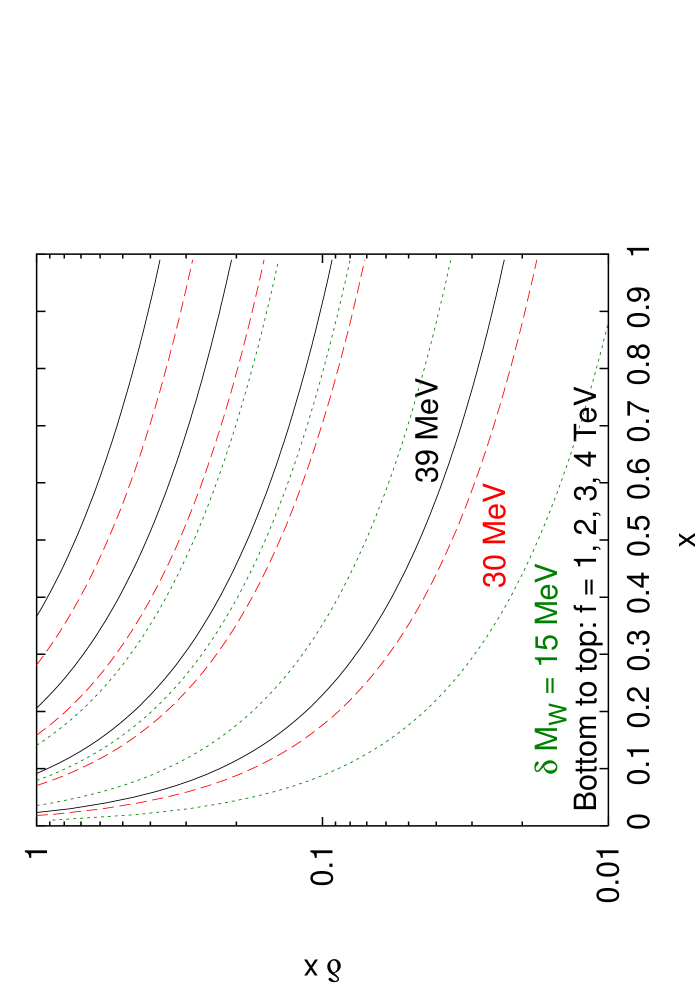
Figure 3: Left: Precision on $x$ required for $\delta R/R_{\rm SM}=1\%$. The solid lines are for $f=1$, 2, 3, 4 TeV (bottom to top). Right: Precision on $x$ obtainable from $M_{W}$ measurement once the other model parameters are known, for the current precision, $\delta M_{W}=39$ MeV (black solid lines), and the goals for Tevatron Run II (2 fb^-1), $\delta M_{W}=30$ MeV (red long-dashed lines), and the LHC (10 fb^-1), $\delta M_{W}=15$ MeV (green short-dashed lines), with $f=1$, 2, 3, 4 TeV (bottom to top for each line type). Note the different scales on the $y$-axis.

A rough measurement of this parameter is needed if $f$ is relatively low.

The ideal place to measure $x$ is in the scalar triplet sector. The mass of the scalar triplet depends on $x$ as given in Eq. (9). The doubly-charged member of the scalar triplet, $\Phi^{++}$, can also be produced in resonant like-sign $WW$ scattering, $W^{+}W^{+}\to\Phi^{++}\to W^{+}W^{+}$ LHpheno with a cross section proportional to $x^{2}v^{4}/f^{2}$. Unfortunately, the cross section is quite small because of the $v^{2}/f^{2}$ suppression, and is not likely to be visible above background ATLASLH .

Alternatively, $x$ can be measured through its effects on electroweak precision observables Kilian . We consider for example the $W$ boson mass. The $W$ boson mass receives a correction in the Littlest Higgs model given at tree level to order $v^{2}/f^{2}$ by

$$M_{W}^{\rm LH} = M_{W}^{\rm SM}\frac{y_{M_{W}}y_{c_{W}}}{y_{M_{Z}}}$$ (17)

$$= M_{W}^{\rm SM}\left\{1+\frac{v^{2}}{2f^{2}}\left[-\frac{s_{W}^{2}}{c_{W}^{2}-s_{W}^{2}}c^{2}s^{2}+\frac{c_{W}^{2}}{c_{W}^{2}-s_{W}^{2}}\left(\frac{5}{4}\left(c^{\prime 2}-s^{\prime 2}\right)^{2}-\frac{1}{4}x^{2}\right)\right]\right\}.$$

If the parameters $f$, $c$, and $c^{\prime}$ (alternatively $f$, $M_{Z_{H}}$, and $M_{A_{H}}$) are known, $x$ can be extracted from the measurement of $M_{W}$ with a precision given by

$$\delta x=\frac{\delta M_{W}}{M_{W}^{\rm SM}}\frac{4f^{2}}{v^{2}x}\frac{c^{2}_{W}-s^{2}_{W}}{c^{2}_{W}}.$$ (18)

This precision is shown in the right panel of Fig. 3 for the current $M_{W}$ measurement, $\delta M_{W}=39$ MeV PDG , and for the expected precisions obtainable with 2 fb^-1 of data in Run II of the Tevatron, $\delta M_{W}=30$ MeV (per experiment) MWBaur ; MWTev , and with 10 fb^-1 of data at the LHC, $\delta M_{W}\simeq 15$ MeV (combining two experiments and multiple channels) MWBaur ; MWLHC . Even the current $M_{W}$ measurement gives enough precision on $x$ to meet the requirement of $\delta R/R_{\rm SM}=1\%$ if the parameters $f$, $c$, and $c^{\prime}$ are known, except for low $x\lesssim 0.05$ for $f=1$ TeV.

We next consider the scale parameter $f$. The sensitivity of $\gamma\gamma\to H\to b\bar{b}$ to $f$ depends on the parameterization and the values of the other parameters. In the first parameterization ($c_{t}$, $x$, $f$, $c$, $c^{\prime}$), the sensitivity to $f$ depends on the parameters $x$, $c$ and $c^{\prime}$, while in the second parameterization ($c_{t}$, $x$, $f$, $M_{Z_{H}}$, $M_{A_{H}}$), the sensitivity to $f$ depends only on the parameter $x$. This is due to the parameter dependence of the terms multiplying $1/f^{2}$ in the expressions for $y_{i}$ given in the Appendix.

In Fig. 4 we show the precision with which $f$ must be measured to give $\delta R/R_{\rm SM}=1\%$ in the second parameterization.

Figure 4: Precision on $f$ required for $\delta R/R_{\rm SM}=1\%$ in the second parameter set ($c_{t}$, $x$, $f$, $M_{Z_{H}}$, $M_{A_{H}}$) for the model with an $A_{H}$ particle (dashed lines) and the model with no $A_{H}$ particle (solid lines). Left: Precision on $f$ as a function of $x$, for $f=1$, 2, 3, 4 TeV (bottom to top for each line type). Right: Precision on $f$ as a function of $f$, for $x=0.37$.

The strongest $f$ dependence (and thus the highest precision desired) occurs for $x\simeq 0.37$, as can be seen in the left panel of Fig. 4. In the right panel of Fig. 4 we show the precision with which $f$ must be measured as a function of $f$, taking $x=0.37$ to conservatively give the strongest $f$ dependence. The electroweak precision data constrain the scale $f$ to be no smaller than about 1 TeV GrahamEW2 . From the right panel of Fig. 4, $f=1$ TeV corresponds to a required precision of $\delta f/f\leq 7\%$. For $f>3.5$ TeV, the precision $\delta f/f$ required to give $\delta R/R_{\rm SM}=1\%$ is greater than one, meaning that knowing that $0<f<7$ TeV is sufficient. However, for such high $f$ values, the correction to the rate for $\gamma\gamma\to H\to b\bar{b}$ due to the Littlest Higgs model is comparable in size to the $1\sigma$ experimental resolution LHloop , and the measurement loses its usefulness as a test of the model.

In the first parameterization, the $f$ dependence is slightly stronger than that shown in Fig. 4. This drives our choice of the input parameter set: by choosing to work in the second parameterization, we reduce the precision with which $f$ must be determined. In addition, we trade two mixing angles, $c$ and $c^{\prime}$, whose values must be extracted from a combination of measurements, for the masses of two heavy gauge bosons, $M_{Z_{H}}$ and $M_{A_{H}}$, which can be measured directly.

How can $f$ be measured at the LHC? The most obvious approach is to extract $f$ from the measurements of the $Z_{H}$ mass and cross section. The $Z_{H}$ mass depends on $f$ and $c$ as given in Eq. (8). The $Z_{H}$ will most likely be discovered in Drell-Yan production with decays to $e^{+}e^{-}$ or $\mu^{+}\mu^{-}$. For fixed $M_{Z_{H}}$, the rate for $pp\to Z_{H}\to\ell^{+}\ell^{-}$ depends strongly on the parameter $c$ through both the production cross section (proportional to $\cot^{2}\theta$) and the decay branching ratio of $Z_{H}$ to dileptons Burdman ; LHpheno . Neglecting the masses of the final-state particles compared to $M_{Z_{H}}$, the $Z_{H}$ partial width into a pair of fermions is given by

$$\Gamma(Z_{H}\to f\bar{f})=\frac{N_{c}g^{2}\cot^{2}\theta}{96\pi}M_{Z_{H}},$$ (19)

where $N_{c}$ = 3 for quarks and 1 for leptons, and the partial width into boson pairs is given by

$$\Gamma(Z_{H}\to ZH)=\Gamma(Z_{H}\to WW)=\frac{g^{2}\cot^{2}2\theta}{192\pi}M_{Z_{H}}.$$ (20)

In our numerical calculations of $Z_{H}$ branching fractions we ignore the masses of all final-state particles except for the top quark.

In Fig. 5 we show the cross section for $Z_{H}$ times its branching ratio into dielectrons as a function of $f$.

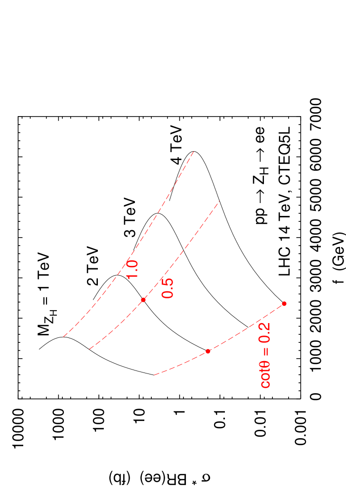
Figure 5: Cross section times branching ratio for $Z_{H}$ into dielectrons at the LHC as a function of $f$. The solid black lines are contours of constant $M_{Z_{H}}$, while the dashed red lines are contours of constant $\cot\theta$.

Electroweak precision data requires $f\gtrsim 1$ TeV and $M_{Z_{H}}\gtrsim 2$ TeV Kilian ; GrahamEW1 ; JoAnneEW ; GrahamEW2 . Perturbativity of the two SU(2) gauge couplings, $g_{1,2}\lesssim\sqrt{4\pi}$, requires $\cot\theta\gtrsim 0.18$. With these constraints, a wide range of cross sections are allowed.

A measurement of the $Z_{H}$ cross section times its branching ratio into dielectrons (from counting events) can be combined with a measurement of $M_{Z_{H}}$ (from the dielectron invariant mass) to extract $f$. To illustrate the prospects for measuring $f$, we study three benchmark points:

• Point 1: $M_{Z_{H}}=2$ TeV, $\cot\theta=0.2$, corresponding to $f=1180$ GeV;

• Point 2: $M_{Z_{H}}=2$ TeV, $\cot\theta=0.5$, corresponding to $f=2454$ GeV;

• Point 3: $M_{Z_{H}}=4$ TeV, $\cot\theta=0.2$, corresponding to $f=2360$ GeV.

The $f$ extraction from the cross section measurement is illustrated for Points 1 and 2 in Fig. 6.

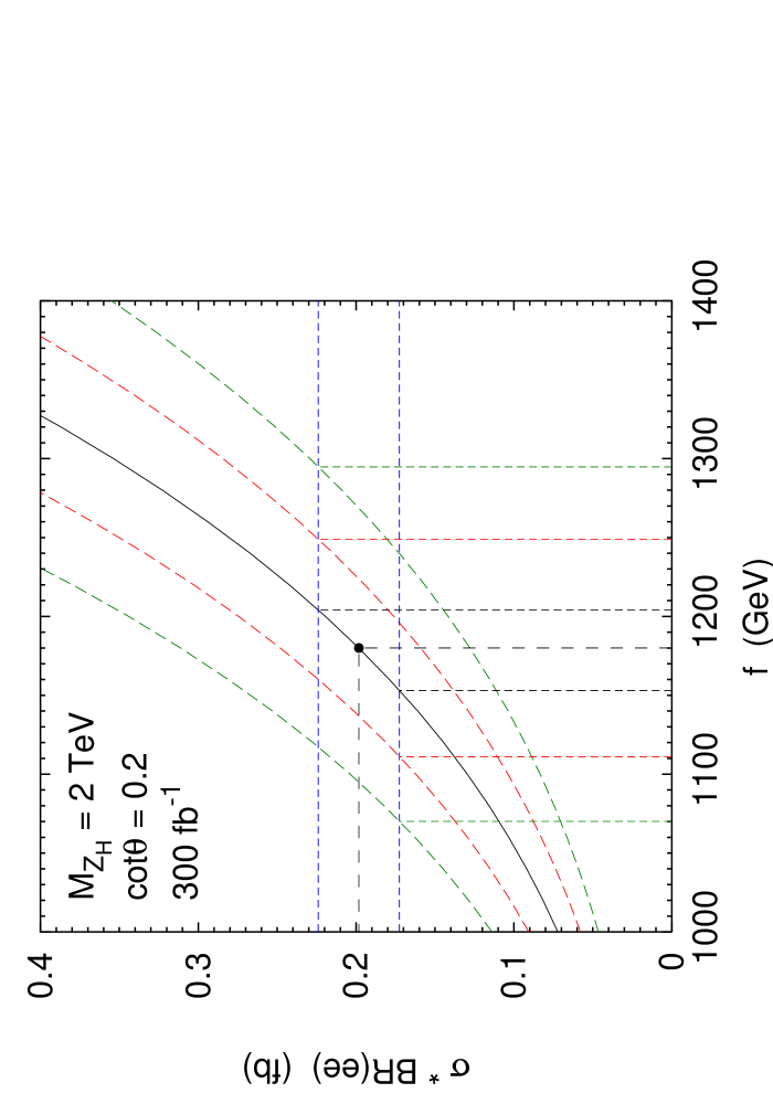
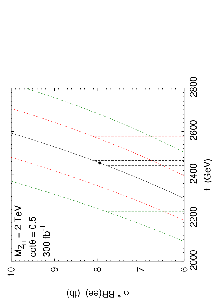
Figure 6: Cross section times branching ratio for $Z_{H}$ into dielectrons at the LHC for Points 1 (left) and 2 (right) discussed in the text (black dots). The solid black line is the contour of $M_{Z_{H}}=2$ TeV. The dashed red and green lines are contours of $M_{Z_{H}}=2$ TeV $\pm 2\%$ and 4%, respectively, and show the effect of the finite $M_{Z_{H}}$ mass resolution on the $f$ determination. The horizontal short-dashed blue lines show the $1\sigma$ statistical uncertainty in the cross section, assuming 100% acceptance and 300 fb^-1 of data.

The resulting uncertainty $\delta f/f$ is summarized in Table 3.

		Statistical uncertainty	$\delta f/f$			Desired $\delta f/f$
	$f$ (GeV)	on $\sigma\times{\rm BR}(ee)$	($\delta M_{Z_{H}}=0$)	($2\%$)	($4\%$)	(no $A_{H}$/with $A_{H}$)
Point 1	1180	13% (59 evts)	2%	6%	10%	10% / 12%
Point 2	2454	2.0% (2380 evts)	0.5%	5%	9%	43% / 49%
Point 3	2360	– (0.8 evts)	–	–	–	40% / 45%

Table 3: Extraction of $f$ from the $Z_{H}$ mass and rate in dielectrons for the three points discussed in the text. The statistical uncertainty on the cross section times branching ratio is calculated from the number of dielectron events assuming 100% acceptance and 300 fb^-1 of data. The effect of the $M_{Z_{H}}$ measurement uncertainty is also shown for $\delta M_{Z_{H}}/M_{Z_{H}}=0$, 2% and 4%. The desired $\delta f/f$ is taken from Fig. 4 for the versions of the model without and with an $A_{H}$ boson.

It is possible to achieve the desired precision on $f$ to give $\delta R/R_{\rm SM}=1\%$ (Fig. 4) over a large part of the parameter space. For Points 1 and 2, the uncertainty in the $M_{Z_{H}}$ measurement dominates the uncertainty in $f$ for $\delta M_{Z_{H}}\gtrsim 2\%$. To match the desired precision for the low $f\sim 1.2$ TeV of Point 1, a fairly high precision measurement of the $Z_{H}$ mass, $\delta M_{Z_{H}}/M_{Z_{H}}\sim 4\%$, is required. Point 3 was chosen as a worst-case scenario with very small cross section yet a moderate value of $f\sim 2.3$ TeV. At this parameter point $Z_{H}$ will not be detected at the LHC in dileptons since the number of events is too small. The bosonic decay modes have larger branching fractions at this point Burdman ; LHpheno , but the $Z_{H}$ is still unlikely to be detected in the bosonic channels for the parameters of Point 3 ATLASLH .

In Fig. 6 and Table 3 the statistical uncertainty on the cross section times branching ratio is taken as $\sqrt{N_{S}}$ for $N_{S}$ signal events. The number of signal events we take to be $\sigma\times{\rm BR}(ee)\times 300$ fb^-1; that is, we assume 100% acceptance for dielectron events in the $Z_{H}$ mass window on top of negligible background. This is of course optimistic; however, very minimal cuts should be needed for the $Z_{H}$ reconstruction in dileptons. The statistics used in Fig. 6 and Table 3 can be doubled by including the dimuon channel, and doubled again by including data from both of the two LHC detectors.

Finally we consider the masses of the heavy gauge bosons $Z_{H}$ and $A_{H}$, shown in Fig. 7.

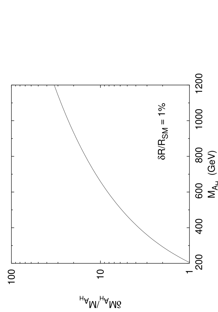
Figure 7: Precision on $M_{Z_{H}}$ (left) and $M_{A_{H}}$ (right) required for $\delta R/R_{\rm SM}=1\%$.

Because the $M_{Z_{H}}$ ($M_{A_{H}}$) dependence of the corrections to the Higgs couplings can be separated from that of the other parameters, the precision needed on $M_{Z_{H}}$ ($M_{A_{H}}$) is independent of the other parameter values.

The electroweak precision data constrain the masses of the heavy SU(2) gauge bosons $Z_{H}$, $W_{H}^{\pm}$ to be no lighter than about 2 TeV GrahamEW1 ; JoAnneEW ; GrahamEW2 . From the left panel of Fig. 7, the precision $\delta M_{Z_{H}}/M_{Z_{H}}$ required to give $\delta R/R_{\rm SM}=1\%$ is greater than one, meaning that only a very rough knowledge of this parameter is required. In particular, even for $M_{Z_{H}}=1$ TeV, $M_{Z_{H}}$ need only be known within a factor of three. This precision will be trivial to achieve. The requirement on the $Z_{H}$ mass measurement for the extraction of $f$ is much more stringent.

If the model contains an $A_{H}$ gauge boson, a measurement of its mass will only be important if it is lighter than about 200 GeV. For a heavier $A_{H}$, the precision $\delta M_{A_{H}}/M_{A_{H}}$ required to give $\delta R/R_{\rm SM}=1\%$ is greater than one (right panel of Fig. 7).

VI Other uncertainties

In addition to the parametric uncertainties in the calculation of the rate for $\gamma\gamma\to H\to b\bar{b}$, we must consider other sources of uncertainty. In this section we discuss potential theoretical and experimental uncertainties in the Littlest Higgs model parameter extraction, issues in the extraction of $\Gamma_{\gamma}\times{\rm BR}(H\to b\bar{b})$ from photon collider measurements, and the sources of uncertainty in the SM Higgs coupling calculation.

VI.1 Littlest Higgs parameter extraction

We have computed the correction to the Higgs partial widths working to leading nontrivial order in the expansion of the Littlest Higgs nonlinear sigma model in powers of $v^{2}/f^{2}$. Higher-order corrections to the Higgs partial widths from the $v^{2}/f^{2}$ expansion are unlikely to be relevant. Higher-order corrections to the parameter translations (e.g., $f,c\leftrightarrow M_{Z_{H}}$) and parameter extractions from LHC data, however, could be important. Their effects on the parameter extraction will be at the few-percent level, which is relevant in particular for the $Z_{H}$ mass in the extraction of $f$ at low $f$ values. These higher-order terms in the expansion are straightforward to include.

QCD corrections to the cross section for $Z_{H}$ production at the LHC must be taken into account in the determination of the $f$ scale. These can be taken over directly from the SM computations for $Z,\gamma$-mediated Drell-Yan. The next-to-leading order (NLO) QCD corrections to Drell-Yan were computed some 25 years ago DYNLO and yield $K$-factors of order 1.4. With the computation of the inclusive NNLO $K$-factor more than ten years ago DYNNLO and the recent computation of the differential NNLO cross section within the past year DYNNLOdiff , the QCD uncertainty in the $Z_{H}$ cross section is well under control. Similarly, the (relatively small) QCD corrections to the $Z_{H}$ branching fraction to dileptons can be taken over from the corresponding calculation for $Z$ decays. In addition, the LHC luminosity uncertainty will contribute to the uncertainty in the $Z_{H}$ cross section. However, a quick examination of Table 3 reveals that even a $\sim 10\%$ (statistical) uncertainty on the $Z_{H}$ production cross section times leptonic branching ratio does not contribute significantly to the uncertainty in $f$, so that these systematic uncertainties are not a problem.

More important for the determination of $f$ are the corrections to, and measurement uncertainties of, the $Z_{H}$ boson mass. For $f\sim 1$ TeV, a measurement of $M_{Z_{H}}$ at the $\sim 4\%$ level is desirable. At this level of precision, electroweak radiative corrections to the $Z_{H}$ mass could be important. To be more precise, the parameter translations between LHC measurements, Littlest Higgs model parameters, and the $\gamma\gamma\to H\to b\bar{b}$ rate may need to be treated at next-to-leading order in the electroweak couplings. This could also be important for the parameter $x$ at low $f\sim 1$ TeV, which we have proposed to extract from the $W$ boson mass measurement. Radiative corrections to the $W$ mass within the Littlest Higgs model could be important for this extraction; in particular, because the model contains a scalar triplet that gets a nonzero vev, violating custodial symmetry at the tree level, the renormalization of the electroweak sector at the one-loop level requires one additional input (to fix the triplet vev counterterm) beyond the usual three SM inputs phivev ; Sally . This extra input parameter can have important effects on the parameter dependence of the one-loop corrections to the SM observables Sally ; phivev2 . The first one-loop calculation in the Littlest Higgs model involving renormalization of the electroweak sector was done in Ref. Sally .

There are also experimental issues in the measurement of the $Z_{H}$ mass to high precision, which have been discussed, e.g., in Ref. LesHouches . The measurement of the mass of a new heavy (TeV-scale) gauge boson at the LHC relies on accurate measurements of the energy/momentum of very high-energy electrons or muons. For the $Z_{H}$ masses considered ($\geq 2$ TeV), these leptons will have energies of 1 TeV or higher. For electrons, the energy measurement will come primarily from the electromagnetic calorimeter. Uncertainties come from both the energy resolution and the energy scale calibration. A calibration of the lepton energy scale at TeV-scale energies could be made, e.g., using very high-$p_{T}$ $Z$ bosons decaying to dielectrons. For muons, the momentum is measured from track curvature. While the calibration is under control here, the energy resolution per event is worse because the tracks are very stiff, so higher statistics may be needed. Since many models of TeV-scale new physics contain high-mass resonances that decay to dileptons, we feel that a more detailed study of the systematic uncertainties affecting the $Z^{\prime}$ mass measurement would be worthwhile.

VI.2 Photon collider issues

Photon collider studies ggAsner ; LeptonPhoton ; AGG ; Jikia ; Krawczyk1 ; Krawczyk2 ; Rosca claim a 2% measurement of the $\gamma\gamma\to H\to b\bar{b}$ rate, which we interpret as a measurement of $\Gamma_{\gamma}\times{\rm BR}(H\to b\bar{b})$. We mention here some sources of uncertainty that must be under control before such a high precision measurement is claimed.

First, the $\gamma\gamma$ luminosity and polarization spectra must be measured to normalize the Higgs production rate. The photon and electron luminosity and polarization spectra are currently simulated using the programs CAIN CAIN and GUINEA-PIG GUINEA-PIG . The luminosity spectrum can be measured using the reactions $\gamma\gamma\to e^{+}e^{-}$ gglumipol and perhaps $\gamma\gamma\to e^{+}e^{-}\gamma$. The photon polarization spectrum could be measured using $e\gamma\to e\gamma$ and $e\gamma\to W\nu$ TESLATDR ; ggAsner . Further study is needed.

Second, a photon collider collides more than just photons. The photon has a parton distribution function containing quarks, gluons, etc., and collisions of such “resolved” photons can yield Higgs production via, e.g., gluon fusion or $b\bar{b}$ fusion. This resolved-photon part of the Higgs production cross section is not proportional to $\Gamma_{\gamma}$. The resolved photon contribution to SM Higgs production has been studied in Ref. Doncheski for a photon collider with $\sqrt{s}_{ee}=500$ GeV and found to be at the percent level or smaller. Similarly, the remnant electron beams can contribute to Higgs production via $ZZ$ fusion, $e^{-}e^{-}\to e^{-}e^{-}Z^{*}Z^{*}\to e^{-}e^{-}H$. These contributions to Higgs production are likely to be small, but a quantitative estimate would be useful.

Finally, the background to $\gamma\gamma\to H\to b\bar{b}$ consists mostly of $b\bar{b}(g)$ production, with some $c\bar{c}(g)$ contribution from charm quarks mistagged as bottom. The signal is peaked at the Higgs mass on top of a background steeply falling with increasing two-jet invariant mass (due to the photon beam energy spectrum). The background can be simulated based on the beam spectra CAIN ; GUINEA-PIG and the QCD-corrected cross sections for heavy quark pair production in $\gamma\gamma$ collisions ggtobbg . The background normalization must be under control to subtract from the signal.

VI.3 Standard Model Higgs coupling calculation

In order to predict the rate for $\gamma\gamma\to H\to b\bar{b}$ at the 1% level in the Littlest Higgs model, the SM rate must be known at the same level of precision. We outline here the known radiative corrections and sources of uncertainty in the SM prediction.

The SM $H\to\gamma\gamma$ decay partial width receives QCD corrections, which of course only affect the top-quark diagrams. Because the external particles in the $\gamma\gamma H$ vertex are color neutral, the virtual QCD corrections are finite by themselves. Since no real radiation diagrams contribute, the QCD corrections to $H\to\gamma\gamma$ are equivalent to those to the inverse process $\gamma\gamma\to H$. This is in contrast to, e.g., the QCD corrections to the $ggH$ vertex.

The QCD corrections to $\Gamma_{\gamma}$ in the SM are known analytically at the two-loop [$\mathcal{O}(\alpha_{s})$] order ggH2loopQCD and as a power expansion up to third order in $M_{H}/m_{t}$ at three-loop [$\mathcal{O}(\alpha_{s}^{2})$] order ggH3loopQCD . They are small for Higgs masses $M_{H}<2m_{t}$; the $\mathcal{O}(\alpha_{s})$ corrections are only of order 2% for $M_{H}<2M_{W}$, and the $\mathcal{O}(\alpha_{s}^{2})$ corrections are negligible, demonstrating that the QCD corrections are well under control.

The SM $H\to\gamma\gamma$ decay partial width also receives electroweak radiative corrections. The the electroweak corrections are much more difficult to compute than the QCD corrections and a full two-loop calculation does not yet exist. The electroweak correction due to two-loop diagrams containing light fermion loops and $W$ or $Z$ bosons (with the Higgs boson coupled to the $W$ or $Z$ boson, because the light fermion Yukawa couplings are neglected) was computed recently in Ref. ggHEWlightf and contributes between $-1\%$ and $-2\%$ for $M_{H}\lesssim 140$ GeV. The leading $\mathcal{O}(G_{F}m_{t}^{2})$ electroweak correction due to top-mass-enhanced two-loop diagrams containing third-generation quarks was also computed recently in Ref. ggHEWGFmt2 as an expansion to fourth order in the ratio $M_{H}^{2}/(2M_{W})^{2}$. The expansion appears to be under good control for $M_{H}\lesssim 140$ GeV, where this correction contributes about $-2.5\%$ almost independent of $M_{H}$. We conclude that the electroweak radiative corrections to $\gamma\gamma\to H$ appear to be under control at the 1–2% level.

We now consider the uncertainty in the SM prediction for the $H\to b\bar{b}$ branching ratio. The radiative corrections to Higgs decays to fermion and boson pairs have been reviewed in Ref. Spirareview ; we give here a brief sketch of the known corrections and refer to Ref. Spirareview for references to the original calculations. The full QCD corrections to the Higgs decay to $q\bar{q}$ are known up to three loops neglecting the quark mass in the kinematics and up to two loops for massive final-state quarks. The electroweak corrections to the Higgs decay to quark or lepton pairs are known at one-loop; in addition, the QCD corrections to the leading top-mass-enhanced electroweak correction term are known up to three loops, to order $G_{F}m_{t}^{2}\alpha_{s}^{2}$. All of these corrections to the Higgs partial widths to fermions are included in a consistent way in the program HDECAY HDECAY .

For the Higgs masses below the $WW$ threshold that we consider here, decays into off-shell gauge bosons ($WW$, $ZZ$) are important and affect the total Higgs width, thus feeding in to ${\rm BR}(H\to b\bar{b})$. HDECAY takes into account decays with both $W$ ($Z$) bosons off-shell. One-loop electroweak corrections to Higgs decays to $WW$ and $ZZ$ are known, together with the QCD corrections to the leading $\mathcal{O}(G_{F}m_{t}^{2})$ result up to three loops. These corrections to $\Gamma_{W,Z}$ amount to less than about 5% in the intermediate Higgs mass range Spirareview (translating to less than roughly 2% in ${\rm BR}(H\to b\bar{b})$ for $M_{H}\simeq 120$ GeV) and have been neglected in HDECAY, although their inclusion would seem straightforward.

The $H\to b\bar{b}$ branching ratio in the SM also has a parametric uncertainty due to the nonzero present experimental uncertainties in the SM input parameters. The largest sources of parametric uncertainty are the bottom quark mass and (to a lesser extent) the strong coupling $\alpha_{s}$ (which contributes via the QCD corrections to the $Hb\bar{b}$ coupling). This parametric uncertainty in ${\rm BR}(H\to b\bar{b})$ was evaluated in Ref. MSSMHiggs to be about 1.4% for $M_{H}=120$ GeV, using the standard $\alpha_{s}=0.1185\pm 0.0020$ alphas and a somewhat optimistic $m_{b}(m_{b})=4.17\pm 0.05$ GeV ($\overline{\rm MS}$) mbmb . The parametric uncertainty in the branching ratio is suppressed due to the fact that $\Gamma_{b}$ makes up about 2/3 of the Higgs total width at $M_{H}=120$ GeV, leading to a partial cancellation of the uncertainty in the branching ratio; we thus expect the parametric uncertainty to be somewhat larger at higher Higgs masses, where $\Gamma_{b}$ no longer dominates the total width.

The best measurements of $\alpha_{s}$ come from LEP-I and II; the Tevatron and LHC are unlikely to improve on this. The bottom quark mass is extracted from heavy quarkonium spectroscopy and $B$ meson decays with a precision limited by theoretical uncertainty. There are prospects to improve the bottom quark mass extraction through better perturbative and lattice calculations bottommass and more precise measurements of the upsilon meson properties from CLEO CLEO .

VII Conclusions

We have calculated the $\mathcal{O}(v^{2}/f^{2})$ corrections to the partial widths of the light Higgs boson in the Littlest Higgs model. These results allow numerical calculations of the corrections to the Higgs boson total width and decay branching ratios, as well as the corrections to the Higgs boson production cross section in two-photon fusion and in gluon fusion. We studied the correction to the rate of $\gamma\gamma\to H\to b\bar{b}$, which is expected to be measured at a future photon collider with 2% precision for a light Higgs boson with mass in the range $115-140$ GeV.

For $f\sim 1$ TeV, the correction to the $\gamma\gamma\to H\to b\bar{b}$ rate is roughly $-6\%$. In order to make a theoretical prediction for the corrected rate $R=R_{\rm SM}+R_{\rm LH}$ with 1% precision (i.e., a theoretical uncertainty comfortably smaller than the experimental uncertainty of 2%), the correction $R_{\rm LH}$ need only be computed at the $15\%$ level for $f\sim 1$ TeV. We studied the precision with which the Littlest Higgs model parameters must be measured in order to match the photon collider precision, and conclude that measurements of the model parameters with high enough precision should be possible at the LHC over much of the relevant model parameter space.

The measurement of $\gamma\gamma\to H\to b\bar{b}$ provides a nontrivial test of the Littlest Higgs model. More interestingly, it also provides a probe of the UV completion of the nonlinear sigma model at the 10 TeV scale. The loop-induced Higgs coupling to photon pairs, for example, can receive corrections from the new heavy particles of the UV completion running in the loop. Equivalently, the dimension-6 operator $h^{\dagger}hF^{\mu\nu}F_{\mu\nu}/\Lambda^{2}$ that gives rise to the $\gamma\gamma H$ coupling receives a contribution from the 10 TeV scale. If the UV completion is weakly coupled, these corrections will be suppressed by the square of the ratio of the electroweak scale to the 10 TeV scale, and thus be too small to detect with the expected 2% experimental resolution. If the UV completion is strongly coupled, however, the strong-coupling enhancement counteracts the suppression from the high mass scale, leading to corrections parametrically of the same order as those from the TeV scale physics that should be observable at the photon collider.

Appendix A

The partial width of the Higgs boson into two photons is given in the Littlest Higgs model by LHloop ; HHG

$$\Gamma_{\gamma}=\frac{\sqrt{2}G_{F}\alpha^{2}M_{H}^{3}y^{2}_{G_{F}}}{256\pi^{3}}\left|\sum_{i}y_{i}N_{ci}Q_{i}^{2}F_{i}\right|^{2},$$ (21)

where $N_{ci}$ and $Q_{i}$ are the color factor ($=1$ or 3) and electric charge, respectively, for each particle $i$ running in the loop. The standard dimensionless loop factors $F_{i}$ for particles of spin 1, 1/2, and 0 are given in Ref. HHG . The factors $y_{i}$ in the sum incorporate the couplings and mass suppression factors of the particles running in the loop. For the top quark and $W$ boson, whose couplings to the Higgs boson are proportional to their masses, the $y_{i}$ factors are equal to one up to a correction of order $v^{2}/f^{2}$ LHloop . For the TeV-scale particles in the loop, on the other hand, the $y_{i}$ factors are of order $v^{2}/f^{2}$. This reflects the fact that the masses of the heavy particles are not generated by their couplings to the Higgs boson; rather, they are generated by the $f$ condensate. This behavior naturally respects the decoupling limit for physics at the scale $f\gg v$.

Normalizing the Higgs partial width into photons to its SM value, we have

$$\Gamma_{\gamma}/\Gamma_{\gamma}^{\rm SM}=y^{2}_{G_{F}}\frac{\left|\sum_{i,{\rm LH}}y_{i}N_{ci}Q_{i}^{2}F_{i}\right|^{2}}{\left|\sum_{i,{\rm SM}}N_{ci}Q_{i}^{2}F_{i}\right|^{2}},$$ (22)

where $i$ runs over the fermions in the loop: $t$, $T$, $W$, $W_{H}$, and $\Phi^{+}$ in the Littlest Higgs (LH) case; and $t$ and $W$ in the SM case.

The partial width of the Higgs boson into two gluons, normalized to its SM value, is given in the Littlest Higgs model by HHG ; LHloop

$$\Gamma_{g}/\Gamma_{g}^{\rm SM}=y^{2}_{G_{F}}\frac{\left|\sum_{i,{\rm LH}}y_{i}F_{1/2}(\tau_{i})\right|^{2}}{\left|\sum_{i,{\rm SM}}F_{1/2}(\tau_{i})\right|^{2}},$$ (23)

where $i$ runs over the fermions in the loop: $t$ and $T$ in the Littlest Higgs case, and $t$ in the SM case. The dimensionless loop factor $F_{1/2}$ is again given in Ref. HHG .

We now list the formulas for the correction factors $y_{i}$ in terms of two sets of input parameters:

1. $c_{t}$, $x$, $f$, $c$, $c^{\prime}$, and

2. $c_{t}$, $x$, $f$, $M_{Z_{H}}$, $M_{A_{H}}$.

For the model in which two U(1) groups are gauged, leading to an $A_{H}$ particle in the spectrum, we have:

$$y^{2}_{G_{F}} = 1+\frac{v^{2}}{f^{2}}\left[-\frac{5}{12}+\frac{1}{4}x^{2}\right]$$ (24)

$$y_{t} = 1+\frac{v^{2}}{f^{2}}\left[-\frac{2}{3}+\frac{1}{2}x-\frac{1}{4}x^{2}+c_{t}^{2}s_{t}^{2}\right]$$ (25)

$$y_{W} = 1+\frac{v^{2}}{f^{2}}\left[-\frac{1}{6}-\frac{1}{4}(c^{2}-s^{2})^{2}\right]$$ (26)

$$= 1+\frac{v^{2}}{f^{2}}\left[-\frac{5}{12}\right]+\frac{M_{W}^{2}}{M_{Z_{H}}^{2}}$$

$$y_{T} = -c_{t}^{2}s_{t}^{2}\frac{v^{2}}{f^{2}}$$ (27)

$$y_{W_{H}} = -s^{2}c^{2}\frac{v^{2}}{f^{2}}$$ (28)

$$= -\frac{M_{W}^{2}}{M_{Z_{H}}^{2}}$$

$$y_{\Phi^{+}} = \frac{v^{2}}{f^{2}}\left[-\frac{1}{3}+\frac{1}{4}x^{2}\right]$$ (29)

$$y_{\Phi^{++}} = 0$$ (30)

$$y_{f} = 1+\frac{v^{2}}{f^{2}}\left[-\frac{2}{3}+\frac{1}{2}x-\frac{1}{4}x^{2}\right]$$ (31)

$$y_{Z} = 1+\frac{v^{2}}{f^{2}}\left[-\frac{1}{6}-\frac{1}{4}(c^{2}-s^{2})^{2}-\frac{5}{4}(c^{\prime 2}-s^{\prime 2})^{2}+\frac{1}{4}x^{2}\right]$$ (32)

$$= 1+\frac{v^{2}}{f^{2}}\left[-\frac{5}{3}+\frac{1}{4}x^{2}\right]+\frac{M_{W}^{2}}{M_{Z_{H}}^{2}}+\frac{s_{W}^{2}}{c_{W}^{2}}\frac{M_{W}^{2}}{M_{A_{H}}^{2}}$$

$$y^{2}_{M_{Z}} = 1+\frac{v^{2}}{f^{2}}\left[-\frac{1}{6}-\frac{1}{4}(c^{2}-s^{2})^{2}-\frac{5}{4}(c^{\prime 2}-s^{\prime 2})^{2}+\frac{1}{2}x^{2}\right]$$ (33)

$$= 1+\frac{v^{2}}{f^{2}}\left[-\frac{5}{3}+\frac{1}{2}x^{2}\right]+\frac{M_{W}^{2}}{M_{Z_{H}}^{2}}+\frac{s_{W}^{2}}{c_{W}^{2}}\frac{M_{W}^{2}}{M_{A_{H}}^{2}}$$

$$y^{2}_{M_{W}} = 1+\frac{v^{2}}{f^{2}}\left[-\frac{1}{6}-\frac{1}{4}(c^{2}-s^{2})^{2}+\frac{1}{4}x^{2}\right]$$ (34)

$$= 1+\frac{v^{2}}{f^{2}}\left[-\frac{5}{12}+\frac{1}{4}x^{2}\right]+\frac{M_{W}^{2}}{M_{Z_{H}}^{2}}$$

$$y^{2}_{c_{W}} = 1+\frac{v^{2}}{f^{2}}\frac{s^{2}_{W}}{c^{2}_{W}-s^{2}_{W}}\left[-\frac{1}{4}+\frac{1}{4}(c^{2}-s^{2})^{2}+\frac{5}{4}(c^{\prime 2}-s^{\prime 2})^{2}-\frac{1}{4}x^{2}\right]$$ (35)

$$= 1+\frac{v^{2}}{f^{2}}\frac{s^{2}_{W}}{c^{2}_{W}-s^{2}_{W}}\left[\frac{5}{4}-\frac{1}{4}x^{2}\right]+\frac{s_{W}^{2}}{c_{W}^{2}-s_{W}^{2}}\left[-\frac{M_{W}^{2}}{M_{Z_{H}}^{2}}-\frac{s_{W}^{2}}{c_{W}^{2}}\frac{M_{W}^{2}}{M_{A_{H}}^{2}}\right].$$

In Eq. (30), the $\Phi^{++}\Phi^{--}H$ coupling is zero at leading order in $v^{2}/f^{2}$ LHloop , so the corresponding $y_{\Phi^{++}}$ is suppressed by an extra factor of $v^{2}/f^{2}$ and we thus ignore it. The $f\bar{f}H$ coupling in Eq. (31) was given previously in Eq. (B.10) of Ref. Deandrea ; after correcting a typo Deandreaprivate we reproduce their result.

For the model in which only one U(1) group (hypercharge) is gauged, so that there is no $A_{H}$ particle in the spectrum, the $y_{i}$ factors in terms of the parameters $c_{t}$, $x$, $f$, and $c$ are obtained from Eqs. (24–35) by setting $c^{\prime}=s^{\prime}=1/\sqrt{2}$. The $y_{i}$ factors in terms of the parameters $c_{t}$, $x$, $f$, $M_{Z_{H}}$ are given as above except for

$$y_{Z} = 1+\frac{v^{2}}{f^{2}}\left[-\frac{5}{12}+\frac{1}{4}x^{2}\right]+\frac{M_{W}^{2}}{M_{Z_{H}}^{2}}$$ (36)

$$y^{2}_{M_{Z}} = 1+\frac{v^{2}}{f^{2}}\left[-\frac{5}{12}+\frac{1}{2}x^{2}\right]+\frac{M_{W}^{2}}{M_{Z_{H}}^{2}}$$ (37)

$$y^{2}_{c_{W}} = 1+\frac{v^{2}}{f^{2}}\frac{s_{W}^{2}}{c_{W}^{2}-s_{W}^{2}}\left[-\frac{1}{4}x^{2}\right]-\frac{s_{W}^{2}}{c_{W}^{2}-s_{W}^{2}}\frac{M_{W}^{2}}{M_{Z_{H}}^{2}}.$$ (38)

References

- (1) M. W. Grunewald, arXiv:hep-ex/0304023.
- (2) N. Arkani-Hamed, A. G. Cohen, E. Katz and A. E. Nelson, JHEP 0207, 034 (2002) [arXiv:hep-ph/0206021].
- (3) N. Arkani-Hamed, A. G. Cohen and H. Georgi, Phys. Lett. B 513, 232 (2001) [arXiv:hep-ph/0105239]; N. Arkani-Hamed, A. G. Cohen, E. Katz, A. E. Nelson, T. Gregoire and J. G. Wacker, JHEP 0208, 021 (2002) [arXiv:hep-ph/0206020]; I. Low, W. Skiba and D. Smith, Phys. Rev. D 66, 072001 (2002) [arXiv:hep-ph/0207243]; D. E. Kaplan and M. Schmaltz, JHEP 0310, 039 (2003) [arXiv:hep-ph/0302049]; S. Chang and J. G. Wacker, Phys. Rev. D 69, 035002 (2004) [arXiv:hep-ph/0303001]; W. Skiba and J. Terning, Phys. Rev. D 68, 075001 (2003) [arXiv:hep-ph/0305302]; S. Chang, JHEP 0312, 057 (2003) [arXiv:hep-ph/0306034].
- (4) S. Chang and H. J. He, Phys. Lett. B 586, 95 (2004) [arXiv:hep-ph/0311177].
- (5) A. E. Nelson, arXiv:hep-ph/0304036; E. Katz, J. y. Lee, A. E. Nelson and D. G. E. Walker, arXiv:hep-ph/0312287.
- (6) D. E. Kaplan, M. Schmaltz and W. Skiba, arXiv:hep-ph/0405257.
- (7) T. Han, H. E. Logan, B. McElrath and L. T. Wang, Phys. Rev. D 67, 095004 (2003) [arXiv:hep-ph/0301040].
- (8) T. Han, H. E. Logan, B. McElrath and L. T. Wang, Phys. Lett. B 563, 191 (2003) [arXiv:hep-ph/0302188].
- (9) W. Kilian and J. Reuter, arXiv:hep-ph/0311095.
- (10) R. Casalbuoni, A. Deandrea and M. Oertel, JHEP 0402, 032 (2004) [arXiv:hep-ph/0311038].
- (11) ATLAS Technical Design Report, CERN-LHCC-99-15 (1999); CMS Technical Proposal, CERN-LHCC-94-38 (1994).
-
(12)
D. Zeppenfeld, R. Kinnunen, A. Nikitenko and E. Richter-Was,
Phys. Rev. D 62, 013009 (2000)
[arXiv:hep-ph/0002036];
A. Djouadi et al.,
arXiv:hep-ph/0002258;
A. Belyaev and L. Reina,
JHEP 0208, 041 (2002)
[arXiv:hep-ph/0205270];
M. Dührssen, ATL-PHYS-2003-030, available from
http://cdsweb.cern.ch/; M. Dührssen, S. Heinemeyer, H. Logan, D. Rainwater, G. Weiglein and D. Zeppenfeld, arXiv:hep-ph/0406323. - (13) T. Abe et al. [American Linear Collider Working Group], in Proc. of the APS/DPF/DPB Summer Study on the Future of Particle Physics (Snowmass 2001) ed. N. Graf, arXiv:hep-ex/0106056; K. Abe et al. [ACFA Linear Collider Working Group], arXiv:hep-ph/0109166.
- (14) J. A. Aguilar-Saavedra et al. [ECFA/DESY LC Physics Working Group], arXiv:hep-ph/0106315.
- (15) D. Asner et al., Eur. Phys. J. C 28, 27 (2003) [arXiv:hep-ex/0111056].
- (16) D. Asner et al., arXiv:hep-ph/0308103.
- (17) T. Ohgaki, T. Takahashi and I. Watanabe, Phys. Rev. D 56, 1723 (1997) [arXiv:hep-ph/9703301].
- (18) D. M. Asner, J. B. Gronberg and J. F. Gunion, Phys. Rev. D 67, 035009 (2003) [arXiv:hep-ph/0110320].
- (19) G. Jikia and S. Soldner-Rembold, Nucl. Phys. Proc. Suppl. 82, 373 (2000) [arXiv:hep-ph/9910366]; Nucl. Instrum. Meth. A 472, 133 (2001) [arXiv:hep-ex/0101056].
- (20) P. Niezurawski, A. F. Zarnecki and M. Krawczyk, Acta Phys. Polon. B 34, 177 (2003) [arXiv:hep-ph/0208234].
- (21) P. Niezurawski, A. F. Zarnecki and M. Krawczyk, arXiv:hep-ph/0307183.
- (22) A. Rosca and K. Monig, arXiv:hep-ph/0310036.
- (23) H. Braun, CERN-PS-2000-030-AE Prepared for 7th European Particle Accelerator Conference (EPAC 2000), Vienna, Austria, 26-30 Jun 2000.
- (24) R. W. Assmann et al., CERN-2000-008, SLAC-REPRINT-2000-096.
- (25) P. Niezurawski, A. F. Zarnecki and M. Krawczyk, JHEP 0211, 034 (2002) [arXiv:hep-ph/0207294]; arXiv:hep-ph/0307175.
- (26) E. Asakawa and K. Hagiwara, Eur. Phys. J. C 31, 351 (2003) [arXiv:hep-ph/0305323]; E. Asakawa, S. Y. Choi, K. Hagiwara and J. S. Lee, Phys. Rev. D 62, 115005 (2000) [arXiv:hep-ph/0005313]; E. Asakawa, J. i. Kamoshita, A. Sugamoto and I. Watanabe, Eur. Phys. J. C 14, 335 (2000) [arXiv:hep-ph/9912373].
- (27) A. Djouadi, J. Kalinowski and M. Spira, Comput. Phys. Commun. 108, 56 (1998) [arXiv:hep-ph/9704448].
- (28) A. Manohar and H. Georgi, Nucl. Phys. B 234, 189 (1984); H. Georgi, Phys. Lett. B 298, 187 (1993) [arXiv:hep-ph/9207278].
- (29) C. Csaki, J. Hubisz, G. D. Kribs, P. Meade and J. Terning, Phys. Rev. D 68, 035009 (2003) [arXiv:hep-ph/0303236].
- (30) C. Csaki, J. Hubisz, G. D. Kribs, P. Meade and J. Terning, Phys. Rev. D 67, 115002 (2003) [arXiv:hep-ph/0211124].
- (31) J. L. Hewett, F. J. Petriello and T. G. Rizzo, JHEP 0310, 062 (2003) [arXiv:hep-ph/0211218].
- (32) S. C. Park and J. h. Song, arXiv:hep-ph/0306112.
- (33) M. Perelstein, M. E. Peskin and A. Pierce, Phys. Rev. D 69, 075002 (2004) [arXiv:hep-ph/0310039].
- (34) C. Dib, R. Rosenfeld and A. Zerwekh, arXiv:hep-ph/0302068; C. x. Yue, S. z. Wang and D. q. Yu, Phys. Rev. D 68, 115004 (2003) [arXiv:hep-ph/0309113]; J. J. Liu, W. G. Ma, G. Li, R. Y. Zhang and H. S. Hou, arXiv:hep-ph/0404171.
- (35) R. V. Harlander and W. B. Kilgore, Phys. Rev. Lett. 88, 201801 (2002) [arXiv:hep-ph/0201206]; C. Anastasiou and K. Melnikov, Nucl. Phys. B 646, 220 (2002) [arXiv:hep-ph/0207004].
- (36) M. Carena, H. E. Haber, H. E. Logan and S. Mrenna, Phys. Rev. D 65, 055005 (2002) [Erratum-ibid. D 65, 099902 (2002)] [arXiv:hep-ph/0106116].
- (37) G. Azuelos et al., arXiv:hep-ph/0402037.
- (38) K. Hagiwara et al. [Particle Data Group Collaboration], Phys. Rev. D 66, 010001 (2002).
- (39) U. Baur, arXiv:hep-ph/0304266.
- (40) R. Brock et al., arXiv:hep-ex/0011009.
- (41) S. Haywood et al., arXiv:hep-ph/0003275.
- (42) G. Burdman, M. Perelstein and A. Pierce, Phys. Rev. Lett. 90, 241802 (2003) [Erratum-ibid. 92, 049903 (2004)] [arXiv:hep-ph/0212228].
- (43) G. Altarelli, R. K. Ellis and G. Martinelli, Nucl. Phys. B 143, 521 (1978) [Erratum-ibid. B 146, 544 (1978)]; J. Kubar-Andre and F. E. Paige, Phys. Rev. D 19, 221 (1979).
- (44) R. Hamberg, W. L. van Neerven and T. Matsuura, Nucl. Phys. B 359, 343 (1991) [Erratum-ibid. B 644, 403 (2002)]; R. V. Harlander and W. B. Kilgore, Phys. Rev. Lett. 88, 201801 (2002) [arXiv:hep-ph/0201206].
- (45) C. Anastasiou, L. J. Dixon, K. Melnikov and F. Petriello, Phys. Rev. Lett. 91, 182002 (2003) [arXiv:hep-ph/0306192]; C. Anastasiou, L. Dixon, K. Melnikov and F. Petriello, Phys. Rev. D 69, 094008 (2004) [arXiv:hep-ph/0312266].
- (46) G. Passarino, Nucl. Phys. B 361, 351 (1991); B. W. Lynn and E. Nardi, Nucl. Phys. B 381, 467 (1992).
- (47) M. C. Chen and S. Dawson, arXiv:hep-ph/0311032.
- (48) T. Blank and W. Hollik, Nucl. Phys. B 514, 113 (1998) [arXiv:hep-ph/9703392]; M. Czakon, M. Zralek and J. Gluza, Nucl. Phys. B 573, 57 (2000) [arXiv:hep-ph/9906356]; M. Czakon, J. Gluza, F. Jegerlehner and M. Zralek, Eur. Phys. J. C 13, 275 (2000) [arXiv:hep-ph/9909242].
- (49) G. Azuelos et al., arXiv:hep-ph/0204031.
- (50) P. Chen, G. Horton-Smith, T. Ohgaki, A. W. Weidemann and K. Yokoya, Nucl. Instrum. Meth. A 355, 107 (1995).
- (51) D. Schulte, DESY-TESLA-97-08.
- (52) Y. Yasui, I. Watanabe, J. Kodaira and I. Endo, Nucl. Instrum. Meth. A 335, 385 (1993) [arXiv:hep-ph/9212312].
-
(53)
R. Brinkmann, et al.,
DESY-97-048, available from
http://www-library.desy.de/preparch/desy/1997/desy97-048.html. - (54) M. A. Doncheski and S. Godfrey, Phys. Rev. D 67, 073021 (2003) [arXiv:hep-ph/0105070].
- (55) M. Baillargeon, G. Belanger and F. Boudjema, Phys. Rev. D 51, 4712 (1995) [arXiv:hep-ph/9409263].
- (56) D. L. Borden, V. A. Khoze, W. J. Stirling and J. Ohnemus, Phys. Rev. D 50, 4499 (1994) [arXiv:hep-ph/9405401]; G. Jikia and A. Tkabladze, Nucl. Instrum. Meth. A 355, 81 (1995) [arXiv:hep-ph/9406428]; Phys. Rev. D 54, 2030 (1996) [arXiv:hep-ph/9601384]; M. Melles and W. J. Stirling, Phys. Rev. D 59, 094009 (1999) [arXiv:hep-ph/9807332]; Eur. Phys. J. C 9, 101 (1999) [arXiv:hep-ph/9810432]; M. Melles, W. J. Stirling and V. A. Khoze, Phys. Rev. D 61, 054015 (2000) [arXiv:hep-ph/9907238].
- (57) H. q. Zheng and D. d. Wu, Phys. Rev. D 42, 3760 (1990); A. Djouadi, M. Spira, J. J. van der Bij and P. M. Zerwas, Phys. Lett. B 257, 187 (1991); S. Dawson and R. P. Kauffman, Phys. Rev. D 47, 1264 (1993); A. Djouadi, M. Spira and P. M. Zerwas, Phys. Lett. B 311, 255 (1993) [arXiv:hep-ph/9305335]; K. Melnikov and O. I. Yakovlev, Phys. Lett. B 312, 179 (1993) [arXiv:hep-ph/9302281]; M. Inoue, R. Najima, T. Oka and J. Saito, Mod. Phys. Lett. A 9, 1189 (1994); J. Fleischer, O. V. Tarasov and V. O. Tarasov, Phys. Lett. B 584, 294 (2004) [arXiv:hep-ph/0401090].
- (58) M. Steinhauser, arXiv:hep-ph/9612395.
- (59) U. Aglietti, R. Bonciani, G. Degrassi and A. Vicini, arXiv:hep-ph/0404071.
- (60) F. Fugel, B. A. Kniehl and M. Steinhauser, arXiv:hep-ph/0405232.
- (61) Y. Liao and X. y. Li, Phys. Lett. B 396, 225 (1997) [arXiv:hep-ph/9605310]; A. Djouadi, P. Gambino and B. A. Kniehl, Nucl. Phys. B 523, 17 (1998) [arXiv:hep-ph/9712330].
- (62) J. G. Korner, K. Melnikov and O. I. Yakovlev, Phys. Rev. D 53, 3737 (1996) [arXiv:hep-ph/9508334].
- (63) M. Spira, Fortsch. Phys. 46, 203 (1998) [arXiv:hep-ph/9705337].
- (64) D. E. Groom et al. [Particle Data Group Collaboration], Eur. Phys. J. C 15, 1 (2000).
- (65) A. H. Hoang, arXiv:hep-ph/0008102.
- (66) A. X. El-Khadra and M. Luke, Ann. Rev. Nucl. Part. Sci. 52, 201 (2002) [arXiv:hep-ph/0208114]; T. Lee, JHEP 0310, 044 (2003) [arXiv:hep-ph/0304185].
- (67) G. Corcella and A. H. Hoang, Phys. Lett. B 554, 133 (2003) [arXiv:hep-ph/0212297].
- (68) J. F. Gunion, H. E. Haber, G. L. Kane, and S. Dawson, “The Higgs Hunter’s Guide,” Addison-Wesley, Reading, MA (1990).
- (69) A. Deandrea, private communication.