OCHA-PP-227

Symmetric Mass Matrix with Two Zeros
in SUSY $SO(10)$ GUT, Lepton Flavor Violations
and Leptogenesis

Masako Bando ^a, , Satoru Kaneko ^b, , Midori Obara ^c,
and
Morimitu Tanimoto ^d,

^a Aichi University, Aichi 470-0296, Japan

^b Department of Physics, Ochanomizu University, Tokyo 112-8610, Japan

^c Institute of Humanities and Sciences,
Ochanomizu University, Tokyo 112-8610, Japan

^d Department of Physics, Niigata University, Niigata, 950-2128, Japan

We study the symmetric 2-zero texture of the neutrino mass matrix, which is obtained from the symmetric Dirac neutrino mass matrix with 2-zeros and right-handed Majorana neutrino mass matrix with the general form via the seesaw mechanism, for the SUSY $SO(10)$ GUT model including the Pati-Salam symmetry. We show that the only one texture in our model, having degenerate mass spectrum for the 1st and 2nd generation of right-handed Majorana neutrino, can simultaneously explain the current neutrino experimental data, lepton flavor violating processes and baryon asymmetry of the Universe. Within such a framework, the predicted values of the light and heavy Majorana neutrino masses, together with $|U_{e3}|$, $J_{{\rm CP}}$ and $|\langle M_{ee}\rangle|$, are almost uniquely determined.

1 Introduction

We have now common information of neutrino masses and mixings [1]. Most remarkable one is that atmospheric neutrino mixing angle is almost maximal [2], while the solar neutrino mixing angle is large but not maximal [3, 4, 5], and further the ratio $\Delta m^{2}_{\rm sun}/\Delta m^{2}_{\rm atm}$ is $\sim\lambda^{2}$ with $\lambda\simeq 0.2$, which is much different from the quark mass spectra. Having established such precise measurements of dominant neutrino oscillation parameters, the maximal-large mixing angles with mass hierarchy of order $\lambda$, we are now at a new stage of neutrino study. Our main concern is, not only how to reproduce the maximal-large mixing angles with less mass hierarchy but also how to predict the CP violating phases as well as the small $U_{e3}$ [6].

Although there still remain many parameters of the neutrino mass matrix, we have already grasped its global structure. Thus, it is an important task to exhaust the candidates for the models which are compatible with the present neutrino data, producing quite naturally the maximal-large mixing angles as well as the mild hierarchical mass ratio, and to make very strict predictions of all the neutrino parameters. Then, we can make the criterion of realistic models clear and such models may be checked and selected by the near-future experiments.

It is well known that the following option for $M_{l}$ with $M_{d}$ (Georgi-Jarlskog type [7])

$$M_{l}=\left(\begin{array}[]{@{\,}ccc@{\,}}0&a_{d}&0\\ a_{d}&-3b_{d}&0\\ 0&0&1\end{array}\right)m_{b},\quad M_{d}=\left(\begin{array}[]{@{\,}ccc@{\,}}0&a_{d}&0\\ a_{d}&b_{d}&0\\ 0&0&1\end{array}\right)m_{b},$$ (1.7)

can reproduce the beautiful relations between the down-quarks and charged leptons at the GUT scale (Georgi-Jarlskog relations),

$$m_{\tau}=m_{b},\quad m_{\mu}=3m_{s},\quad m_{e}=\frac{m_{d}}{9},$$ (1.8)

with the (1-2) mixing as $\tan\theta^{CKM}_{12}=\sqrt{\frac{m_{d}}{m_{s}}}\sim\lambda$  [7]. These relations are realized if we assume that each element of the down-quark Yukawa coupling is dominated by the contribution from either the ${\bf\bar{5}}$ (${\bf 10}$) or ${\bf 45}$ (${\bf 126}$) Higgs fields in the $SU(5)$ ($SO(10)$) GUT, as follows:

$$M_{d},M_{l};\left(\begin{array}[]{@{\,}ccc@{\,}}0&{\bf\bar{5}}({\bf 10})&0\\ {\bf\bar{5}}({\bf 10})&{\bf 45}({\bf 126})&0\\ 0&0&{\bf\bar{5}}({\bf 10})\end{array}\right).$$ (1.12)

Note that we need the ”texture zeros”, namely, some entries (the 1-1, 1-3 and 2-3 entries in this case) are far smaller than what we expect from naive hierarchical order of magnitudes. Many people have studied the ”texture zeros” extensively for the quark masses and mixings [8], and recently for the neutrino masses and mixings [9, 10]. It has been also considered under the framework of the various GUTs [7, 11, 12, 13, 14, 15, 16], as we can see above. Such zero textures are most popular and may be some indication of family symmetry.

Encouraged by the above fact, we further try to examine whether such simple assumption can work in the up-quark and neutrino sectors. In this paper, we adopt the so-called symmetric four-zero texture [9, 17, 18] within the SUSY $SO(10)$ GUT including the Pati-Salam symmetry, which can relate not only $M_{d}$ to $M_{l}$, but also $M_{u}$ to $M_{\nu_{D}}$. As for $M_{d}$ and $M_{l}$, in the symmetric four-zero texture, the following Higgs configuration [14]

$$M_{d},M_{l};\left(\begin{array}[]{@{\,}ccc@{\,}}0&{\bf 10}&0\\ {\bf 10}&{\bf 126}&{\bf 10}\\ 0&{\bf 10}&{\bf 10}\end{array}\right),$$ (1.16)

can also realize the Georgi-Jarlskog relation in eq. (1.8). In applying our GUT model, we need the information of the neutrino mass matrix with two zeros $M_{\nu}$ which is not directly obtained from $M_{u}$, since it is related with the Dirac neutrino mass matrix with two zeros $M_{\nu_{D}}$ via the seesaw mechanism, $M_{\nu}=M_{\nu_{D}}^{T}M_{R}^{-1}M_{\nu_{D}}$, and we therefore have some freedom coming from the right-handed neutrino mass matrix $M_{R}$, to which only the ${\bf 126}$ Higgs field couples, in order to determine which configuration of the Higgs representations for $M_{u},M_{\nu_{D}}$ should be chosen to give proper neutrino masses and mixings.

On the other hand, if the Nature demands the heavy Majorana masses for right-handed neutrinos to explain naturally the tiny neutrino masses via seesaw mechanism, the baryon number in the Universe may be affected by the leptogenesis which is caused by such heavy right-handed neutrino decay. Indeed the right-handed neutrino mass matrix plays a very important role in leptogenesis and it is considered one of the most hopeful scenarios to explain the origin of baryon number in the Universe, where the CP phases of the right-handed sector of neutrinos is very important. Combining the above information, what we should do next is to make definite predictions of various types of models which are compatible with the present experimental data, and to see what would be expected by including CP phases. In order to perform this, it is not enough to discuss the order of magnitude and we should make precise predictions based on strict theoretical arguments. Therefore, our senario may be one of the most hopeful approaches to make comparison of their predictions as definite as possible.

In the previous papers [19, 20], we have shown that the symmetric two-zero texture of quark mass matrices can reproduce the neutrino maximal-large mixing angles by connecting them to lepton mass matrices by the Pati-Salam symmetry, with the right-handed Majorana mass matrix with four zeros. There the group coefficient factors are important to reproduce current neutrino experimental data. In this paper, we make a full analysis of such scenario in the SUSY $SO(10)$ GUT and see how they are consistent with the neutrino masses and mixing angles as well as the baryon number in the Universe via leptogenesis, where the simplest form of right-handed neutrino mass matrix is extended to more general cases within 2-zero texture. Note an interesting fact that the original simplest form predicts two lightest right-handed Majorana neutrino masses are degenerate. This is quite preferable if we want to explain the barion number generation of the Universe from the leptogenesis. At present we do not address what is the origin of these zero texture, leaving such more intersting question to the future task, which may be beyond the scope of this paper.

This paper is organized as follows. In the section 2, the numerical analyses of masses and mixings are presented in the symmetric neutrino mass matrix with two zeros for the possible four textures of $M_{R}$. In sections 3 and 4, the lepton flavor violations and the leptogenesis are discussed in our model. Section 5 is devoted to summary.

2 Symmetric two-zero texture in neutrino mass matrix

2.1 The simplest form for $M_{R}$

First, let us consider the following model-independent symmetric 2-zero texture including the CP violating phases, which we have investigated previously [20];

$$M_{\nu}=\left(\begin{array}[]{@{\,}ccc@{\,}}0&\bar{\beta}&0\\ \bar{\beta}&\bar{\alpha}&\bar{h}\\ 0&\bar{h}&1\end{array}\right)m_{\nu}=P_{\nu}\left(\begin{array}[]{@{\,}ccc@{\,}}0&\beta&0\\ \beta&\alpha e^{i\phi}&h\\ 0&h&1\end{array}\right)P_{\nu}m_{\nu}\ ,$$ (2.7)

where $\beta\simeq\mathcal{O}(\lambda)$, $\alpha\simeq\mathcal{O}$(1), $h\simeq\mathcal{O}$(1) and complex numbers, $\bar{\alpha},\bar{\beta}$ and $\bar{h}$ are converted to positive real numbers, $\alpha,\beta,h$, by factoring out the phases with the diagonal phase matrix $P_{\nu}$ . In such a texture, we examine how the parameters appearing in eq. (2.7) at the GUT scale are generally constrained from the present neutrino experimental data of $\sin^{2}2\theta_{\rm atm},\tan^{2}\theta_{\rm sun}$ and the ratio of $\Delta m^{2}_{\rm sun}$ to $\Delta m^{2}_{\rm atm}$. As usual, we define the neutrino mixing angles which are expressed in terms of the MNS matrix [21];

$$V_{MNS}=U_{l}^{\dagger}U_{\nu},$$ (2.15)

where $U_{l}$ and $U_{\nu}$ diagonalizes $M_{l}$ and $M_{\nu}$, respectively,

$$U_{l}^{T}M_{l}U_{l} = {\rm diag}(m_{e},m_{\mu},m_{\tau}),$$ (2.16)

$$\quad U_{\nu}^{T}M_{\nu}U_{\nu} = {\rm diag}(m_{\nu_{e}},m_{\nu_{\mu}},m_{\nu_{\tau}}).$$ (2.17)

To examine the MNS matrix, we must take account of the contributions from the charged lepton side, $U_{l}$ in eq. (2.15). The complex symmetric charged lepton mass matrix with 2-zeros is assumed to be written in terms of the real symmetric matrix $\overline{M}_{l}$

$$M_{l}=P_{l}\overline{M}_{l}P_{l},$$ (2.19)

where $\overline{M}_{l}$ is diagonalized to $\overline{M}_{l}^{{\rm diag.}}$ by real orthogonal matrix $O_{l}$ [22],

$$O_{l}^{T}\overline{M}_{l}O_{l}\equiv\overline{M}_{l}^{{\rm diag.}},$$ (2.20)

and, therefore, $M_{l}$ is diagonalized by $P_{l}^{*}O_{l}$ as follows:

$$O_{l}^{T}P_{l}^{*}M_{l}P_{l}^{*}O_{l}=\overline{M}_{l}^{{\rm diag.}}.$$ (2.21)

Similarly, it is supposed that the Dirac and right-handed Majorana neutrino mass matrices with two and four zeros are factored out the phases with the diagonal phase matrix $P_{\nu_{D}}$ and $P_{R}$, respectively:

$$M_{\nu_{D}} = P_{\nu_{D}}\overline{M}_{\nu_{D}}P_{\nu_{D}},$$ (2.22)

$$M_{R} = P_{R}\overline{M}_{R}P_{R}.$$ (2.23)

On the basis where the charged lepton mass matrix is diagonalized, the neutrino mass matrix at $M_{R}$ scale is obtained from eq. (2.7)

$$\widetilde{M}_{\nu}(M_{R})=O_{l}^{T}Q^{T}\overline{M}_{\nu}(M_{R})QO_{l}\ ,$$ (2.24)

where

$$\overline{M}_{\nu}(M_{R}) = \left(\begin{array}[]{@{\,}ccc@{\,}}0&\beta&0\\ \beta&e^{i\phi}\alpha&h\\ 0&h&1\end{array}\right)m_{\nu}\ ,$$ (2.28)

$$Q\equiv P_{\nu}P_{l}^{*} = \left(\begin{array}[]{@{\,}ccc@{\,}}1&0&0\\ 0&e^{-i\rho}&0\\ 0&0&e^{-i\sigma}\end{array}\right)\ .$$ (2.32)

In order to compare our calculations with experimental results, we need the neutrino mass matrix at $M_{Z}$ scale, which is obtained from the following one-loop RGE’s relation between the neutrino mass matrices at $M_{Z}$ and $M_{R}$ [23];

$$\widetilde{M}_{\nu}(M_{Z})=\left(\begin{array}[]{@{\,}ccc@{\,}}\frac{1}{1-\epsilon_{e}}&0&0\\ 0&\frac{1}{1-\epsilon_{\mu}}&0\\ 0&0&1\end{array}\right)\widetilde{M}_{\nu}(M_{R})\left(\begin{array}[]{@{\,}ccc@{\,}}\frac{1}{1-\epsilon_{e}}&0&0\\ 0&\frac{1}{1-\epsilon_{\mu}}&0\\ 0&0&1\end{array}\right).$$ (2.39)

Here $\widetilde{M}_{\nu}$ is the neutrino mass matrix on the basis where charged lepton matrix is diagonalized (see eq. (2.24)). The renormalization factors $\epsilon_{e}$ and $\epsilon_{\mu}$ depend on the ratio of VEV’s, $\tan\beta_{v}$. Here, we ignore the RGE effect from $M_{\rm GUT}$ to $M_{R}$ scale considering that it almost does not change the values of masses for quarks and leptons. Using the form of eq. (2.39), we search the region of the parameter set $(\alpha,\beta,h,\phi,\sigma,\rho)$ which are allowed by experimental data within $3\sigma$ [1]:

$$0.82\leq\sin^{2}2\theta_{\rm atm}\ ,$$

$$0.28\leq\tan^{2}\theta_{\rm sun}\leq 0.64\ ,$$

$$0.73\times 10^{-3}\leq\Delta m_{\rm atm}^{2}\leq 3.8\times 10^{-3}{\rm eV^{2}}\ ,$$

$$5.4\times 10^{-5}\leq\Delta m_{\rm sun}^{2}\leq 9.5\times 10^{-5}{\rm eV^{2}}\ .$$ (2.40)

In our model, we show that these two large mixing angles can be derived from the symmetric four-zero texture with the Pati-Salam symmetry. We assume the following  textures  for  up-  and  down-type  quark mass matrices at the GUT scale [18],

$$M_{d} = \left(\begin{array}[]{@{\,}ccc@{\,}}0&\sqrt{\frac{m_{d}m_{s}m_{b}}{m_{b}-m_{d}}}&0\\ \sqrt{\frac{m_{d}m_{s}m_{b}}{m_{b}-m_{d}}}&m_{s}&\sqrt{\frac{m_{d}m_{b}(m_{b}-m_{s}-m_{d})}{m_{b}-m_{d}}}\\ 0&\sqrt{\frac{m_{d}m_{b}(m_{b}-m_{s}-m_{d})}{m_{b}-m_{d}}}&m_{b}-m_{d}\end{array}\right)$$ (2.44)

$$\simeq \left(\begin{array}[]{@{\,}ccc@{\,}}0&\frac{\sqrt{m_{d}m_{s}}}{m_{b}}&0\\ \frac{\sqrt{m_{d}m_{s}}}{m_{b}}&\frac{m_{s}}{m_{b}}&\sqrt{\frac{m_{d}}{m_{b}}}\\ 0&\sqrt{\frac{m_{d}}{m_{b}}}&1\end{array}\right)m_{b}$$ (2.48)

which reproduces beautifully the down quark masses. For the up quark mass matrix, which is related to the Dirac neutrino mass matrix, we also take the following form

$$M_{u}\simeq\left(\begin{array}[]{@{\,}ccc@{\,}}0&\frac{\sqrt{m_{u}m_{c}}}{m_{t}}&0\\ \frac{\sqrt{m_{u}m_{c}}}{m_{t}}&\frac{m_{c}}{m_{t}}&\sqrt{\frac{m_{u}}{m_{t}}}\\ 0&\sqrt{\frac{m_{u}}{m_{t}}}&1\end{array}\right)m_{t}\ .$$ (2.52)

This, together with the form of eq. (2.48), reproduces all the observed quark masses as well as CKM mixing angles. As for $M_{d}$, it is well known that each element of $M_{u}$ and $M_{d}$ is dominated by the contribution either from ${\bf 10}$ or ${\bf 126}$ Higgs fields, where the ratio of Yukawa couplings of charged lepton to down quark are $1$ or $-3$, respectively.

Type	Texture		Type	Texture
$S_{1}$	$\left(\begin{array}[]{@{\,}ccc@{\,}}0&\textbf{126}&0\\ \textbf{126}&\textbf{10}&\textbf{10}\\ 0&\textbf{10}&\textbf{126}\end{array}\right)^{\mathstrut}_{\mathstrut}$		$S_{2}$	$\left(\begin{array}[]{@{\,}ccc@{\,}}0&\textbf{126}&0\\ \textbf{126}&\textbf{10}&\textbf{10}\\ 0&\textbf{10}&\textbf{10}\end{array}\right)^{\mathstrut}_{\mathstrut}$
$A_{1}$	$\left(\begin{array}[]{@{\,}ccc@{\,}}0&\textbf{126}&0\\ \textbf{126}&\textbf{126}&\textbf{126}\\ 0&\textbf{126}&\textbf{126}\end{array}\right)^{\mathstrut}_{\mathstrut}$		$A_{2}$	$\left(\begin{array}[]{@{\,}ccc@{\,}}0&\textbf{126}&0\\ \textbf{126}&\textbf{126}&\textbf{126}\\ 0&\textbf{126}&\textbf{10}\end{array}\right)^{\mathstrut}_{\mathstrut}$
$A_{3}$	$\left(\begin{array}[]{@{\,}ccc@{\,}}0&\textbf{10}&0\\ \textbf{10}&\textbf{10}&\textbf{10}\\ 0&\textbf{10}&\textbf{126}\end{array}\right)^{\mathstrut}_{\mathstrut}$		$A_{4}$	$\left(\begin{array}[]{@{\,}ccc@{\,}}0&\textbf{10}&0\\ \textbf{10}&\textbf{10}&\textbf{10}\\ 0&\textbf{10}&\textbf{10}\end{array}\right)^{\mathstrut}_{\mathstrut}$
$B_{1}$	$\left(\begin{array}[]{@{\,}ccc@{\,}}0&\textbf{10}&0\\ \textbf{10}&\textbf{126}&\textbf{126}\\ 0&\textbf{126}&\textbf{126}\end{array}\right)^{\mathstrut}_{\mathstrut}$		$B_{2}$	$\left(\begin{array}[]{@{\,}ccc@{\,}}0&\textbf{10}&0\\ \textbf{10}&\textbf{126}&\textbf{126}\\ 0&\textbf{126}&\textbf{10}\end{array}\right)^{\mathstrut}_{\mathstrut}$
$C_{1}$	$\left(\begin{array}[]{@{\,}ccc@{\,}}0&\textbf{126}&0\\ \textbf{126}&\textbf{10}&\textbf{126}\\ 0&\textbf{126}&\textbf{126}\end{array}\right)^{\mathstrut}_{\mathstrut}$		$C_{4}$	$\left(\begin{array}[]{@{\,}ccc@{\,}}0&\textbf{126}&0\\ \textbf{126}&\textbf{10}&\textbf{126}\\ 0&\textbf{126}&\textbf{10}\end{array}\right)^{\mathstrut}_{\mathstrut}$
$C_{2}$	$\left(\begin{array}[]{@{\,}ccc@{\,}}0&\textbf{10}&0\\ \textbf{10}&\textbf{10}&\textbf{126}\\ 0&\textbf{126}&\textbf{126}\end{array}\right)^{\mathstrut}_{\mathstrut}$		$C_{3}$	$\left(\begin{array}[]{@{\,}ccc@{\,}}0&\textbf{10}&0\\ \textbf{10}&\textbf{10}&\textbf{126}\\ 0&\textbf{126}&\textbf{10}\end{array}\right)^{\mathstrut}_{\mathstrut}$
$F_{1}$	$\left(\begin{array}[]{@{\,}ccc@{\,}}0&\textbf{126}&0\\ \textbf{126}&\textbf{126}&\textbf{10}\\ 0&\textbf{10}&\textbf{126}\end{array}\right)^{\mathstrut}_{\mathstrut}$		$F_{4}$	$\left(\begin{array}[]{@{\,}ccc@{\,}}0&\textbf{126}&0\\ \textbf{126}&\textbf{126}&\textbf{10}\\ 0&\textbf{10}&\textbf{10}\end{array}\right)^{\mathstrut}_{\mathstrut}$
$F_{2}$	$\left(\begin{array}[]{@{\,}ccc@{\,}}0&\textbf{10}&0\\ \textbf{10}&\textbf{126}&\textbf{10}\\ 0&\textbf{10}&\textbf{126}\end{array}\right)^{\mathstrut}_{\mathstrut}$		$F_{3}$	$\left(\begin{array}[]{@{\,}ccc@{\,}}0&\textbf{10}&0\\ \textbf{10}&\textbf{126}&\textbf{10}\\ 0&\textbf{10}&\textbf{10}\end{array}\right)^{\mathstrut}_{\mathstrut}$

Table 1: Classification of the up-type mass matrices, $M_{u}$ and $M_{\nu_{D}}$.

More concretely, the following option for $M_{d}$ (Georgi-Jarlskog type [14])

$$M_{d}=\left(\begin{array}[]{@{\,}ccc@{\,}}0&{\bf 10}&0\\ {\bf 10}&{\bf 126}&{\bf 10}\\ 0&{\bf 10}&{\bf 10}\end{array}\right),$$ (2.56)

is known to reproduce very beautifully all the experimental data of $m_{\tau},m_{\mu},m_{e}$ as well as $m_{b},m_{s},m_{d}$. On the other hand, $M_{u},M_{\nu_{D}}$ is related to $M_{\nu_{D}}$, which is not directly connected to neutrino experiments, and we have not yet determined which configuration of the Higgs representations should be chosen to give proper neutrino masses and mixings. There are 16 types of textures for $M_{u}$, which are listed in Table 1. Once we fix their types, the Dirac neutrino mass matrix is automatically determined as

$$M_{\nu_{D}}=\left(\begin{array}[]{@{\,}ccc@{\,}}0&\ast\frac{\sqrt{m_{u}m_{c}}}{m_{t}}&0\\ \ast\frac{\sqrt{m_{u}m_{c}}}{m_{t}}&\ast\frac{m_{c}}{m_{t}}&\ast\sqrt{\frac{m_{u}}{m_{t}}}\\ 0&\ast\sqrt{\frac{m_{u}}{m_{t}}}&\ast\end{array}\right)m_{t}=\left(\begin{array}[]{@{\,}ccc@{\,}}0&\ast a_{u}&0\\ \ast a_{u}&\ast b_{u}&\ast c_{u}\\ 0&\ast c_{u}&\ast\end{array}\right)m_{t}\equiv\left(\begin{array}[]{@{\,}ccc@{\,}}0&a&0\\ a&b&c\\ 0&c&d\end{array}\right)m_{t}\ ,$$ (2.66)

with the Clebsch-Gordan (CG) coefficients denoted by $\ast$, which are either $1$ or $-3$, according to whether the Higgs representation is 10 or 126. For the right-handed Majorana mass matrix, to which only the ${\bf 126}$ Higgs field couples, we assume the following simplest texture:

$$M_{R}=\left(\begin{array}[]{@{\,}ccc@{\,}}0&r&0\\ r&0&0\\ 0&0&1\end{array}\right)M_{3}\ ,$$ (2.70)

with two real parameters $M_{3}$ and $r$. The neutrino mass matrix is now straightforwardly calculated as

$$M_{\nu}=M_{\nu_{D}}^{T}M_{R}^{-1}M_{\nu_{D}}=\left(\begin{array}[]{@{\,}ccc@{\,}}0&\frac{a^{2}}{r}&0\\ \frac{a^{2}}{r}&2\frac{ab}{r}+c^{2}&c(\frac{a}{r}+1)\\ 0&c(\frac{a}{r}+1)&d^{2}\end{array}\right)\frac{m_{t}^{2}}{M_{3}},$$ (2.74)

where $a,b,c$ and $d$ are defined in eq. (2.66). We know that the orders of the parameters in eq. (2.74) satisfy $a\ll b\sim c\ll 1$. In order to get a large mixing angle $\theta_{23}$, the first term of the 2-3 element of $M_{\nu}$ in eq. (2.74) should be of order $d^{2}$, namely $ac/r\sim\mathcal{O}$$(d^{2})$. This fixes the value of $r$ as

$$r\sim\frac{ac}{d^{2}}\sim*\sqrt{\frac{m_{u}^{2}m_{c}}{m_{t}^{3}}}\sim 10^{-(6-8)},$$ (2.75)

which is indeed the ratio of the the right-handed Majorana mass of the 3rd generation, $M_{3}$, to those of the 1st and 2nd generations, $M_{1}$ and $M_{2}$. With this small $r$, $M_{\nu}$ is approximately given by

$$M_{\nu}\simeq\left(\begin{array}[]{@{\,}ccc@{\,}}0&\frac{a^{2}}{r}&0\\ \frac{a^{2}}{r}&\frac{2ab}{r}&\frac{ac}{r}\\ 0&\frac{ac}{r}&d^{2}\end{array}\right)\frac{m_{t}^{2}}{M_{3}}\equiv\left(\begin{array}[]{@{\,}ccc@{\,}}0&\beta&0\\ \beta&\alpha&h\\ 0&h&1\end{array}\right)\frac{d^{2}m_{t}^{2}}{M_{3}},$$ (2.82)

with

$$h=\frac{ac}{rd^{2}},\qquad\alpha=\frac{2ab}{rd^{2}},\qquad\beta=\frac{a^{2}}{rd^{2}},$$ (2.83)

where $\beta\ll\alpha$ and $h\sim\mathcal{O}$(1). The forms of $h,\alpha$ and $\beta$ are written in terms of $m_{t},m_{c}$ and $m_{u}$, with a parameter $r$, or equivalently $h$. In Table 2, we can classify the 16 types into five classes $S$, $A$, $B$, $C$ and $F$. We have shown that the types belonging to a corresponding class yield the same predictions for mixing angles and masses [19].

Type	$d^{2}$	$r$ in $ac/h$ unit	$\alpha$ in $2m_{c}/\sqrt{m_{u}m_{t}}$ unit	$\beta$ in $\sqrt{m_{c}/m_{t}}^{\mathstrut}$ unit
$S_{1}$	9	$-1/3$	$1$	$-3$
$S_{2}$	1	$-3$	$1$	$-3$
$A_{9}$	$1$	$1$	$1$	$1$
$A_{2}$	$1$	$9$	$1$	$1$
$A_{3}$	$9$	$1/9$	$1$	$1$
$A_{4}$	$1$	$1$	$1$	$1$
$B_{1}$	$9$	$-1/3$	$1$	$-1/3$
$B_{2}$	$1$	$-3$	$1$	$-1/3$
$C_{1}$	$9$	$1$	$-1/3$	$1$
$C_{2}$	$9$	$-1/3$	$-1/3$	$-1/3$
$C_{3}$	$1$	$-3$	$-1/3$	$-1/3$
$C_{4}$	$1$	$9$	$-1/3$	$1/9$
$F_{1}$	$9$	$-1/3$	$-3$	$-3$
$F_{2}$	$9$	$1/9$	$-3$	$9$
$F_{3}$	$1$	$1$	$-3$	$1$
$F_{4}$	$1$	$-3$	$-3$	$-3$

Table 2: The forms of $h$, $\alpha$ and $\beta$ with the value of $d$ for each type.

Now, we can predict the values of $\alpha$ and $\beta$ from the up-quark masses at the GUT scale,

$$m_{u} = 0.36\sim 1.28~{}{\rm MeV},$$ (2.84)

$$m_{c} = 209\sim 300~{}{\rm MeV},$$ (2.85)

$$m_{t} = 88\sim 118~{}{\rm GeV},$$ (2.86)

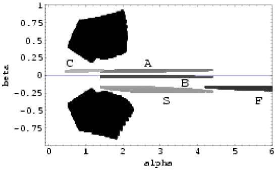
Figure 1: The black region is the experimentally allowed region predicted from a neutrino mass matrix with two zeros of eq. (2.7). The region predicted from the up-quark masses at the GUT scale for five classes $S$, $A$, $B$, $C$ and $F$ in the case I with $h=1.3$.

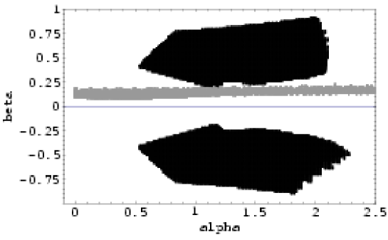
Figure 4: The black region is the experimentally allowed region predicted from a neutrino mass matrix with two zeros of eq. (2.7). The gray region is predicted from the up-quark masses at the GUT scale for the type $C_{1}$ in the case III with $h=1.3$.

which are obtained taking account of RGE’s effect to the quark masses at the EW scale [8]. We have shown that the allowed region of $\alpha$ and $\beta$ given by a neutrino mass matrix with two zeros in eq. (2.7) and the region of $\alpha$ and $\beta$ for the five classes in our model, which are predicted from the up-quark masses at the GUT scale, are slightly separated on the $\alpha$–$\beta$ plane, as seen in Figure 1. However, the light quark masses are ambiguous because of the non-perturbative QCD effect. Therefore, the allowed region of up quark mass, $m_{u}$, may be enlarged . We obtained the overlapped region for the type $S_{1}$ (of the class $S$), as seen in Figure 4 of Ref. [20], enlarging the values of up quark mass at the GUT scale, $m_{u}=0.36\sim 2.56~{}{\rm MeV}$. In the overlapped region, the allowed values of the parameters including the phases are restricted to very narrow regions. On the other hand, our results are almost independent of the phase parameter $\sigma$ and therefore we take $\sigma=0$ in our calculations for simplicity. By taking those values of parameters, we can obtain the prediction of $|U_{e3}|$, $J_{CP}$, $|\langle m_{ee}\rangle|$ and the absolute masses of neutrinos, as shown in the Table 3. In the Table 3, we also list the allowed values for $\sin^{2}\theta_{23}$, $\tan^{2}\theta_{12}$, $\Delta m^{2}_{32}$, $\Delta m^{2}_{32}$, $M_{1}$, $M_{2}$ and $M_{3}$ in the types $S_{1}$ and $S_{2}$. As we can see that, from the Table 3, the difference between the types $S_{1}$ and $S_{2}$ is only the scale of $M_{3}$; the order of $M_{3}$ for $S_{1}$ is larger 1 order than $S_{2}$. For the type $S_{2}$, we obtained the overlapped region, enlarging $m_{u}=0.36\sim 2.64~{}{\rm MeV}$. Therefore, the type $S_{1}$ is the best type in the class $S$.

Type	$\sin^{2}\theta_{23}$	$\tan^{2}\theta_{12}$	$\Delta m^{2}_{32}~{}({\rm{\rm eV}}^{2})$	$\Delta m^{2}_{21}~{}({\rm{\rm eV}}^{2})$	$m_{\nu_{1}}~{}({\rm{\rm eV}})$	$m_{\nu_{2}}~{}({\rm{\rm eV}})$	$m_{\nu_{3}}~{}({\rm{\rm eV}})$	$\phi$
$S_{1}$	$0.42\sim 0.43$	$0.28$	$3.8\times 10{-3}$	$5.4\times 10{-5}$	$0.0014$	$0.0075$	$0.062$	$-\frac{\pi}{18}\sim\frac{\pi}{18}$
$S_{2}$	$0.43$	$0.28$	$3.8\times 10{-3}$	$5.4\times 10{-5}$	$0.0014$	$0.0075$	$0.062$	$0$
Type	$|U_{e3}|$	$J_{{\rm CP}}$		$|\langle M_{ee}\rangle|$	$M_{1}~{}({\rm{\rm GeV}})$	$M_{2}~{}({\rm{\rm GeV}})$	$M_{3}~{}({\rm{\rm GeV}})$	$\rho$
$S_{1}$	$0.010\sim 0.025$	$(-4.8\sim-1.1)\times 10{-3}$		$0.019\sim 0.024$	$1.1\times 10^{9}$	$-1.1\times 10^{9}$	$3.0\times 10^{15}$	$\frac{3\pi}{4}\sim\pi$
$S_{2}$	$0.010$	0		$0.024$	$1.1\times 10^{9}$	$-1.1\times 10^{9}$	$3.5\times 10^{14}$	$\pi$

Table 3: The allowed values for the neutrino observable in the types $S_{1}$ and $S_{2}$. $M_{1}$, $M_{2}$ and $M_{3}$ are the masses for the 1st, 2nd and 3rd generation of the right-handed Majorana neutrino.

In the next section, we will examine whether or not more general form of the right-handed Majorana neutrino mass matrix, which leads to the neutrino mass matrix with two zeros of eq. (2.7), can have parameter regions consistent with the neutrino experimental data, without enlarging the values of up quark mass at the GUT scale.

2.2 Including new parameters in $M_{R}$

2.2.1 Properties for the general form of $M_{R}$

Up to here, we have assumed the simplest form for $M_{R}$, having two parameters,

$${\rm Case~{}I:}\quad M_{R}=\left(\begin{array}[]{@{\,}ccc@{\,}}0&r&0\\ r&0&0\\ 0&0&1\end{array}\right)M_{3}.$$ (2.90)

However, the actual case might have a general form which leads to the neutrino mass matrix with two zeros in eq. (2.7). Thus, we here include the new parameters $s$ and $t$ in $M_{R}$ as follows:

$$M_{R}=\left(\begin{array}[]{@{\,}ccc@{\,}}0&r&0\\ r&s&t\\ 0&t&1\end{array}\right)M_{3},$$ (2.94)

where $r$, $s$ and $t$ are taken to be real. In order to clarify each effect of the new parameters, let us examine the above form, eq. (2.94) by dividing it into the following three cases:

$${\rm Case~{}II:} M_{R}=\left(\begin{array}[]{@{\,}ccc@{\,}}0&r&0\\ r&s&0\\ 0&0&1\end{array}\right)M_{3},$$ (2.98)

$${\rm Case~{}III:} M_{R}=\left(\begin{array}[]{@{\,}ccc@{\,}}0&r&0\\ r&0&t\\ 0&t&1\end{array}\right)M_{3},$$ (2.102)

$${\rm Case~{}IV:} M_{R}=\left(\begin{array}[]{@{\,}ccc@{\,}}0&r&0\\ r&s&t\\ 0&t&1\end{array}\right)M_{3}.$$ (2.106)

The final expression of the left-handed Majorana neutrino mass matrices for each case can be obtained via seesaw mechanism:

$${\rm Case~{}I:} M_{\nu}=\left(\begin{array}[]{@{\,}ccc@{\,}}0&\frac{a^{2}}{r}&0\\ \frac{a^{2}}{r}&\frac{2ab}{r}+c^{2}&\frac{ac}{r}+cd\\ 0&\frac{ac}{r}+cd&d^{2}\end{array}\right)\frac{m_{t}^{2}}{M_{3}},$$ (2.110)

$${\rm Case~{}II:} M_{\nu}=\left(\begin{array}[]{@{\,}ccc@{\,}}0&\frac{a^{2}}{r}&0\\ \frac{a^{2}}{r}&\frac{2ab}{r}-\frac{a^{2}}{r^{2}}s+c^{2}&\frac{ac}{r}+cd\\ 0&\frac{ac}{r}+cd&d^{2}\end{array}\right)\frac{m_{t}^{2}}{M_{3}},$$ (2.114)

$${\rm Case~{}III:} M_{\nu}=\left(\begin{array}[]{@{\,}ccc@{\,}}0&\frac{a^{2}}{r}&0\\ \frac{a^{2}}{r}&\frac{2ab}{r}-\frac{2ac}{r}t+\frac{a^{2}}{r^{2}}t^{2}+c^{2}&\frac{ac}{r}-\frac{ad}{r}t+cd\\ 0&\frac{ac}{r}-\frac{ad}{r}t+cd&d^{2}\end{array}\right)\frac{m_{t}^{2}}{M_{3}},$$ (2.118)

$${\rm Case~{}IV:} M_{\nu}=\left(\begin{array}[]{@{\,}ccc@{\,}}0&\frac{a^{2}}{r}&0\\ \frac{a^{2}}{r}&\frac{2ab}{r}-\frac{a^{2}}{r^{2}}s-\frac{2ac}{r}t+\frac{a^{2}}{r^{2}}t^{2}+c^{2}&\frac{ac}{r}-\frac{ad}{r}t+cd\\ 0&\frac{ac}{r}-\frac{ad}{r}t+cd&d^{2}\end{array}\right)\frac{m_{t}^{2}}{M_{3}}.$$ (2.122)

As is seen from the above expressions, the parameter $s$ affects only on the 2-2 element of $M_{\nu}$, and the additional contribution to the 2-3 element comes only from the parameter $t$. In eqs. (2.110) and (2.114), we found that the 2-3 element of $M_{\nu}$ in the case II is the same as that in the case I, namely, the condition for getting a large mixing angle $\theta_{23}$ in the case II is the same as that in the case I. On the other hand, the condition for the case III is, similarly, the same as that in the case IV. Note that the 1-2 element of $M_{\nu}$ has the same form in all case.

For each case, we will search for the parameter regions, which are allowed by the experimental data within $3\sigma$, and show that, in the case II, the types $S_{1}$ and $S_{2}$ have the allowed regions, the types $C_{1}$, $F_{3}$ and $F_{4}$ in the case III, and the types $S_{1}$, $S_{2}$, $A_{1}$, $B_{1}$, $C_{1}$, $F_{3}$ and $F_{4}$ in the case IV.

2.2.2 Case II

First, let us examine the case II. Since a new parameter, $s$, affects only on the 2-2 element of $M_{\nu}$, namely, $\alpha$, the allowed regions for the classes $S$, $A$, $B$, $C$ and $F$ in the case I, as depicted in Figure 1, can be enlarged only in the direction of $\alpha$. The first term in the 2-2 element becomes comparable with the second term at the following value of $s$:

$$\frac{2ab}{r}\simeq\frac{a^{2}s}{r^{2}}\to s\simeq\frac{2br}{a}\sim\lambda^{9}\sim 5\times 10^{-7}.$$ (2.124)

Thus, the difference between the region of $\alpha$ in the case I and the case II is appreciable around this value of $s$. We obtained the overlapped region in the types $S_{1}$ and $S_{2}$ with $h=1.3$, as depicted in Figure 2 and 3. It is shown that the region which is consistent with the experimental data has now been focused only on the narrow region. The typical values for these types are listed in Table 4, where the values at the maximum and minimum value of $|U_{e3}|$ are written. In this table, as we have expected, we find that the overlapped regions can be obtained around $s\sim 10^{-(6\sim 7)}$. The predicted values of $|U_{e3}|$ is given

$$|U_{e3}|=0.014-0.071,$$ (2.125)

for the type $S_{1}$, and

$$|U_{e3}|=0.013-0.016,$$ (2.126)

for the type $S_{2}$.

Type	$S_{1}^{{\rm max}}$	$S_{1}^{{\rm min}}$	$S_{2}^{{\rm max}}$	$S_{2}^{{\rm min}}$
$|U_{e3}|$	$0.071$	$0.014$	0.016	0.013
$\phi$	0.0	0.0	0.0	0.0
$\rho$	$5\pi/8$	$\pi$	$\pi$	$\pi$
$|\langle M_{ee}\rangle|$	0.022	0.027	0.029	0.027
$J_{{\rm CP}}$	$-0.01$	0.0	0.0	0.0
$m_{\nu_{1}}~{}({\rm eV})$	$1.7\times 10^{-3}$	$1.4\times 10^{-3}$	$1.4\times 10^{-3}$	$1.4\times 10^{-3}$
$m_{\nu_{2}}~{}({\rm eV})$	$7.9\times 10^{-3}$	$7.5\times 10^{-3}$	$7.8\times 10^{-3}$	$7.5\times 10^{-3}$
$m_{\nu_{3}}~{}({\rm eV})$	$5.8\times 10^{-2}$	$5.8\times 10^{-2}$	$5.8\times 10^{-2}$	$5.9\times 10^{-2}$
$\sin^{2}\theta_{23}$	0.45	0.43	0.44	0.43
$\tan^{2}\theta_{12}$	0.29	0.29	0.28	0.28
$\Delta m^{2}_{32}~{}({\rm eV}^{2})$	$3.3\times 10^{-3}$	$3.3\times 10^{-3}$	$3.3\times 10^{-3}$	$3.4\times 10^{-3}$
$\Delta m^{2}_{21}~{}({\rm eV}^{2})$	$6.0\times 10^{-5}$	$5.4\times 10^{-5}$	$5.9\times 10^{-5}$	$5.5\times 10^{-5}$
$m_{u}~{}({\rm MeV})$	0.56	0.52	1.04	1.00
$m_{c}~{}({\rm MeV})$	300	230	300	280
$m_{t}~{}({\rm GeV})$	88	88	108	108
$s$	$1.0\times 10^{-6}$	$6.5\times 10^{-7}$	$7.0\times 10^{-6}$	$6.0\times 10^{-6}$
$M_{1}~{}({\rm GeV})$	$-2.7\times 10^{7}$	$-2.7\times 10^{7}$	$-9.6\times 10^{7}$	$-9.6\times 10^{7}$
$M_{2}~{}({\rm GeV})$	$3.0\times 10^{9}$	$2.0\times 10^{9}$	$3.6\times 10^{9}$	$3.1\times 10^{9}$
$M_{3}~{}({\rm GeV})$	$3.0\times 10^{15}$	$3.0\times 10^{15}$	$5.0\times 10^{14}$	$5.0\times 10^{14}$

Table 4: Results of numerical calculations for $S_{1}$ and $S_{2}$ in the case II. The values at the maximum and minimum value of $|U_{e3}|$ are written.

2.2.3 Case III

Next, we discuss the case III, in which the form of the 2-3 element of $M_{\nu}$ is different from the one in the case I. We have listed the condition for getting a large $\theta_{23}$ of each class in Table 5. Here, a new parameter $t$ is included in the condition of $r$. Therefore, the allowed region for five classes, as seen in Figure 1, can be enlarged both in direction of $\alpha$ and $\beta$. The first term in the 2-3 element becomes comparable with the second term at the following value of $t$:

$$\frac{ac}{r}\simeq\frac{ad}{r}t\to t\simeq\frac{c}{d}\sim\lambda^{4}\sim 2\times 10^{-3}.$$ (2.127)

Thus, the difference between the region of $\alpha$ and $\beta$ in the case I and the case III is appreciable around this value of $t$. We show that the types $C_{1}$, $F_{3}$ and $F_{4}$ provide the overlapped region as depicted in Figure 4, 5 and 6. The typical values of $C_{1}$, $F_{3}$ and $F_{4}$ are listed in Table 6. In similar to the case II, as we have expected, we find that the overlapped regions can be obtained around $t\sim 10^{-3}$. Then, the predicted values of $|U_{e3}|$ is given for the type $C_{1}$,

$$|U_{e3}|\simeq 0.025,$$ (2.128)

for the type $F_{3}$,

$$|U_{e3}|=0.059-0.17,$$ (2.129)

and for the type $F_{4}$,

$$|U_{e3}|\simeq 0.19.$$ (2.130)

The types $C_{1}$ and $F_{4}$ have very narrow region. On the other hand, wide region is obtained in the type $F_{3}$.

Type	condition	Type	condition
$S_{1}$	$r\simeq\frac{-a(c+3t)^{\mathstrut}}{3h+c_{\mathstrut}}$	$S_{2}$	$r\simeq\frac{3a(c-t)}{h-c}$
$A_{1}$	$r\simeq\frac{a(c-t)^{\mathstrut}}{h-c}$	$A_{2}$	$r\simeq\frac{3a(3c+t)}{h+3c}$
$A_{3}$	$r\simeq\frac{a(c+3t)^{\mathstrut}}{3(3h+3c)_{\mathstrut}}$	$A_{4}$	$r\simeq\frac{a(c-t)}{h-c}$
$B_{1}$	$r\simeq\frac{-a(c-t)^{\mathstrut}}{3(h-c)_{\mathstrut}}$	$B_{2}$	$r\simeq\frac{-a(3c+t)}{h+3c}$
$C_{1}$	$r\simeq\frac{a(c-t)^{\mathstrut}}{h-c_{\mathstrut}}$	$C_{2}$	$r\simeq\frac{-a(c-t)}{3(h-c)}$
$C_{3}$	$r\simeq\frac{-a(3c+t)^{\mathstrut}}{h+3c_{\mathstrut}}$	$C_{4}$	$r\simeq\frac{3a(3c+t)}{h+3c}$
$F_{1}$	$r\simeq\frac{-a(c+3t)^{\mathstrut}}{3h+c_{\mathstrut}}$	$F_{2}$	$r\simeq\frac{a(c+3t)}{3(3h+c)}$
$F_{3}$	$r\simeq\frac{a(c-t)^{\mathstrut}}{h-c_{\mathstrut}}$	$F_{4}$	$r\simeq\frac{-3a(c-t)}{h-c}$

Table 5: The condition for getting a large $\theta_{23}$ in the case III and IV.

Type	$C_{1}$	$F_{3}^{{\rm max}}$	$F_{3}^{{\rm min}}$	$F_{4}$
$|U_{e3}|$	0.025	0.17	0.059	0.19
$\phi$	0.0	$-\pi/8$	$\pi/8$	$-\pi/8$
$\rho$	$\pi/8$	$\pi/2$	$\pi/8$	$3\pi/4$
$|\langle M_{ee}\rangle|$	0.019	0.027	0.084	0.57
$J_{{\rm CP}}$	$0.0042$	0.033	$-0.005$	0.031
$m_{\nu_{1}}~{}({\rm eV})$	$1.4\times 10^{-3}$	$3.1\times 10^{-3}$	$1.6\times 10^{-3}$	$5.7\times 10^{-3}$
$m_{\nu_{2}}~{}({\rm eV})$	$7.5\times 10^{-3}$	$9.6\times 10^{-3}$	$8.3\times 10^{-3}$	$9.9\times 10^{-3}$
$m_{\nu_{3}}~{}({\rm eV})$	$6.2\times 10^{-2}$	$4.4\times 10^{-2}$	$3.7\times 10^{-2}$	$4.4\times 10^{-2}$
$\sin^{2}\theta_{23}$	0.46	0.45	0.49	0.30
$\tan^{2}\theta_{12}$	0.28	0.40	0.29	0.56
$\Delta m^{2}_{32}~{}({\rm eV}^{2})$	$3.8\times 10^{-3}$	$1.9\times 10^{-3}$	$1.3\times 10^{-3}$	$1.8\times 10^{-3}$
$\Delta m^{2}_{21}~{}({\rm eV}^{2})$	$5.5\times 10^{-5}$	$8.2\times 10^{-5}$	$6.7\times 10^{-5}$	$6.6\times 10^{-5}$
$m_{u}~{}({\rm MeV})$	0.48	1.2	1.24	1.12
$m_{c}~{}({\rm MeV})$	290	300	220	220
$m_{t}~{}({\rm GeV})$	92	93	88	113
$t$	$1.4\times 10^{-3}$	$3.0\times 10^{-3}$	$3.0\times 10^{-3}$	$2.5\times 10^{-3}$
$M_{1}~{}({\rm GeV})$	$1.2\times 10^{7}$	$4.7\times 10^{5}$	$6.5\times 10^{5}$	$6.2\times 10^{6}$
$M_{2}~{}({\rm GeV})$	$-6.1\times 10^{9}$	$-4.5\times 10^{9}$	$-4.5\times 10^{9}$	$-5.6\times 10^{9}$
$M_{3}~{}({\rm GeV})$	$3.09\times 10^{15}$	$5.0\times 10^{14}$	$5.0\times 10^{14}$	$9.0\times 10^{14}$

Table 6: Results of numerical calculations for $C_{1},F_{3}$ and $F_{4}$ in the case III. The values at the maximum and minimum value of $|U_{e3}|$ are written.

2.2.4 Case IV

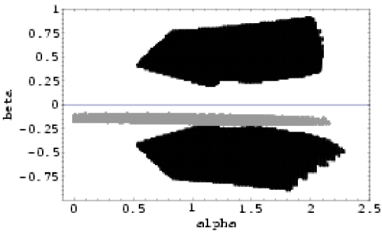
Figure 7: The black region is the experimentally allowed region predicted from a neutrino mass matrix with two zeros of eq. (2.7). The gray region is predicted from the up-quark masses at the GUT scale for the type $S_{1}$ in the case IV with $h=1.3$.

Finally, we consider the most general case for $M_{R}$, which includes two new parameters, $s$ and $t$. In this case, because eq. (2.122) includes both eqs. (2.114) and (2.118), we can expect that $S_{1},S_{2}$, which are allowed in the case II, and $C_{1},F_{3},F_{4}$, which are allowed in the case III, have the overlapped region. By numerical calculations, we have confirmed that $A_{1}$ and $B_{1}$ also provide the overlapped regions as depicted in Figures 7 $\sim$ 13. The typical values of these seven types are listed in Table 7, 8 and 9. We present the predicted values of $|U_{e3}|$ for seven types as follows:

$$|U_{e3}| = 0.014-0.027~{}~{}({\rm Type}~{}S_{1}),$$ (2.131)

$$|U_{e3}| = 0.021-0.19~{}~{}({\rm Type}~{}S_{2}),$$ (2.132)

$$|U_{e3}| = 0.032-0.17~{}~{}({\rm Type}~{}A_{1}),$$ (2.133)

$$|U_{e3}| = 0.049-0.11~{}~{}({\rm Type}~{}B_{1}),$$ (2.134)

$$|U_{e3}| \simeq 0.012~{}~{}({\rm Type}~{}C_{1}),$$ (2.135)

$$|U_{e3}| = 0.056-0.19~{}~{}({\rm Type}~{}F_{3}),$$ (2.136)

$$|U_{e3}| \simeq 0.17~{}~{}({\rm Type}~{}F_{4}).$$ (2.137)

In conclusion, the prediction of $|U_{e3}|$ depends on the types of Dirac neutrino mass matrix and right-handed Majorana mass matrix considerably.

Type	$S_{1}^{{\rm max}}$	$S_{1}^{{\rm min}}$	$S_{2}^{{\rm max}}$	$S_{2}^{{\rm min}}$
$|U_{e3}|$	$0.027$	$0.014$	0.19	0.021
$\phi$	0.0	0.0	$-\pi/8$	0.0
$\rho$	$7\pi/8$	$\pi$	$\pi/4$	0.0
$|\langle M_{ee}\rangle|$	0.024	0.027	0.27	0.034
$J_{{\rm CP}}$	$-4.0\times 10^{-3}$	0.0	0.034	0.0
$m_{\nu_{1}}~{}({\rm eV})$	$1.5\times 10^{-3}$	$1.4\times 10^{-3}$	$4.3\times 10^{-3}$	$1.7\times 10^{-3}$
$m_{\nu_{2}}~{}({\rm eV})$	$7.6\times 10^{-3}$	$7.6\times 10^{-3}$	$9.1\times 10^{-3}$	$7.5\times 10^{-3}$
$m_{\nu_{3}}~{}({\rm eV})$	$5.8\times 10^{-2}$	$5.8\times 10^{-2}$	$5.0\times 10^{-2}$	$5.9\times 10^{-2}$
$\sin^{2}\theta_{23}$	0.44	0.43	0.38	0.46
$\tan^{2}\theta_{12}$	0.29	0.28	0.39	0.35
$\Delta m^{2}_{32}~{}({\rm eV}^{2})$	$3.3\times 10^{-3}$	$3.3\times 10^{-3}$	$2.4\times 10^{-3}$	$3.4\times 10^{-3}$
$\Delta m^{2}_{21}~{}({\rm eV}^{2})$	$5.5\times 10^{-5}$	$5.5\times 10^{-5}$	$6.4\times 10^{-5}$	$5.4\times 10^{-5}$
$m_{u}~{}({\rm MeV})$	1.28	0.52	0.96	0.48
$m_{c}~{}({\rm MeV})$	280	290	270	280
$m_{t}~{}({\rm GeV})$	88	88	93	108
$s$	$1.0\times 10^{-6}$	$1.0\times 10^{-6}$	$8.0\times 10^{-6}$	$6.0\times 10^{-6}$
$t$	$1.0\times 10^{-4}$	$1.0\times 10^{-4}$	$2.0\times 10^{-3}$	$4.0\times 10^{-3}$
$M_{1}~{}({\rm GeV})$	$-1.5\times 10^{8}$	$-2.9\times 10^{7}$	$-2.9\times 10^{7}$	$1.1\times 10^{7}$
$M_{2}~{}({\rm GeV})$	$3.1\times 10^{9}$	$3.0\times 10^{9}$	$2.0\times 10^{9}$	$-5.0\times 10^{9}$
$M_{3}~{}({\rm GeV})$	$3.0\times 10^{15}$	$3.0\times 10^{15}$	$5.0\times 10^{14}$	$5.0\times 10^{14}$

Table 7: Results of numerical calculations for $S_{1}$ and $S_{2}$ in the case IV. The values at the maximum and minimum value of $|U_{e3}|$ are written.

Type	$A_{1}^{{\rm max}}$	$A_{1}^{{\rm min}}$	$B_{1}^{{\rm max}}$	$B_{1}^{{\rm min}}$
$|U_{e3}|$	$0.17$	$0.032$	0.11	0.049
$\phi$	0.0	0.0	0.0	0.0
$\rho$	$\pi$	0.0	$\pi/2$	0.0
$|\langle M_{ee}\rangle|$	0.24	0.049	0.096	0.075
$J_{{\rm CP}}$	$-0.01$	0.0	0.012	0.0
$m_{\nu_{1}}~{}({\rm eV})$	$3.6\times 10^{-3}$	$1.6\times 10^{-3}$	$1.9\times 10^{-3}$	$1.9\times 10^{-3}$
$m_{\nu_{2}}~{}({\rm eV})$	$8.6\times 10^{-3}$	$8.4\times 10^{-3}$	$8.5\times 10^{-3}$	$8.5\times 10^{-3}$
$m_{\nu_{3}}~{}({\rm eV})$	$6.0\times 10^{-2}$	$5.1\times 10^{-2}$	$4.7\times 10^{-2}$	$4.7\times 10^{-2}$
$\sin^{2}\theta_{23}$	0.42	0.48	0.48	0.49
$\tan^{2}\theta_{12}$	0.40	0.31	0.29	0.37
$\Delta m^{2}_{32}~{}({\rm eV}^{2})$	$3.5\times 10^{-3}$	$2.6\times 10^{-3}$	$2.1\times 10^{-3}$	$2.1\times 10^{-3}$
$\Delta m^{2}_{21}~{}({\rm eV}^{2})$	$6.2\times 10^{-5}$	$6.7\times 10^{-5}$	$6.8\times 10^{-5}$	$6.8\times 10^{-5}$
$m_{u}~{}({\rm MeV})$	0.36	0.44	0.8	0.8
$m_{c}~{}({\rm MeV})$	210	260	300	300
$m_{t}~{}({\rm GeV})$	113	108	103	103
$s$	$3.0\times 10^{-6}$	$4.0\times 10^{-6}$	$8.0\times 10^{-6}$	$8.0\times 10^{-6}$
$t$	$1.5\times 10^{-3}$	$1.5\times 10^{-3}$	$3.0\times 10^{-3}$	$3.0\times 10^{-3}$
$M_{1}~{}({\rm GeV})$	$-1.9\times 10^{6}$	$-4.4\times 10^{6}$	$3.5\times 10^{5}$	$3.5\times 10^{5}$
$M_{2}~{}({\rm GeV})$	$3.8\times 10^{9}$	$8.8\times 10^{9}$	$-5.0\times 10^{9}$	$-5.0\times 10^{9}$
$M_{3}~{}({\rm GeV})$	$5.0\times 10^{15}$	$5.0\times 10^{15}$	$5.0\times 10^{15}$	$5.0\times 10^{15}$

Table 8: Results of numerical calculations for $A_{1}$ and $B_{1}$ in the case IV. The values at the maximum and minimum value of $|U_{e3}|$ are written.

Type	$C_{1}$	$F_{3}^{{\rm max}}$	$F_{3}^{{\rm min}}$	$F_{4}^{{\rm max}}$	$F_{4}^{{\rm min}}$
$|U_{e3}|$	0.012	0.19	0.056	0.19	0.17
$\phi$	0.0	$-\pi/8$	0.0	0.0	$-\pi/8$
$\rho$	0.0	$3\pi/4$	0.0	$\pi$	$7\pi/8$
$|\langle M_{ee}\rangle|$	0.025	0.35	0.089	0.67	0.51
$J_{{\rm CP}}$	0.0	0.034	0.0	0.0	0.031
$m_{\nu_{1}}~{}({\rm eV})$	$1.4\times 10^{-3}$	$2.9\times 10^{-3}$	$1.6\times 10^{-3}$	$5.5\times 10^{-3}$	$5.6\times 10^{-3}$
$m_{\nu_{2}}~{}({\rm eV})$	$7.5\times 10^{-3}$	$8.6\times 10^{-3}$	$7.5\times 10^{-3}$	$1.1\times 10^{-2}$	$9.9\times 10^{-3}$
$m_{\nu_{3}}~{}({\rm eV})$	$6.1\times 10^{-2}$	$4.0\times 10^{-2}$	$3.7\times 10^{-2}$	$3.9\times 10^{-2}$	$4.8\times 10^{-2}$
$\sin^{2}\theta_{23}$	0.46	0.44	0.50	0.39	0.30
$\tan^{2}\theta_{12}$	0.28	0.35	0.35	0.56	0.59
$\Delta m^{2}_{32}~{}({\rm eV}^{2})$	$3.7\times 10^{-3}$	$1.5\times 10^{-3}$	$1.3\times 10^{-3}$	$1.4\times 10^{-3}$	$2.2\times 10^{-3}$
$\Delta m^{2}_{21}~{}({\rm eV}^{2})$	$5.5\times 10^{-5}$	$6.6\times 10^{-5}$	$5.4\times 10^{-5}$	$9.4\times 10^{-5}$	$6.7\times 10^{-5}$
$m_{u}~{}({\rm MeV})$	0.88	1.12	1.24	1.12	1.2
$m_{c}~{}({\rm MeV})$	300	290	210	210	210
$m_{t}~{}({\rm GeV})$	88	88	88	113	118
$s$	$3.2\times 10^{-7}$	$2.0\times 10^{-7}$	$4.0\times 10^{-7}$	$4.0\times 10^{-7}$	$1.0\times 10^{-7}$
$t$	$1.9\times 10^{-3}$	$3.0\times 10^{-3}$	$3.0\times 10^{-3}$	$2.5\times 10^{-3}$	$2.5\times 10^{-3}$
$M_{1}~{}({\rm GeV})$	$2.8\times 10^{7}$	$4.5\times 10^{5}$	$6.5\times 10^{5}$	$6.3\times 10^{6}$	$6.7\times 10^{6}$
$M_{2}~{}({\rm GeV})$	$-9.4\times 10^{9}$	$-4.4\times 10^{9}$	$-4.3\times 10^{9}$	$-5.3\times 10^{9}$	$-5.5\times 10^{9}$
$M_{3}~{}({\rm GeV})$	$2.85\times 10^{15}$	$5.0\times 10^{14}$	$5.0\times 10^{14}$	$9.0\times 10^{14}$	$9.0\times 10^{14}$

Table 9: Results of numerical calculations for $C_{1},F_{3}$ and $F_{4}$ in the case IV. The values at the maximum and minimum value of $|U_{e3}|$ are written.

3 Lepton flavor violations : $e_{j}\rightarrow e_{i}\gamma$

In the model of MSSM with right-handed neutrinos, lepton flavor violations (LFV) are induced through the renormalization group effects to the slepton mixings and the predicted branching ratios of the processes can be comparable with the current experimental upper bound [24, 25, 26, 27, 28, 29, 30] :

$${\rm Br}(\mu\rightarrow e\gamma) < 1.2\times 10^{-11}\ \cite[cite]{[\@@bibref{}{exp-muegam}{}{}]}\ ,$$ (3.1)

$${\rm Br}(\tau\rightarrow e\gamma) < 3.6\times 10^{-7}\ \cite[cite]{[\@@bibref{}{Hisano}{}{}]}\ ,$$ (3.2)

$${\rm Br}(\tau\rightarrow\mu\gamma) < 3.1\times 10^{-7}\ \cite[cite]{[\@@bibref{}{Belle-taumugam}{}{}]}\ .$$ (3.3)

Therefore, we have to examine these decay rates carefully in our model.

Let us start with writing down the leptonic parts of soft SUSY breaking terms as follows:

$$-{\cal{L}}_{\rm soft}=(m_{\tilde{L}}^{2})_{ij}{\tilde{L}}_{i}^{\dagger}{\tilde{L}}_{j}+(m_{\tilde{e}}^{2})_{ij}{\tilde{e}}_{Ri}^{*}{\tilde{e}}_{Rj}+(m_{\tilde{\nu}}^{2})_{ij}{\tilde{\nu}}_{Ri}^{*}{\tilde{\nu}}_{Rj}+(A_{e})_{ij}H_{d}{\tilde{e}}_{Ri}^{*}{\tilde{L}}_{j}+(A_{\nu})_{ij}H_{u}{\tilde{\nu}}_{Ri}^{*}{\tilde{L}}_{j}\ ,$$ (3.4)

where ${\tilde{L}}_{i},{\tilde{e}}_{Ri}$ and ${\tilde{\nu}}_{Ri}$ are the supersymmetric scalar partner of left-handed lepton doublet, right-handed lepton singlet and right-handed neutrino, $(m_{\tilde{L}}^{2})_{ij},(m_{\tilde{e}}^{2})_{ij}$ and $(m_{\tilde{\nu}}^{2})_{ij}$ are the $3\times 3$ hermitian slepton mass matrices, $(A_{e})_{ij}$ and $(A_{\nu})_{ij}$ are trilinear couplings of Higgs doublets $H_{u},H_{d}$ and sleptons, respectively (A-term). $H_{u}$ and $H_{d}$ couple to neutrinos and charged leptons, respectively. Non-vanishing off-diagonal elements of slepton mass matrices become the new source of LFV.

In minimal-supergravity (mSUGRA) models, it is assumed that the slepton mass matrices are diagonal and have common mass scale $m_{0}$ at the GUT scale, and that the trilinear couplings are proportional to Yukawa couplings:

$$(m_{\tilde{L}}^{2})_{ij}=(m_{\tilde{e}}^{2})_{ij}=(m_{\tilde{\nu}}^{2})_{ij}=\delta_{ij}m_{0}^{2}\ ,\ \ m_{H_{d}}^{2}=m_{H_{u}}^{2}=m_{0}^{2}\ ,$$

$$A_{\nu}=Y_{\nu}a_{0}m_{0}\ ,\ \ A_{e}=Y_{e}a_{0}m_{0}\ ,$$ (3.5)

and the same conditions are assumed in quark sector. The mass of supersymmetric fermion partner of gauge bosons (gauginos) are also fixed to be $M_{1/2}$ at the GUT scale. Even if no sources of LFV are assumed at the GUT scale, the LFV will be induced in slepton mass matrix through renormalization of Yukawa and gauge interactions. The one-loop renormalization group equation (RGE) for left-handed slepton mass matrix is given by

$$\mu\frac{d}{d\mu}(m_{\tilde{L}}^{2})_{ij}=\left.\mu\frac{d}{d\mu}(m_{\tilde{L}}^{2})_{ij}\right|_{\rm MSSM}\hskip 256.0748pt$$

$$+\frac{1}{16\pi^{2}}\left[(m_{\tilde{L}}^{2}Y_{\nu}^{\dagger}Y_{\nu}+Y_{\nu}^{\dagger}Y_{\nu}m_{\tilde{L}}^{2})_{ij}+2(Y_{\nu}^{\dagger}m_{\tilde{\nu}}Y_{\nu}+m_{H_{u}}^{2}Y_{\nu}^{\dagger}Y_{\nu}+A_{\nu}^{\dagger}A_{\nu})_{ij}\right]\ ,$$ (3.6)

where the first term is the MSSM term which is lepton flavor conserving, while the second term contains the source of LFV, $Y_{\nu}$ is the neutrino Yukawa coupling matrix ($=M_{\nu_{D}}/v_{u}$).

It is easy to see in eq. (3.6) that the Yukawa coupling of the neutrino contributes to the LFV. Assuming the boundary conditions of eq. (3.5), we obtain the leading log approximation for the off-diagonal elements of left-handed slepton mass matrix at the scale of right-handed neutrino masses as follows [25, 26, 30]:

$$(m_{\tilde{L}}^{2})_{ij}\simeq-\frac{1}{8\pi}(3m_{0}^{2}+a_{0}^{2})H_{ij}\ ,$$ (3.7)

where the matrix $H_{ij}$ is defined by

$$H_{ij}\equiv(\overline{Y_{\nu}}^{{\dagger}}L\overline{Y_{\nu}})_{ij}\ ,\ \ L\equiv diag\left(\ln\frac{M_{\rm GUT}}{M_{1}},\ln\frac{M_{\rm GUT}}{M_{2}},\ln\frac{M_{\rm GUT}}{M_{3}}\right)\ ,$$ (3.8)

where $\overline{Y_{\nu}}$ is the neutrino Yukawa coupling matrix on the basis where the charged lepton and right-handed Majorana mass matrix is diagonal. The branching ratio for the LFV processes: $e_{j}\rightarrow e_{i}\gamma$ is approximately given by

$${\rm Br}(e_{j}\rightarrow e_{i}\gamma)\simeq\frac{\alpha^{3}}{G_{\rm F}^{2}}\,\frac{|(m_{\tilde{L}}^{2})_{ij}|^{2}}{m_{S}^{8}}\,\tan^{2}\!\beta_{v}\ ,$$ (3.9)

where $m_{S}$ is the typical mass scale of superparticles, $\alpha\simeq 1/128$ and $G_{\rm F}$ is the Fermi coupling constant, respectively. The excellent approximation of $m_{S}$ to the exact RGE result is given by [34]

$$m_{S}^{8}\simeq 0.5\,m_{0}^{2}M_{1/2}^{2}(m_{0}^{2}+0.6M_{1/2}^{2})^{2}\ .$$ (3.10)

It is clear that the element $H_{12}$, $H_{13}$ and $H_{23}$ dominantly contribute to the processes of $\mu\rightarrow e\gamma$, $\tau\rightarrow e\gamma$ and $\tau\rightarrow\mu\gamma$, respectively.

Let us calculate the matrix $H_{ij}$ in our model. The $\overline{Y_{\nu}}$ is given by

$$\overline{Y_{\nu}}=O_{R}Y_{\nu}O_{l}\ ,$$ (3.11)

where matrix $O_{R}$ and $O_{l}$ are the orthogonal matrices which diagonalize the right-handed Majorana mass matrix and charged lepton mass matrix, respectively. Then, the matrix $H_{ij}$ is given by

$$H_{ij} = (O_{l}^{T}Y_{\nu}^{{\dagger}}O_{R}^{T})_{ik}L_{k}(O_{R}Y_{\nu}O_{l})_{kj}\ .$$ (3.12)

For the case I, matrix $O_{R}$ is given by

$$O_{R}=\left(\begin{array}[]{ccc}1/\sqrt{2}&1/\sqrt{2}&0\\ -1/\sqrt{2}&1/\sqrt{2}&0\\ 0&0&1\end{array}\right)\ ,$$ (3.16)

then we obtain the formulae of $H_{ij}$ assuming the type $S_{1}$ for neutrino Yukawa coupling matrix which is the mostly allowed one :

$$H_{12} \simeq \left[a^{2}\left(O_{l11}O_{l12}+O_{l21}O_{l22}\right)+\left(bO_{l21}+cO_{l31}\right)\left(bO_{l22}+cO_{l32}\right)\right.$$ (3.17)

$$\left.a\left\{b(O_{l13}O_{l21}+O_{l11}O_{l22})+c(O_{l12}O_{l31}+O_{l11}O_{l32})\right\}\right]\ln\frac{M_{\rm GUT}}{M_{1}}$$

$$+(cO_{l12}+dO_{l31})(cO_{l22}+dO_{l32})\ln\frac{M_{\rm GUT}}{M_{3}}\ ,$$

$$H_{13} \simeq \left[a^{2}\left(O_{l11}O_{l13}+O_{l21}O_{l23}\right)+\left(bO_{21}+cO_{l31}\right)\left(bO_{l23}+cO_{l33}\right)\right.$$ (3.18)

$$\left.a\left\{b(O_{l13}O_{l21}+O_{l11}O_{l23})+c(O_{l13}O_{l31}+O_{l11}O_{l33})\right\}\right]\ln\frac{M_{\rm GUT}}{M_{1}}$$

$$+(cO_{l21}+dO_{l31})(cO_{l23}+dO_{l33})\ln\frac{M_{\rm GUT}}{M_{3}}\ ,$$

$$H_{23} \simeq \left[a^{2}\left(O_{l12}O_{l13}+O_{l22}O_{l23}\right)+\left(bO_{l22}+cO_{l32}\right)\left(bO_{l23}+cO_{l33}\right)\right.$$ (3.19)

$$\left.a\left\{b(O_{l13}O_{l22}+O_{l12}O_{l23})+c(O_{l13}O_{l32}+O_{l12}O_{l33})\right\}\right]\ln\frac{M_{\rm GUT}}{M_{1}}$$

$$+(cO_{l22}+dO_{l32})(cO_{l23}+dO_{l33})\ln\frac{M_{\rm GUT}}{M_{3}}\ ,$$

where we have used the mass spectrum for the case I : $M_{1}=M_{2}$. In the following calculations of branching ratios, the relations : $a=-3a_{u},b=b_{u},c=c_{u},d=-3d_{u}$ for the type $S_{1}$ and $a=-3a_{u},b=b_{u},c=c_{u},d=d_{u}$ for the type $S_{2}$ will be taken. The orthogonal matrix $O_{l}$ is approximately given by [18]

$$O_{l}\simeq\left(\begin{array}[]{ccc}1&\sqrt{\frac{m_{e}}{m_{\mu}}}&\sqrt{\frac{m_{e}^{2}m_{\mu}}{m_{\tau}^{3}}}\\ -\sqrt{\frac{m_{e}}{m_{\mu}}}&1&\sqrt{\frac{m_{e}}{m_{\tau}}}\\ \sqrt{\frac{m_{e}^{2}}{m_{\mu}m_{\tau}}}&-\sqrt{\frac{m_{e}}{m_{\tau}}}&1\end{array}\right)=\left(\begin{array}[]{ccc}1&\varepsilon&\varepsilon\delta^{2}\\ -\varepsilon&1&\delta\\ \varepsilon\delta&-\delta&1\end{array}\right)\ ,\ \ \varepsilon\equiv\sqrt{\frac{m_{e}}{m_{\mu}}}\ ,\ \delta\equiv\sqrt{\frac{m_{e}}{m_{\tau}}}\ .$$ (3.26)

Under the above parameterization, we can calculate the off-diagonal elements of matrix $H_{ij}$ :

$$|H_{12}|\simeq\left|ab\ln\frac{M_{\rm GUT}}{M_{1}}-b^{2}\varepsilon\ln\frac{M_{\rm GUT}}{M_{1}}-d^{2}\delta^{2}\varepsilon\ln\frac{M_{\rm GUT}}{M_{3}}\right|\simeq d^{2}\delta^{2}\varepsilon\ln\frac{M_{\rm GUT}}{M_{3}}\ ,$$ (3.27)

$$|H_{13}|\simeq\left|ac\ln\frac{M_{\rm GUT}}{M_{1}}-bc\varepsilon\ln\frac{M_{\rm GUT}}{M_{1}}+d^{2}\delta\varepsilon\ln\frac{M_{\rm GUT}}{M_{3}}\right|\simeq d^{2}\delta\varepsilon\ln\frac{M_{\rm GUT}}{M_{3}}\ ,$$ (3.28)

$$|H_{23}|\simeq\left|cd\ln\frac{M_{\rm GUT}}{M_{3}}-c^{2}\delta\ln\frac{M_{\rm GUT}}{M_{1}}+d^{2}\delta\ln\frac{M_{\rm GUT}}{M_{3}}\right|\simeq d^{2}\delta\ln\frac{M_{\rm GUT}}{M_{3}}\ ,$$ (3.29)

where the terms including the charged lepton mixing matrix are dominant ones. These formulae provide the following relations of branching ratios :

$${\rm Br}(\mu\rightarrow e\gamma)<{\rm Br}(\tau\rightarrow e\gamma)<{\rm Br}(\tau\rightarrow\mu\gamma)\ ,$$ (3.30)

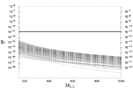
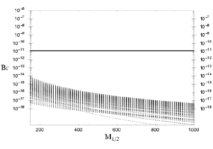
Figure 14: The predicted branching ratio of $\mu\rightarrow e\gamma$ process as a function of $M_{1/2}$ (GeV) taking $a_{0}=0$, $m_{0}=100\sim 1000\,{\rm GeV}$ for $\tan\beta=5\sim 50$ are shown. The left and right figure correspond to the type $S_{1}$ and $S_{2}$, respectively. The horizontal line is experimental upper bound.

for the type $S_{1}$ and $S_{2}$. For the case II, III and IV, the predicted branching ratios are almost the same as the case I. Numerical calculations of the branching ratios using the leading log approximation (eps. (3.7), (3.8), (3.9) and (3.10)) of $\mu\rightarrow e\gamma$, $\tau\rightarrow e\gamma$ and $\tau\rightarrow\mu\gamma$ are presented in Figure 14, 15 and 16, respectively . In these figures, the branching ratios are scatter plotted in the region of $m_{0}=100\sim 1000~{}{\rm GeV}$, $M_{1/2}=100\sim 1000~{}{\rm GeV}$ and $\tan\beta=5\sim 50$ for each processes. The $a_{0}$ is fixed to be $a_{0}=0$.

As seen in these figures, the branching ratios of all processes are safely predicted below the current experimental upper bounds. The predicted branching ratios for the type $S_{2}$ are lower almost one order of magnitude than the one for the type $S_{1}$. This is due to the differences in CG coefficients in 3-3 elements of neutrino Yukawa coupling matrix. Only $\tau\rightarrow\mu\gamma$ process for the type $S_{1}$ may be observed in the future experiments in which the sensitivity will reach to be ${\rm Br}(\tau\rightarrow\mu\gamma)\leq 10^{-9}$ [35]. The predicted branching ratios of $\tau\rightarrow\mu\gamma$ process for the type $S_{2}$ and the other processes for both types are too small to be observed even in the future experiments.

4 Thermal Leptogenesis

In this section, we discuss the calculation of baryon asymmetry of the universe based on the leptogenesis scenario [36] for our textures. In the leptogenesis scenario, lepton asymmetry is generated by the CP violating out-of-equilibrium decay of heavy right-handed Majorana neutrinos. Let us consider the CP asymmetry parameter $\epsilon_{1}$, which is generated in the decay of $i$-th generation of right-handed Majorana neutrino $N_{i}$. The $\epsilon_{i}$ is defined as

$$\epsilon_{i}\equiv\frac{\Gamma(N_{i}\rightarrow H\,L)-\Gamma(N_{i}\rightarrow\overline{H}\,\overline{L})}{\Gamma(N_{i}\rightarrow H\,L)+\Gamma(N_{i}\rightarrow\overline{H}\,\overline{L})}\ ,$$ (4.1)

where $H$ and $L$ are the ordinary Higgs and lepton doublet. At tree level, the decay width of $N_{i}$ can be easily calculated as :

$$\Gamma_{i}^{0}=\frac{(Y_{\nu}Y_{\nu}^{{\dagger}})_{ii}}{8\pi}M_{i}\ .$$ (4.2)

As seen in (4.2), even if the Yukawa coupling matrix $Y_{\nu}$ contains complex elements, CP symmetry is not violated at tree level. Therefore, we should consider the one-loop contributions. It is well-known that CP is violated in the interference between the tree diagram and one-loop self-energy and vertex correction diagrams. Summing up the one-loop vertex and self-energy corrections, the CP asymmetry is given by

$$\epsilon_{i}=\epsilon^{V}_{i}+\epsilon^{S}_{i}=-\frac{1}{8\pi}\frac{1}{(Y_{\nu}Y_{\nu}^{{\dagger}})_{ii}}\sum_{j\neq i}{\rm Im}[(Y_{\nu}Y_{\nu}^{{\dagger}})_{ij}^{2}]\left[v\left(x\right)+s\left(x\right)\right]\ ,$$ (4.3)

where $v(x)$ and $s(x)$ are the self-energy and vertex correction functions with $x\equiv M_{j}^{2}/M_{i}^{2}$ [37]. In the minimal supersymmetric standard model (MSSM) with right-handed neutrinos, they are given by [37, 38]

$$v(x)=\sqrt{x}\ \ln\left(\frac{1+x}{x}\right)\ ,\ \ \ s(x)\equiv\frac{(M_{j}^{2}-M_{i}^{2})M_{i}M_{j}}{(M_{j}^{2}-M_{i}^{2})^{2}+M_{i}^{2}(\Gamma^{0}_{j})^{2}}=\frac{(x-1)\sqrt{x}}{(x-1)^{2}+(\Gamma^{0}_{j})^{2}/M_{i}^{2}}\ ,$$ (4.4)

which is available for both cases of the hierarchical case and the quasi-degenerate case of $M_{i}$ and $M_{j}$.

In order to calculate the baryon asymmetry, we need to solve the Boltzmann equations in thermal leptogenesis scenario [39]. We can use the approximate solution of these Boltzmann equations as

$$\eta_{B}\simeq 0.01\,\sum_{i}\epsilon_{i}\kappa_{i}\ ,$$ (4.5)

where $\eta_{B}$ is baryon asymmetry of the universe, $\kappa_{i}$ is so-called dilution factor which describe the wash-out effect of generated lepton asymmetry. The $\kappa_{i}$ is approximated as [40]

$$\kappa_{i}\simeq 0.3\left(\frac{10^{-3}_{,}{\rm eV}}{\tilde{m}_{i}}\right)\left(\ln\frac{\tilde{m}_{i}}{10^{-3}_{,}{\rm eV}}\right)^{-0.6}\ ,\ \ \tilde{m}_{i}\equiv\frac{(M_{\nu D}M_{\nu D}^{{\dagger}})_{ii}}{M_{i}}\ .$$ (4.6)

In the following, we compare the current range of observed baryon asymmetry [41] :

$$\eta_{B}=(6.2-6.9)\times 10^{-10}\ .$$ (4.7)

with the predicted values of our model.

It is convenient to discuss the hierarchical case : $M_{1}\ll M_{2},M_{3}$ and degenerate case : $M_{1}\simeq M_{2}\ll M_{3}$ of right-handed Majorana masses, separately. For the hierarchical case, from the model independent analyses of thermal leptogenesis [42, 43], the lightest Majorana neutrino mass must satisfy the condition :

$$M_{1}>4.9\times 10^{8}\ {\rm GeV}\ ,$$ (4.8)

to generate the observed baryon asymmetry of the universe. The case II, III and IV correspond to the hierarchical case. In these cases, as shown in the numerical results of tables, the lightest Majorana neutrino mass $M_{1}$ is lighter than $4.9\times 10^{8}\,{\rm GeV}$ for all types to satisfy the conditions of the current neutrino experiments. Therefore, it is impossible to explain the observed baryon asymmetry by thermal leptogenesis for the case of II, III and IV.

On the other hand, the case I corresponds to the degenerate case : $M_{1}\simeq M_{2}\ll M_{3}$. This case satisfies the relation : $M_{2}-M_{1}\leq\Gamma_{1}+\Gamma_{2}$. It is easy to find in eqs. (4.4) that there occurs an enhancement of CP asymmetry for some region of the degeneracy and $\epsilon_{i}=0$ for the case of exact degeneracy : $M_{1}=M_{2}$. The scenario utilizing this enhancement is called as “resonant leptogenesis” [44, 45]. Some author showed that observed baryon asymmetry can be generated with considerably light right-handed neutrino masses, in complete accordance with the current solar and atmospheric neutrino experiments [45, 46, 47, 48, 49, 50, 51, 52]. This is a candidate to solve the gravitino problem [53].

The mass eigenvalues of right-handed Majorana neutrinos for the case I are exactly degenerate : $M_{1}=M_{2}=rM_{3}\simeq 10^{9}~{}{\rm GeV}$. However, it is natural to explain that the mass spectrum may be somewhat deviated from exact degeneracy by, for example, quantum corrections. Let us define the degree of degeneracy for $M_{1}$ and $M_{2}$ by

$$\Delta M\equiv\frac{M_{2}}{M_{1}}-1\ .$$ (4.9)

The predicted baryon asymmetry is shown in Figure 17 as a function of $\Delta M$. As seen in Figure 17, if the degree of degeneracy is the level of $\Delta M\simeq 10^{-3}$, the predicted asymmetry is consistent with the observed value for the type $S_{1}$ in the case I. It is concluded that the baryon asymmetry can be explained by the resonant leptogenesis scenario in the suitable region of the mass degeneracy in our model. Almost the same result is obtained for the type $S_{2}$.

5 Summary

We have investigated the symmetric 2-zero texture of neutrino mass matrix for the possible four textures of the right-handed Majorana neutrino together with the Dirac neutrino mass matrix with two zeros, under the SUSY $SO(10)$ GUT model including the Pati-Salam symmetry. We made a full analysis for the parameters included in such four cases of neutrino mass matrices and showed how they are consistently explain the neutrino masses and mixing angles as well as the baryon number in the Universe via leptogenesis.

In the case I, which has the simplest form of right-handed Majorana neutrino mass matrix with two parameters as seen in eq. (2.90), the class $S$ is consistent with the current neutrino experimental data, if we are allowed to take a little larger value of up quark mass at the GUT scale. On the contrary, in the other three cases which are slightly extended to more general cases within 2-zero texture, having one or two new parameters as seen in eq. (2.98), (2.102) and (2.106), it is shown that the type $S_{1}$ and $S_{2}$ have the experimentally allowed regions in the case II, the types $C_{1}$, $F_{3}$ and $F_{4}$ in the case III, and the types $S_{1}$, $S_{2}$, $A_{1}$, $B_{1}$, $C_{1}$, $F_{3}$ and $F_{4}$ in the case IV. We found that the prediction of $|U_{e3}|$ depends on the types of Dirac neutrino and right-handed Majorana mass matrix, considerably.

We have also calculated the branching ratios of LFV processes for the type $S_{1}$ and $S_{2}$. The predicted branching ratios are well below the experimental upper bounds except $\tau\rightarrow\mu\gamma$ process for the case $S_{1}$. On the other hand, for the case II, III and IV, the predicted branching ratios are almost same as the case I. Also, we have discussed the thermal leptogenesis in our model. Because in the case II, III and IV corresponding to the hierarchical case, the lightest Majorana neutrino mass $M_{1}$ is lighter than $4.9\times 10^{8}\,{\rm GeV}$ for all types to satisfy the conditions of the current neutrino experiments, it is impossible to explain the observed baryon asymmetry by thermal leptogenesis for the case of II, III and IV.

In summary, we have shown that only the class $S$ in the case I, having degenerate mass spectrum for the 1st and 2nd generation of right-handed Majorana neutrino, can simultaneously explain the current neutrino experimental data, lepton flavor violating process and baryon asymmetry of the Universe. The precision measurements for neutrino mixings and mass-squared differences, furthermore, LFV will test if such model is realized in Nature in near future.

Appendix A Phases in neutrino mass matrices

The complex symmetric matrices are given for the Dirac and Majorana neutrinos as follows:

$$M_{\nu D}=\left(\matrix{0&a&0\cr a&b&c\cr 0&c&d}\right)m_{t}\ ,\qquad M_{R}=\left(\matrix{0&r&0\cr r&0&0\cr 0&0&1}\right)M_{3}\ ,$$ (A.1)

where each element is complex in general except for $M_{3}$ and $m_{t}$. The matrix $M_{R}$ is transformed to the real symmetric matrix by phase matrix $P_{R}$

$$M_{R}\rightarrow\quad\overline{M}_{R}=P_{R}^{*}M_{R}P_{R}^{*}=\left(\matrix{0&|r|&0\cr|r|&0&0\cr 0&0&1}\right)M_{3}\ ,\qquad P_{R}=\left(\matrix{e^{-i\tau}&0&0\cr 0&e^{i(\tau+\chi)}&0\cr 0&0&1}\right)\ ,$$ (A.2)

where $\chi=\arg[r]$.

On the other hand, the Dirac neutrino mass matrix turns to

$$M_{\nu D}\rightarrow\quad\widehat{M}_{\nu D}=P_{R}^{*}M_{\nu D}P=\left(\matrix{0&|a|&0\cr|a|&|b|e^{i\phi_{1}}&|c|\cr 0&|c|&|d|e^{i\phi_{2}}}\right)m_{t}\ ,\quad P=\left(\matrix{e^{i\alpha_{\nu}}&0&0\cr 0&e^{i\beta_{\nu}}&0\cr 0&0&e^{i\gamma_{\nu}}}\right)\ ,$$ (A.3)

where

$$\alpha_{\nu}=\chi-2\arg[a]+\arg[c]\ ,\hskip 62.59596pt\beta_{\nu}=-\arg[c]\ ,$$

$$\gamma_{\nu}=\chi-\arg[a]\ ,\hskip 116.65646pt\tau=\arg[c]-\arg[a]\ ,$$

$$\phi_{1}=\arg[a]+\arg[b]-2\arg[c]+\chi\ ,\qquad\phi_{2}=-\arg[a]+\arg[d]+\chi\ .$$ (A.4)

By using the seesaw formula, we have neutrino mass matrix

$$M_{\nu}=M_{\nu_{D}}^{T}M_{R}^{-1}M_{\nu_{D}}=P^{*}\widehat{M}_{\nu}P^{*}$$ (A.5)

where

$$\widehat{M}_{\nu} = \widehat{M}_{\nu D}^{T}\ \overline{M}_{R}^{-1}\ \widehat{M}_{\nu D}$$ (A.6)

$$= \left(\matrix{0&|a|^{2}&0\cr|a|^{2}&|r||c|^{2}+2|a||b|e^{i\phi_{1}}&|a||c|+|r||c||d|e^{i\phi_{2}}\cr 0&|a||c|+|r||c||d|e^{i\phi_{2}}&|d|^{2}e^{2i\phi_{2}}}\right)\frac{m_{t}^{2}}{|r|M_{3}}\ .$$

Taking account the hierarchy of parameters $|a|\sim\lambda^{6}$, $|b|\sim\lambda^{4}$, $|c|\sim\lambda^{4}$, $|d|\sim 1$ and $|r|\sim|a||c|/|d|^{2}$ with $\lambda\simeq 0.2$, we get

$$\widehat{M}_{\nu}\simeq\left(\matrix{0&|a|^{2}&0\cr|a|^{2}&2|a||b|e^{i\phi_{1}}&|a||c|\cr 0&|a||c|&|d|^{2}e^{2i\phi_{2}}}\right)\frac{m_{t}^{2}}{|r|M_{3}}\ .$$ (A.7)

By using another phase matrix $P^{\prime}$, $\widehat{M}_{\nu}$ turns to

$$\widehat{M}_{\nu}\rightarrow\quad\overline{M}_{\nu}=P^{\prime}\widehat{M}_{\nu}P^{\prime}\simeq\left(\matrix{0&|a|^{2}&0\cr|a|^{2}&2|a||b|e^{i(\phi_{1}+2\phi_{2})}&|a||c|\cr 0&|a||c|&|d|^{2}}\right)\frac{m_{t}^{2}}{|r|M_{3}}\ ,$$ (A.8)

where

$$P^{\prime}=\left(\matrix{e^{-i\phi_{2}}&0&0\cr 0&e^{i\phi_{2}}&0\cr 0&0&e^{-i\phi_{2}}}\right)\ .$$ (A.9)

Therefore, the neutrino mass matrix is given as

$$M_{\nu}=P_{\nu}\overline{M}_{\nu}P_{\nu}\ ,\quad P_{\nu}=P^{\prime*}P^{*}=\left(\matrix{e^{-i(\alpha_{\nu}-\phi_{2})}&0&0\cr 0&e^{-i(\beta_{\nu}+\phi_{2})}&0\cr 0&0&e^{-i(\gamma_{\nu}-\phi_{2})}}\right)\ .$$ (A.10)

Suppose the charged lepton mass matrix $M_{l}$ to be real by the phase matrix $P_{l}$,

$$M_{l}\rightarrow\quad\overline{M}_{l}=P_{l}^{*}M_{l}P_{l}^{*}\ ,\qquad P_{l}=\left(\matrix{e^{-i\alpha_{l}}&0&0\cr 0&e^{-i\beta_{l}}&0\cr 0&0&e^{-i\gamma_{l}}}\right)\ ,$$ (A.11)

where $\overline{M}_{l}$ is real matrix. Then, the MNS matrix $U_{MNS}$ is given by

$$U_{MNS}=O^{T}_{l}Q^{*}U_{\nu}\ ,\qquad Q=P_{\nu}P_{l}^{*}\ ,$$ (A.12)

where $U_{l}=P_{l}^{*}O_{l}$ and $U_{\nu}$ are unitary matrices, which diagonalize $M_{l}$ and $\overline{M}_{\nu}$, respectively. In this paper, we have parametrized

$$Q=\left(\matrix{1&0&0\cr 0&e^{-i\rho}&0\cr 0&0&e^{-i\sigma}}\right)\ ,$$ (A.13)

where

$$\rho=\alpha_{l}-\alpha_{\nu}-\beta_{l}+\beta_{\nu}+2\phi_{2}\ ,\qquad\sigma=\alpha_{l}-\alpha_{\nu}-\gamma_{l}+\gamma_{\nu}\ ,$$ (A.14)

which are given in terms of the arguments of $a$, $b$, $c$, $d$ and $r$.

In the leptogenesis, the effective phases are $\phi_{1}$ and $\phi_{2}$ since we calculate in the basis of the real mass matrix $M_{R}$

$$\overline{M}_{\nu D}\overline{M}_{\nu D}^{\dagger}=P_{R}^{*}M_{\nu D}M_{\nu D}^{\dagger}P_{R}\ ,$$ (A.15)

which is independent of phase matrix $P_{\nu}$. The phases $\phi_{1}$ and $\phi_{2}$ are independent of the phases $\rho$ and $\sigma$, which appear in the MNS matrix and then, in the calculations of the lepton flavor violations such as $\mu\rightarrow e+\gamma$.

Appendix B Phases in the charged lepton mass matrix

The complex symmetric matrix is given for the charged lepton mass matrix as follows:

$$M_{l}=\left(\matrix{0&a_{l}&0\cr a_{l}&b_{l}&c_{l}\cr 0&c_{l}&d_{l}}\right)m_{l}\ ,$$ (B.16)

where $a_{l}$, $b_{l}$, $c_{l}$ and $d_{l}$ are complex in general. The mass matrix turns to

$$M_{l}\rightarrow\overline{M}_{l}=P_{l}^{*}M_{l}P_{l}^{*}=\left(\matrix{0&|a_{l}|&0\cr|a_{l}|&|b_{l}|e^{i\phi_{l}}&|c_{l}|\cr 0&|c_{l}|&|d_{l}|}\right)m_{l}\ ,\quad P_{l}=\left(\matrix{e^{-i\alpha_{l}}&0&0\cr 0&e^{-i\beta_{l}}&0\cr 0&0&e^{-i\gamma_{l}}}\right)\ ,$$ (B.17)

where there is still one phase after removing phases by the phase matrix $P_{l}$. Mass eigenvalues and left-handed mixings are given by solving the following matrix

$$\overline{M}_{l}^{\dagger}\ \overline{M}_{l}=\left(\matrix{|a_{l}|^{2}&|a_{l}||b_{l}|e^{i\phi_{l}}&|a_{l}||c_{l}|\cr|a_{l}||b_{l}|e^{-i\phi_{l}}&|a_{l}|^{2}+|b_{l}|^{2}+|c_{l}|^{2}&|c_{l}||d_{l}|+|b_{l}||c_{l}|e^{-i\phi_{l}}\cr|a_{l}||c_{l}|&|c_{l}||d_{l}|+|b_{l}||c_{l}|e^{i\phi_{l}}&|c_{l}|^{2}+|d_{l}|^{2}}\right)m_{l}^{2}\ ,$$ (B.18)

Due to the hierarchy of parameters $|a_{l}|\sim\lambda^{5}$, $|b_{l}|\sim\lambda^{2}$, $|c_{l}|\sim\lambda^{2}$ and $|d_{l}|\sim 1$, the effect of the phase $\phi_{l}$ is minor. The eigenvalue equation is approximately given as

$$x^{3}-|d_{l}|^{2}x^{2}+(|b_{l}|^{2}|d_{l}|^{2}+|c_{l}|^{2}|d_{l}|^{2}-2|b_{l}||c_{l}|^{2}|d_{l}|\cos\phi_{l})x-|a_{l}|^{2}|c_{l}|^{2}|d_{l}|^{2}=0\ ,$$ (B.19)

where non-leading terms are neglected. The term including $\cos\phi_{l}$ is also a non-leading term.

By the rephasing in eq. (B.18), the phases moves to the 1-3 and 3-1 elements as follows:

$$\tilde{P}_{l}^{\dagger}\overline{M}_{l}^{\dagger}\ \overline{M}_{l}\tilde{P}_{l}=\left(\matrix{|a_{l}|^{2}&|a_{l}||b_{l}|&|a_{l}||c_{l}|e^{-i\tilde{\phi}_{l}}\cr|a_{l}||b_{l}|&|a_{l}|^{2}+|b_{l}|^{2}+|c_{l}|^{2}&||c_{l}||d_{l}|+|b_{l}||c_{l}|e^{-i\phi_{l}}|\cr|a_{l}||c_{l}|e^{i\tilde{\phi}_{l}}&||c_{l}||d_{l}|+|b_{l}||c_{l}|e^{i\phi_{l}}|&|c_{l}|^{2}+|d_{l}|^{2}}\right)m_{l}^{2}\ ,$$ (B.20)

where $\tilde{\phi}_{l}=\phi_{l}$ and

$$\tilde{P}_{l}\simeq\left(\matrix{e^{i\phi_{l}}&0&0\cr 0&1&0\cr 0&0&1}\right)\ ,$$ (B.21)

after neglecting non-leading terms. Therefore, the imaginary part appears only in the (1-3) mixing, in which the absolute value is very small compared with other mixings. In conclusion, the effect of the phase $\phi_{l}$ can be neglected in practice.

Appendix C The effect of deviation from $m_{2}$

The following two-zero texture

$$M=\left(\begin{array}[]{@{\,}ccc@{\,}}0&A&0\\ A&B&C\\ 0&C&D\end{array}\right)$$ (C.4)

has the relations between its components and mass eigenvalues as follows:

$$B+D = m_{1}+m_{2}+m_{3},$$ (C.5)

$$BD-C^{2}-A^{2} = m_{1}m_{2}+m_{2}m_{3}+m_{3}m_{1},$$ (C.6)

$$DA^{2} = -m_{1}m_{2}m_{3}.$$ (C.7)

If we take $B=m_{2}(\equiv B_{0})$ and $D=m_{3}+m_{1}(\equiv D_{0})$, the remaining components can be obtained as [18]

$$A=\sqrt{\frac{(-m_{1})m_{2}m_{3}}{m_{3}+m_{1}}}\,(\equiv A_{0}),\quad C=\sqrt{\frac{(-m_{1})m_{3}(m_{3}-m_{2}+m_{1})}{m_{3}+m_{1}}}\,(\equiv C_{0}).$$ (C.8)

Hereafter, we will transform $m_{1}$ into $-m_{1}$ by rephasing. Without the loss of generality, we can consider a small deviation $\varepsilon$ from $m_{2}$ in the 2-2 component of $M$:

$$B = m_{2}+\varepsilon=B_{0}(1+\varepsilon^{\prime}),$$ (C.9)

$$D = m_{3}-m_{1}-\varepsilon\simeq D_{0}(1-\bar{\varepsilon}),$$ (C.10)

where $\varepsilon^{\prime}=\varepsilon/m_{2}$, $\bar{\varepsilon}=\varepsilon/m_{3}$. Then, we obtain

$$A=\sqrt{\frac{m_{1}m_{2}m_{3}}{D_{0}(1-\bar{\varepsilon})}}\simeq A_{0}(1-\bar{\varepsilon})^{-1/2}.$$ (C.11)

and

$$C^{2} = m_{1}m_{2}-m_{2}m_{3}+m_{3}m_{1}+BD-A^{2}$$ (C.12)

$$\simeq m_{1}m_{2}-m_{2}m_{3}+m_{3}m_{1}+B_{0}D_{0}-A_{0}^{2}+B_{0}D_{0}\varepsilon^{\prime}$$

$$= C_{0}^{2}+B_{0}D_{0}\varepsilon^{\prime}$$

$$\to C\simeq C_{0}\Bigl{(}1+\frac{B_{0}D_{0}}{C_{0}^{2}}\varepsilon^{\prime}\Bigr{)}^{1/2}.$$

Here, we can calculate

$$\frac{B_{0}D_{0}}{C_{0}^{2}}\varepsilon^{\prime}\simeq\frac{m_{2}}{m_{1}}\frac{\varepsilon}{m_{2}}=\frac{\varepsilon}{m_{1}}.$$ (C.13)

In the case I ($\varepsilon=0$), we needed to enlarge the range of up quark mass at the GUT scale in order for the class $S$ to get the overlapped region on $\alpha$–$\beta$ plane. We, here, examine whether or not we can obtain the overlapped region by the effect of deviation from $m_{2}$, instead of taking a wider range of up quark mass.

With eqs. (C.9), (C.10), (C.11) and (C.12), the Dirac neutrino mass matrix is given as

$$M_{\nu_{D}}\simeq\left(\begin{array}[]{@{\,}ccc@{\,}}0&a_{0}&0\\ a_{0}&a_{0}(1+\varepsilon^{\prime})&c_{0}(1+\frac{b_{0}d_{0}}{c_{0}^{2}}\varepsilon^{\prime})^{1/2}\\ 0&c_{0}(1+\frac{b_{0}d_{0}}{c_{0}^{2}}\varepsilon^{\prime})^{1/2}&d_{0}\end{array}\right)m_{t},$$ (C.17)

where we take $a\simeq a_{0}$ and $d\simeq d_{0}$ because of $\bar{\varepsilon}\ll\varepsilon^{\prime}$. Then, the neutrino mass matrix is given as

$$M_{\nu}=\left(\begin{array}[]{@{\,}ccc@{\,}}0&\beta&0\\ \beta&\alpha&h\\ 0&h&1\end{array}\right)\frac{d^{2}m_{t}^{2}}{M_{3}},\quad{\rm with}~{}~{}~{}M_{R}=\left(\begin{array}[]{@{\,}ccc@{\,}}0&r&0\\ r&0&0\\ 0&0&1\end{array}\right)M_{3},$$ (C.24)

where

$$h\equiv\frac{ac}{rd^{2}},\qquad\alpha\equiv\frac{2ab}{rd^{2}},\qquad\beta\equiv\frac{a^{2}}{rd^{2}}.$$ (C.25)

The values of $\alpha$ and $\beta$ are determined by a parameter $r$, or equivalently $h$:

$$\alpha=\frac{2b}{c}h,\qquad\beta=\frac{a}{c}h,$$ (C.26)

from which we can finally obtain

$$\alpha = h\frac{b_{0}(1+\varepsilon^{\prime})}{c_{0}(1+\frac{b_{0}d_{0}}{c_{0}^{2}}\varepsilon^{\prime})^{1/2}}\simeq\alpha_{0}\Bigl{(}1-\frac{1}{2}\frac{\varepsilon}{m_{1}}\Bigr{)},$$ (C.27)

$$\beta = h\frac{a_{0}}{c_{0}(1+\frac{b_{0}d_{0}}{c_{0}^{2}}\varepsilon^{\prime})^{1/2}}\simeq\beta_{0}\Bigl{(}1-\frac{1}{2}\frac{\varepsilon}{m_{1}}\Bigr{)}.$$ (C.28)

As we can see in eqs. (C.27) and (C.28), the change of $\varepsilon$ affects both $\alpha$ and $\beta$ equally, although we have seen that enlarging the range of up quark mass made only $\alpha$ decrease in the case I ($\varepsilon=0$). Therefore, we cannot arrive at the overlapped region by taking the effect of deviation from $m_{2}$. This has been also confirmed by numerical calculation.

Figure 2: The black region is the experimentally allowed region predicted from a neutrino mass matrix with two zeros of eq. (2.7). The gray region is predicted from the up-quark masses at the GUT scale for the type $S_{1}$ in the case II with $h=1.3$.

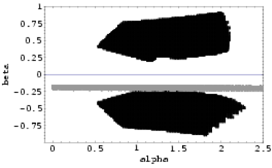
Figure 3: The black region is the experimentally allowed region predicted from a neutrino mass matrix with two zeros of eq. (2.7). The gray region is predicted from the up-quark masses at the GUT scale for the type $S_{2}$ in the case II with $h=1.3$.

Figure 5: The black region is the experimentally allowed region predicted from a neutrino mass matrix with two zeros of eq. (2.7). The gray region is predicted from the up-quark masses at the GUT scale for the type $F_{3}$ in the case III with $h=1.3$.

Figure 6: The black region is the experimentally allowed region predicted from a neutrino mass matrix with two zeros of eq. (2.7). The gray region is predicted from the up-quark masses at the GUT scale for the type $F_{4}$ in the case III with $h=1.3$.

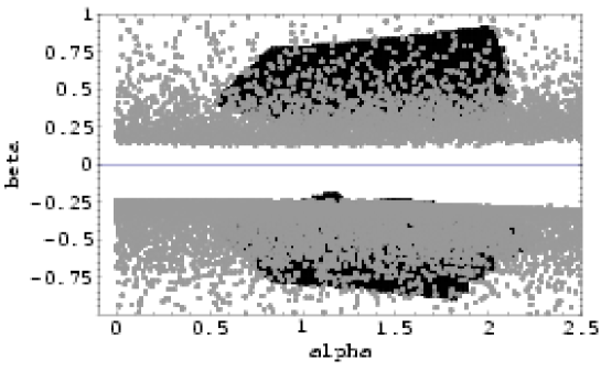
Figure 8: The black region is the experimentally allowed region predicted from a neutrino mass matrix with two zeros of eq. (2.7). The gray region is predicted from the up-quark masses at the GUT scale for the type $S_{2}$ in the case IV with $h=1.3$.

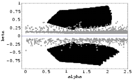
Figure 9: The black region is the experimentally allowed region predicted from a neutrino mass matrix with two zeros of eq. (2.7). The gray region is predicted from the up-quark masses at the GUT scale for the type $A_{1}$ in the case IV with $h=1.3$.

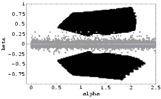
Figure 10: The black region is the experimentally allowed region predicted from a neutrino mass matrix with two zeros of eq. (2.7). The gray region is predicted from the up-quark masses at the GUT scale for the type $B_{1}$ in the case IV with $h=1.3$.

Figure 11: The black region is the experimentally allowed region predicted from a neutrino mass matrix with two zeros of eq. (2.7). The gray region is predicted from the up-quark masses at the GUT scale for the type $C_{1}$ in the case IV with $h=1.3$.

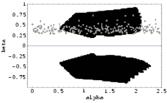
Figure 12: The black region is the experimentally allowed region predicted from a neutrino mass matrix with two zeros of eq. (2.7). The gray region is predicted from the up-quark masses at the GUT scale for the type $F_{3}$ in the case IV with $h=1.3$.

Figure 13: The black region is the experimentally allowed region predicted from a neutrino mass matrix with two zeros of eq. (2.7). The gray region is predicted from the up-quark masses at the GUT scale for the type $F_{4}$ in the case IV with $h=1.3$.

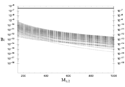
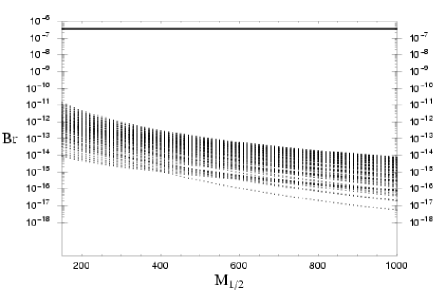
Figure 15: The predicted branching ratio of $\tau\rightarrow e\gamma$ process as a function of $M_{1/2}$ (GeV) taking $a_{0}=0$, $m_{0}=100\sim 1000\,{\rm GeV}$ for $\tan\beta=5\sim 50$ are shown. The left and right figure correspond to the type $S_{1}$ and $S_{2}$, respectively. The horizontal line is experimental upper bound.

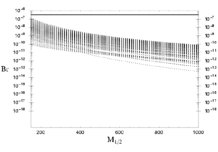
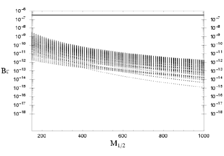
Figure 16: The predicted branching ratio of $\tau\rightarrow\mu\gamma$ process as a function of $M_{1/2}$ (GeV) taking $a_{0}=0$, $m_{0}=100\sim 1000\,{\rm GeV}$ for $\tan\beta=5\sim 50$ are shown. The left and right figure correspond to the type $S_{1}$ and $S_{2}$, respectively. The horizontal line is experimental upper bound.

Figure 17: The predicted baryon asymmetry of the universe are shown as a function of the degeneracy $\Delta M$. The region between horizontal lines is the observed value of baryon asymmetry $\eta_{B}$ [41]. The prediction is consistent with the observed value in the region of $\Delta M\simeq 10^{-3}$.

References

-
[1]
G. L. Fogli, E. Lisi, M. Marrone, D. Montanino, A. Palazzo and A.M. Rotunno,
Phys. Rev. D67 (2003), 073002;
J. N. Bahcall, M. C. Gonzalez-Garcia and C. Pea-Garay, JHEP 0302 (2003), 009;
M. Maltoni, T. Schwetz and J.W.F. Valle, Phys. Rev. D67 (2003), 093003;
P.C. Holanda and A. Yu. Smirnov, JCAP 0302 (2003), 001;
V. Barger and D. Marfatia, Phys. Lett. B555 (2003), 144;
M. Maltoni, T. Schwetz, M. Tórtola and J.W.F. Valle, hep-ph/0309130. -
[2]
Super-Kamiokande Collaboration, Y. Fukuda et al., Phys. Rev. Lett. 81 (1998), 1562;
ibid. 82 (1999), 2644; ibid. 82 (1999), 5194;
K. Nishikawa, Invited talk at XXI Lepton Photon Symposium, August 10-16,2003, Batavia, USA. - [3] Super-Kamiokande Collaboration, S. Fukuda et al., Phys. Rev. Lett. 86 (2001), 5651; ibid. 86 (2001), 5656.
- [4] SNO Collaboration, Q. R. Ahmad et al., Phys. Rev. Lett. 87 (2001), 071301; ibid. 89 (2002), 011301; ibid. 89 (2002), 011302; nucl-ex/309004.
- [5] KamLAND Collaboration, K. Eguchi et al., Phys. Rev. Lett. 90 (2003), 021802.
- [6] CHOOZ Collaboration, M. Apollonio et al., Phys. Lett. B466 (1999), 415.
- [7] H. Georgi and C. Jarlskog, Phys. Lett. B86 (1979), 297.
- [8] H. Fritzsch and Z-Z. Xing, Prog. Part. Nucl. Phys. 45 (2000), 1; and references therein.
-
[9]
P. S. Gill and M. Gupta, Phys. Rev. D57 (1998), 3971;
M. Randhawa, V. Bhatnagar, P. S. Gill and M. Gupta, Phys. Rev. D60 (1999), 051301;
S.K. Kang and C.S. Kim, Phys. Rev. D63 (2001), 113010;
M. Randhawa, G. Ahuja and M. Gupta, Phys. Rev. D65 (2002), 093016. - [10] P.H. Frampton, S.L. Glashow and D. Marfatia, Phys. Lett. B536 (2002), 79; Z. Xing, Phys. Lett. B530 (2002), 159; A. Kageyama, S. Kaneko, N. Shimoyama and M. Tanimoto, Phys. Lett. B538 (2002), 96; M. Honda, S. Kaneko and M. Tanimoto, JHEP 0309 (2003), 028; R. Barbieri, T. Hambye and A. Romanino, hep-ph/0302118.
- [11] J. Harvey, P. Ramond and D. Reiss, Phys. Lett. B92 (1980), 309; Nucl. Phys. B199 (1982), 223.
- [12] S. Dimopoulos, L. J. Hall and S. Raby, Phys. Rev. Lett. 68 (1992), 1984; Phys. Rev. D45 (1992), 4195.
- [13] P. Ramond, R. G. Roberts and G. G. Ross, Nucl. Phys. B406 (1993), 19.
- [14] Y. Achiman and T. Greiner, Nucl. Phys. B443 (1995), 3.
- [15] K. Hagiwara and N. Okamura, Nucl. Phys. B548 (1999), 60.
- [16] M. C. Chen and K. T. Mahanthappa, Phys. Rev. D62 (2000), 113007; ibid. 65 (2002), 053010; hep-ph/0212375.
-
[17]
D. Du and Z. Z. Xing, Phys. Rev. D48 (1993), 2349;
H. Fritzsch and Z. Z. Xing, Phys. Lett. B353 (1995), 114;
K. Kang and S. K. Kang, Phys. Rev. D56 (1997), 1511;
J. L. Chkareuli and C. D. Froggatt, Phys. Lett. B450 (1999), 158. -
[18]
H. Nishiura, K. Matsuda and T. Fukuyama, Phys. Rev. D60 (1999), 013006;
K. Matsuda, T. Fukuyama and H. Nishiura, Phys. Rev. D61 (2000), 053001. - [19] M. Bando and M. Obara, Prog. Theor. Phys. 109 (2003), 995.
- [20] M. Bando, S. Kaneko, M. Obara and M. Tanimoto, Phys. Lett. B580 (2004), 229.
- [21] Z. Maki, M. Nakagawa and S. Sakata, Prog. Theor. Phys. 28 (1962), 870.
- [22] See the Nishiura, Matsuda and Fukuyama in reference [18] for the matrix form of .
-
[23]
N. Haba, Y. Matsui, N. Okamura and M. Sugiura, Eur. Phys. J. C10 (1999) 677;
Prog. Theor. Phys. 103 (2000), 145;
N. Haba and N. Okamura, Eur. Phys. J. C14 (2000) 347;
N. Haba, N. Okamura and M. Sugiura, Prog. Theor. Phys. 103 (2000), 367. - [24] F. Borzumati and A. Masiero, Phys. Rev. Lett. 57 (1986), 961.
-
[25]
J. Hisano, T. Moroi, K. Tobe, M. Yamaguchi
and T. Yanagida, Phys. Lett. B357 (1995), 579;
J. Hisano, T. Moroi, K. Tobe and M. Yamaguchi, Phys. Rev. D53 (1996), 2442. -
[26]
J. Hisano, D. Nomura and T. Yanagida, Phys. Lett. B437 (1998), 351;
J. Hisano and D. Nomura, Phys. Rev. D59 (1999), 116005;
M.E. Gomez, G.K. Leontaris, S. Lola and J. D. Vergados, Phys. Rev. D59 (1999), 116009;
W. Buchmüller, D. Delepine and F. Vissani, Phys. Lett. B459 (1999), 171;
W. Buchmüller, D. Delepine and L.T. Handoko, Nucl. Phys. B576 (2000), 445;
J. Ellis, M.E. Gomez, G.K. Leontaris, S. Lola and D.V. Nanopoulos, Eur. Phys. J. C14 (2000), 319;
J. L. Feng, Y. Nir and Y. Shadmi, Phys. Rev. D61 (2000), 113005;
S. Baek, T. Goto, Y. Okada and K. Okumura, Phys. Rev. D63 (2001), 051701. -
[27]
J. Sato, K. Tobe, and T. Yanagida,
Phys. Lett. B498 (2001), 189;
J. Sato and K. Tobe, Phys. Rev. D63 (2001), 116010;
S. Lavignac, I. Masina and C. A. Savoy, Phys. Lett. B520 (2001), 269;
J. A. Casas and A. Ibarra, Nucl. Phys. B618 (2001), 171;
A. Kageyama, S. Kaneko, N. Simoyama and M. Tanimoto, Phys. Lett. B527 (2002), 206; Phys. Rev. D65 (2002), 096010. - [28] J. A. Casas and A. Ibarra, Nucl. Phys. B618 (2001), 171.
- [29] A. Kageyama, S. Kaneko, N. Simoyama and M. Tanimoto, Phys. Lett. B527 (2002), 206; Phys. Rev. D65 (2002), 096010.
- [30] J. Ellis, J. Hisano, M. Raidal and Y. Shimizu, Phys. Rev. D66 (2002), 115013.
- [31] MEGA Collaboration, M. L. Brooks et al., Phys. Rev. Lett. 83 (1999), 1521.
- [32] K. Inami, for the Belle collaboration, Talk presented at the 19th International Workshop on Weak Interactions and Neutrinos (WIN-03), October 6th to 11th, 2003, Lake Geneva, Wisconsin, USA.
- [33] K. Abe et al. (Belle collaboration), hep-ex/0310029.
- [34] S.T. Petcov, S. Profumo, Y. Takanishi and C.E. Yaguna, Nucl. Phys. B676 (2004), 453.
- [35] K. Inami, T. Hokuue and T. Ohshima, eConf C0209101 (2002) TU11 [hep-ex/0210036].
- [36] M. Fukugita and T. Yanagida. Phys. Lett. B175 (1986), 45.
-
[37]
M. Flanz, E. A. Paschos and U. Sarkar, Phys. Lett. B345 (1995), 248;
L. Covi, E. Roulet and F. Vissani, Phys. Lett. B384 (1996), 169;
A. Pilaftsis, Phys. Rev. D56 (1997), 5431. -
[38]
W. Buchmüller and M. Plümacher,
Phys. Lett. B389 (1996), 73; ibid. B431 (1998), 354;
Int. J. Mod. Phys. A15 (2000), 5047. -
[39]
M. Luty, Phys. Rev. D45 (1992), 455;
M. Plümacher, Z. Phys. C74 (1997), 549;
E. W. Kolb and M. S. Turner, The early universe, Redwood City, USA: Addison-Wesley (1990), (Frontiers in physics, 69);
M. Flanz and E. A. Paschos, Phys. Rev. D58 (1998), 113009;
- [40] H.B. Nielsen and Y. Takanishi, Phys. Lett. 507 (2001), 241.
- [41] D.N. Spergel et al., Astrophys. J. Suppl. 148 (2003), 175.
- [42] W. Buchmuller, P. Di Bari and M. Plumacher, Nucl. Phys. B643 (2002), 367; Phys. Lett. B547 (2002), 128.
- [43] G.F. Giudice, A. Notari, M. Raidal, A. Riotto and A. Strumia, Nucl. Phys. B685 (2004), 89.
- [44] A. Pilaftsis, Phys. Rev. D56 (1997), 5431; Int. J. Mod. Phys. A 14 (1999), 1811.
- [45] A. Pilaftsis and Thomas E.J. Underwood, hep-ph/0309342.
- [46] J. Ellis, M. Raidal and T. Yanagida, Phys.Lett. B546 (2002), 228.
- [47] G. C. Branco, R. Gonzalez Felipe, F. R. Joaquim, I. Masina, M. N. Rebelo and C. A. Savoy, Phys. Rev. D67 (2003), 073025.
- [48] E. K. Akhmedov, M. Frigerio and A. Yu. Smirnov, JHEP 0309 (2003), 021.
- [49] R. Gonzalez Felipe, F. R. Joaquim and B. M. Nobre, hep-ph/0311029.
- [50] C. H. Albright and S.M. Barr, hep-ph/0404095.
- [51] T. Hambye, Nucl. Phys. B633 (2002), 171.
- [52] T. Hambye, J. March-Russell and S. M. West, hep-ph/0403183.
-
[53]
M. Y. Khlopov and A. D. Linde,
Phys. Lett. B138 (1984), 265;
J. Ellis, J. E. Kim and D. V. Nanopoulos, Phys. Lett. B145 (1984), 181;
M. Kawasaki and T. Moroi, Prog. Theor. Phys. 93 (1995), 879.
M. Kawasaki, K. Kohri and T. Moroi, Phys. Rev. D 63 (2001), 103502; astro-ph/0402490.