Planck-Scale Effects on Global Symmetries:
Cosmology of Pseudo-Goldstone Bosons

Abstract

We consider a model with a small explicit breaking of a global symmetry, as suggested by gravitational arguments. Our model has one scalar field transforming under a non-anomalous $U(1)$ symmetry, and coupled to matter and to gauge bosons. The spontaneous breaking of the explicitly broken symmetry gives rise to a massive pseudo-Goldstone boson. We analyze thermal and non-thermal production of this particle in the early universe, and perform a systematic study of astrophysical and cosmological constraints on its properties. We find that for very suppressed explicit breaking the pseudo-Goldstone boson is a cold dark matter candidate.

I Introduction

It is generally believed that there is new physics beyond the standard model of particle physics. At higher energies, new structures should become observable. Among them, there will probably be new global symmetries that are not manifest at low energies. It is usually assumed that symmetries would be restored at the high temperatures and densities of the early universe.

However, the restoration of global symmetries might be not completely exact, since Planck-scale physics is believed to break them explicitly. This feature comes from the fact that black holes do not have defined global charges and, consequently, in a scattering process with black holes, global charges of the symmetry would not be conserved banks . Wormholes provide explicit mechanisms of such non-conservation Giddings_etal .

In the present article, we are concerned with the case that the high temperature phase is only approximately symmetric. The breaking will be explicit, albeit small. In the process of spontaneous symmetry breaking (SSB), pseudo-Goldstone bosons (PGBs) with a small mass appear. We explore the cosmological consequences of such particle species, in a simple model that exhibits the main physical features we would like to study.

The model has a (complex) scalar field $\Psi(x)$ transforming under a global, non-anomalous, $U(1)$ symmetry. We do not need to specify which quantum number generates the symmetry; it might be B-L, or a family $U(1)$ symmetry, etc. We assume that the potential energy for $\Psi$ has a symmetric term and a symmetry-breaking term

$$V=V_{sym}+V_{non-sym}$$ (1)

The symmetric part of the potential is

$$V_{sym}=\frac{1}{4}\lambda[|\Psi|^{2}-v^{2}]^{2}$$ (2)

where $\lambda$ is a coupling and $v$ is the energy scale of the SSB. This part of the potential, as well as the kinetic term $|\partial^{\mu}\Psi|^{2}$, are invariant under the $U(1)$ global transformation $\Psi\rightarrow e^{i\alpha}\Psi$.

Without any clue about the precise mechanism that generates $V_{non-sym}$, we work in an effective theory framework, where operators of order higher than four break explicitly the global symmetry. The operators would be generated at the Planck scale $M_{P}=1.2\times 10^{19}$ GeV and are to be used at energies below $M_{P}$. They are multiplied by inverse powers of $M_{P}$, so that when $M_{P}\rightarrow\infty$ the new effects vanish.

The $U(1)$ global symmetry is preserved by $\Psi^{\star}\Psi=|\Psi|^{2}$ but is violated by a single factor $\Psi$. So, the simplest new operator will contain a factor $\Psi$

$$V_{non-sym}=-g\frac{1}{M_{P}^{n-3}}|\Psi|^{n}\left(\Psi e^{-i\delta}+\Psi^{\star}e^{i\delta}\right)$$ (3)

with an integer $n\geq 4$. The coupling in (3) is in principle complex, so that we write it as $g\,e^{-i\delta}$ with $g$ real. We will consider that $V_{non-sym}$ is small enough so that it may be considered as a perturbation of $V_{sym}$. Even if (3) is already suppressed by powers of the small factor $v/M_{P}$, we will assume $g$ small. In fact, after our phenomenological study we will see that $g$ must be tiny.

To study the modifications that the small explicit symmetry breaking term induces in the SSB process, we use

$$\Psi=(\rho+v)e^{i\theta/v}$$ (4)

with new real fields $\rho(x)$ and the PGB $\theta(x)$. Introducing (4) in (3) we get

$$V_{non-sym}=-2\,g\,v^{4}\left(\frac{v}{M_{P}}\right)^{n-3}\cos{\left(\frac{\theta}{v}-\delta\right)}+\cdots$$ (5)

The dots refer to terms where $\rho(x)$ is present. We see from (5) that there is a unique vacuum state, with $<\theta>=\delta\,v$. To simplify, we redefine $\theta^{\prime}=\theta-\delta\,v$, and drop the prime, so that the minimum is now at $<\theta>=0$. From (5) we easily obtain the $\theta$ particle mass

$$m_{\theta}^{2}=2g\left(\frac{v}{M_{P}}\right)^{n-1}M_{P}^{2}$$ (6)

Although for the sake of generality we keep the $n$-dependence in (6), when discussing numerics and in the figures we particularize to the simplest case $n=4$, with the operator in (3) of dimension five. We will discuss in Section V what happens for $n>4$.

To fully specify our model, we finally write the couplings of the PGB $\theta$ to other particles. We have the usual derivative couplings to fermions gelmini ,

$${\cal L}_{\theta f\bar{f}}=\frac{g^{\prime}}{2\,v}\,(\partial_{\mu}\theta)\,\bar{f}\gamma^{\mu}\gamma_{5}f=g_{\theta f\bar{f}}\,\theta\,\bar{f}\gamma_{5}f$$ (7)

We have no reason to make $g^{\prime}$ very different from ${\cal O}(1)$. To have less parameters we set $g^{\prime}=1$ for all fermions and discuss in a final section about this assumption. Then

$$g_{\theta f\bar{f}}=\frac{m_{f}}{v}$$ (8)

The PGB $\theta$ couples to two photons through a loop,

$${\cal L}_{\theta\gamma\gamma}=\frac{1}{8}\,g_{\theta\gamma\gamma}\,\epsilon^{\mu\nu\rho\tau}F_{\mu\nu}F_{\rho\tau}\,\theta$$ (9)

where the effective coupling is $g_{\theta\gamma\gamma}=\frac{8\alpha}{\pi v}$. In the same way, there is a coupling to two gluons, ${\cal L}_{\theta gg}=\frac{1}{8}\,g_{\theta gg}\,\epsilon^{\mu\nu\rho\tau}G^{a}_{\mu\nu}G^{a}_{\rho\tau}\,\theta$ with $g_{\theta gg}=\frac{3\alpha_{s}}{\pi v}$. Couplings of $\theta$ to the weak gauge bosons do not play a relevant role in our study.

We have now the model defined. It has two free parameters: $g$, which is the strength of the explicit symmetry breaking term in (3), and $v$, which is the energy scale of the SSB appearing in (2).

At this point we would like to comment on the similarities and differences between our $\theta$-particle and the axion Weinberg:1977ma . There are similitudes because of their alike origin. For example the form of the coupling (7) to matter and (9) to photons is entirely analogous. A consequence is that we can borrow the supernova constraints on axions Raffelt_book to constrain our PGB. Another analogy is that axions are produced in the early universe by the misalignment mechanism three_papers and by string decay vilenkin and $\theta$-particles can also arise in both ways.

However, the fact that the $\theta$-particle gets its mass just after the SSB while axions become massive at the QCD scale introduces important differences. While in the axion case clearly only the angular oscillations matter and always one ends up with axion creation, in our model we need to work in detail the coupled evolution equations of the radial and angular part. We will need to establish when there are and when there are not angular oscillations leading to PGB creation.

Also, from the phenomenological point of view, the axion model is a one-parameter model while our model has two parameters $v$ and $g$. As we will see, this extra freedom makes the supernova constraints to allow a relatively massive $\theta$-particle, and we will need to investigate the consequences of the decay in the early universe. There is no analogous study for axions, simply because the invisible axion is stable, in practical terms.

Let us also mention other previous work on PGBs. In Mohapatra , the authors consider the SSB of B-L with explicit gravitational breaking so that they obtain a massive majoron. An important difference between their work and ours is that we consider non-thermal production, which is crucial for our conclusions about the PGB being a dark matter candidate. Also, there is previous work on explicit breaking of global symmetries Ross , and specifically on Planck-scale breaking Lusignoli . Cosmological consequences of some classes of PGBs are discussed in Hill . Finally, let us mention a recent paper Kazanas:2004kv where a massive majoron is considered in the context of a supersymmetric singlet majoron model ref3 . An objective of the authors of Kazanas:2004kv is to get hybrid inflation. Compared to our work, they consider other phenomenological consequences that the ones we study.

The article is organized as follows. We first discuss the particle properties of $\theta$. In Section III, we work out the cosmological evolution of the fields, focusing in thermal and non-thermal production, and discuss the relic density of PGBs. The astrophysical and cosmological bounds, and the consequences of the $\theta$ decay, are presented in Section IV. A final section discusses the conclusions of our work.

II $\theta$ - Mass And Lifetime

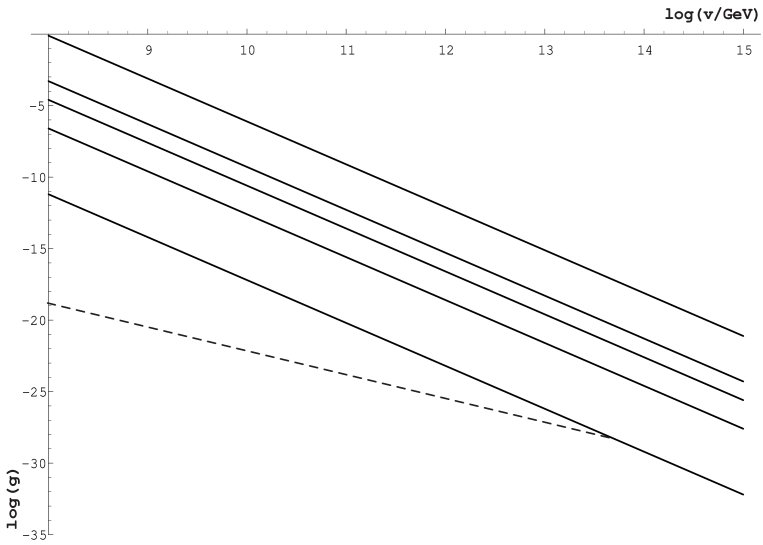
Figure 1: From bottom to the top, the five solid lines are the lines of constant mass, in the $g$,$v$ plane, for $m_{\theta}=2m_{e},\,2m_{\mu},\,2m_{p},\,2m_{b}$, and $2m_{t}$. The dashed line corresponds to the $\theta$ lifetime equal to the universe lifetime, $\tau=t_{0}$, when $\theta\rightarrow\gamma\gamma$ is the only available mode.

We have deduced the expression (6) that gives the mass of the $\theta$-particle as a function of $v$ and $g$. In terms of these two parameters, we plot in Fig.1 lines of constant mass, for masses corresponding to the thresholds of electron, muon, proton, bottom, and top final decay, $m_{\theta}=2m_{e},\,2m_{\mu},\,2m_{p},\,2m_{b}$, and $2m_{t}$.

The lifetime $\tau$ of the $\theta$-particle depends on its mass and on the effective couplings. A channel that is always open is $\theta\rightarrow\gamma\gamma$. The corresponding width is

$$\Gamma(\theta\rightarrow\gamma\gamma)=\frac{B_{\gamma\gamma}}{\tau}=g^{2}_{\theta\gamma\gamma}\;\frac{m^{3}_{\theta}}{64\pi}$$ (10)

where $B_{\gamma\gamma}$ is the branching ratio. When $m_{\theta}>2m_{f}$, the decay $\theta\rightarrow f\bar{f}$ is allowed and has a width

$$\Gamma(\theta\rightarrow f\bar{f})=\frac{B_{f\bar{f}}}{\tau}=g^{2}_{\theta f\bar{f}}\;\frac{m_{\theta}}{8\pi}\,\beta$$ (11)

where $\beta=\sqrt{1-4\,\left(\frac{m_{f}}{m_{\theta}}\right)^{2}}$.

For masses $m_{\theta}<2m_{e}$ the only available decay is into photons. When we move to higher $\theta$ masses, as soon as $m_{\theta}>2m_{e}$, we have the decay $\theta\rightarrow e^{+}e^{-}$. Actually, then the $\theta\rightarrow e^{+}e^{-}$ channel dominates the decay because $\theta\rightarrow\gamma\gamma$ goes through one loop. However, $\Gamma(\theta\rightarrow\gamma\gamma)\propto m_{\theta}^{3}$ whereas $\Gamma(\theta\rightarrow f\bar{f})\propto m_{\theta}$. By increasing $m_{\theta}$ we reach the value $m_{\theta}\simeq 150\,m_{e}$, where $\Gamma(\theta\rightarrow\gamma\gamma)\simeq\Gamma(\theta\rightarrow e^{+}\,e^{-})$. For higher $m_{\theta}$ the channel $\theta\rightarrow\gamma\gamma$ dominates again. If we continue increasing the $\theta$ mass and cross the threshold $2m_{\mu}$, the decay $\theta\rightarrow\mu^{+}\mu^{-}$ dominates over $\theta\rightarrow e^{+}e^{-}$ and $\theta\rightarrow\gamma\gamma$, because $g_{\theta f\bar{f}}$ is proportional to the fermion mass $m_{f}$. This would be true until $m_{\theta}\simeq 150\,m_{\mu}$, but before, the channel $\theta\rightarrow p\bar{p}$ opens, and so on. For larger masses, each time a threshold $2m_{f}$ opens up, $\theta\rightarrow f\bar{f}$ happens to be the dominant decay mode.

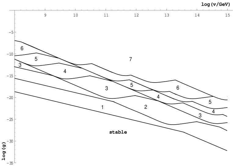
Figure 2: Zones corresponding to some ranges for the $\theta$ lifetime, $\tau$. At the bottom, we have the region of the parameter space leading to a stable $\theta$ ($\tau>t_{0}$), and at the top, the zone 7, where $\tau<1$ s. The other regions correspond to : $(1)\,t_{0}>\tau>10^{13}\,\rm s$; $(2)\,10^{13}\,\rm s>\tau>10^{9}\,\rm s$; $(3)\,10^{9}\,\rm s>\tau>10^{6}\,\rm s$; $(4)\,10^{6}\,\rm s>\tau>10^{4}\,\rm s$; $(5)\,10^{4}\,\rm s>\tau>300\,\rm s$ and $(6)\,300\,\rm s>\tau>1\,\rm s$.

Now we can identify in Fig.2 the regions with different lifetimes. We start with the stability region $\tau>t_{0}\simeq 4\times 10^{17}$ s wmap , the universe lifetime, a crucial region for the dark matter issue. When $m_{\theta}<2m_{e}$, $\tau=t_{0}$ along the dashed line in Fig.1 until $v\simeq 4\times 10^{13}$ GeV and along the line $m_{\theta}=2m_{e}$ for higher $v$. Below these lines, relic $\theta$ particles would have survived until now; in practical terms, for values of $g$ and $v$ in that region, we consider $\theta$ as a stable particle. Above the lines, $\tau<t_{0}$ and the particle is unstable. For future use, we define the ranges: $(1)\,t_{0}>\tau>10^{13}\,\rm s$; $(2)\,10^{13}\,\rm s>\tau>10^{9}\,\rm s$; $(3)\,10^{9}\,\rm s>\tau>10^{6}\,\rm s$; $(4)\,10^{6}\,\rm s>\tau>10^{4}\,\rm s$; $(5)\,10^{4}\,\rm s>\tau>300\,\rm s$; and $(6)\,300\,\rm s>\tau>1\,\rm s$.

III Cosmological production and PGB density

$\theta$-particles can be produced in the early universe by different mechanisms. There are non-thermal ones, like production associated with the $\theta$ field oscillations, and production coming from the decay of cosmic strings produced in the SSB. Also, there could be thermal production. In this section we consider these production mechanisms and the PGB density resulting from them.

Let us begin with the $\theta$ field oscillation production. The expansion of the universe is characterized by the Hubble expansion rate $H$,

$$H=\frac{1}{2t}=\sqrt{\frac{4\pi^{3}}{45}}\,\sqrt{g_{\star}}\,\frac{T^{2}}{M_{P}}$$ (12)

These relations between $H$ and the time and temperature of the universe, $t$ and $T$, are valid in the radiation era. For the period of interest, we take the relativistic degrees of freedom $g_{\star}=106.75$ KolbTurner . In the evolution of the universe, phase transitions occur when a symmetry is broken. When the universe cools down from high temperatures there is a moment when the potential starts changing its shape, and will have displaced minima. This happens around a critical temperature $T_{cr}\sim v$ and a corresponding critical time $t_{cr}$.

In our model, the explicit symmetry breaking is very small and the evolution equations of $\rho$ and $\theta$ are approximately decoupled. The temporal development leading $\rho$ and $\theta$ to the minimum occurs in different time scales, since the gradient in the radial direction is much greater than that in the angular one. The evolution happens in a two-step process. First $\rho$ goes very quickly towards the value $<\rho>=0$, and oscillates around it with decreasing amplitude (particle decay and the expansion of the universe work as a friction). Shortly after, $\rho$ will be practically at its minimum. In this first step where $\rho$ evolves, $\theta$ does not practically change, maintaining its initial value $\theta_{0}$, which in general is not the minimum, i.e., $\theta_{0}\neq 0$. $\theta$ evolves towards the minimum once the first step is completely over. This is the second step where the field $\theta$ oscillates around $<\theta>=0$.

We have confirmed these claims with a complete numerical treatment of the full evolution equations, using the effective potential taking into account finite temperature effects. We summarize our results in Appendix A.

Hence, we can write the following $\rho$-independent evolution equation for $\theta$

$$\ddot{\theta}(t)+3H\,\dot{\theta}(t)+m_{\theta}^{2}\,\theta=0$$ (13)

Here overdot means $d/dt$. We do not introduce a decay term in the motion equation (13) and will treat the $\theta$ decay in the usual way. We can do it because $\theta$ has a lifetime $\tau$ that is much greater than the period of oscillations.

Oscillations of the $\theta$ field start at a temperature $T_{osc}$ such that $3H(T_{osc})\sim m_{\theta}$ and this will be much later than the period of $\rho$ evolution provided $T_{osc}\ll T_{cr}\sim v$. This is equivalent to

$$g^{1/2}\,\ll\,3\times 10^{-3}\,\left(\frac{10^{11}\,\rm GeV}{v}\right)^{-1/2}$$ (14)

We shall see that the phenomenologically viable and interesting values of $g$ are very tiny, so that we can assume that the inequality (14) is fulfilled.

Since the $\theta$ oscillations are decoupled from $\rho$ oscillations, $\theta$ production is equivalent to the misalignment production for the axion and we can use those results three_papers . The equation of motion (13) leads to coherent field oscillations that correspond to non-relativistic matter and the coherent field energy corresponds to a condensate of non-relativistic $\theta$ particles.

We define $\rho_{osc}$ and $n_{osc}$ as the energy density, and number density respectively, of the PGBs coming from the $\theta$ oscillations. The energy stored initially is

$$\rho_{osc}=m_{\theta}\,n_{osc}\simeq\frac{1}{2}\,m_{\theta}^{2}\theta_{0}^{2}$$ (15)

The initial angle is unknown, $\theta_{0}/v\in[0,2\pi)$, so that we expect it to be of order one, $\theta_{0}/v\sim 1$. In the following we will set $\theta_{0}=v$. Barring an unnatural $\theta_{0}$ fine tuned extremely close to 0, other choices of $\theta_{0}$ would lead essentially to the same conclusions we reach.

Let us now consider production of PGBs by cosmic string decays. When our $U(1)$ symmetry is spontaneously broken, a network of (global) strings is formed vilenkin . These strings evolve in the expanding universe and finally decay into PGBs, at a time $t_{str}$ given by $m_{\theta}t_{str}\sim 1$, which is of the order of $t_{osc}$. The same issue has been extensively studied for the axions and we can borrow the results Davis ; Harari . Unfortunately, there are different calculations that do not agree among them. To be conservative, we take the least restrictive result, namely, the one giving less particle production. That is Harari

$$n_{str}(t_{str})\approx\frac{v^{2}}{t_{str}}$$ (16)

This is of the same order of magnitude as the PGB density at time $t_{str}$ due to $\theta$-oscillation production.

Thus, the total number density of non-thermally produced PGBs is

$$n_{non-th}=n_{osc}+n_{str}$$ (17)

Let us now consider the thermal production of PGBs. Any species that couples to the particles present in the early universe and has a production rate $\Gamma$ larger than the Hubble expansion rate $H$ during a certain period will be thermally produced. Whether such a period exists or not has been investigated for the axion Turner:1986tb ; MRZ . We adapt the axion results, taking into account the different magnitude of the gluon-gluon vertex, and conclude that for

$$v<7.2\times 10^{12}\,{\rm GeV}\equiv v_{th}$$ (18)

there is always thermal production of $\theta$ in the early universe. However, for larger values of $v$, $\theta$ interacts so weakly that $\Gamma<H$ always, or $\Gamma>H$ only for such a brief period of time that in practice there is no thermal production. We denote this region by (I) in Fig.3.

When $v<v_{th}$, the $\theta$ species actually interacts with the plasma in the following range of temperature $T$

$$v\geq T\geq\frac{v^{2}}{1.8\times 10^{14}\rm GeV}\equiv T_{end}$$ (19)

and a thermal population of $\theta$ is created with a number density

$$n_{th}=\frac{\zeta(3)}{\pi^{2}}\,T^{3}\simeq 0.12\,T^{3}$$ (20)

We should now reconsider the fate of the non-thermal PGBs in (17), since a thermalization period (19) may be at work. For this discussion we shall use the fact that $\theta$-oscillations and string decay start at about the same temperature, $T_{osc}\sim T_{str}$. Let denote this common temperature where non-thermal production starts by $T_{\ast}$. When $v<v_{th}$, we have to distinguish between two possible cases. First, if $T_{\ast}<T_{end}$, non-thermal $\theta$ are born after the thermalization period is over. We end up having both a thermal $n_{th}$ and a non-thermal $n_{non-th}$ densities, and a total density given by the sum $n_{\theta}=n_{th}+n_{non-th}$. This first case corresponds to values of $v$ and $g$ indicated in Fig.3 by regions (II) and (III); in (II) $n_{non-th}>n_{th}$, while in (III) $n_{th}>n_{non-th}$. The second case corresponds to having $T_{\ast}>T_{end}$; if this is the case, non-thermal PGBs will be in contact with the thermal bath and will consequently thermalize. Indeed, independently of details, we end up the period corresponding to (19) with $n_{\theta}=n_{th}$ given in (20). The region (IV) in Fig.(3) is where such complete thermalization happens.

A word of caution is now in order. When $T_{\ast}>v$, radial and angular oscillations are not decoupled. The analysis is not as simple as we presented before: the oscillations cannot be approximated by harmonic ones, and depend on initial conditions. However, if $v<v_{th}$, the PGBs get thermalized in any case, so that we have not to worry about the non-thermal production details. For $v>v_{th}$ (and still $T_{\ast}>v$), since there is no thermalization, the final density is $n_{\theta}=n_{non-th}$. Admittedly, we have no general formula for the density in this case, represented by (V) in Fig.3. In this region, $\theta$ lifetimes are so small that the particle does not play any cosmological role at all.

Summarizing, a number density of $\theta$ particles always appears in the early universe. In regions (II), (III), and (IV), the thermal density is $n_{th}(T=T_{D})$ at decoupling temperature $T_{D}$ (the temperature where $\Gamma=H$). In regions (I), (II), and (III) there is also a non-thermal density $n_{non-th}$ at formation temperature $T=T_{\ast}$.

As usual, the expansion of the universe dilutes these densities. Eventually, if the particle is unstable it will decay. The issue of unstable $\theta$ and effects of the decay will be worked out in Section IV, and here we focus on stable $\theta$ particles, since certainly they would be dark matter. To calculate the relic density of $\theta$ today, apart from the expansion effect, one has to take into account the transferred entropy to the thermal bath, due to particle-antiparticle annihilations. We follow the standard procedure (see KolbTurner ), and find that the number density today is

$$n(T_{0})=\frac{g_{\star s}(T_{0})}{g_{\star s}(T_{1})}\left(\frac{T_{0}}{T_{1}}\right)^{3}n(T_{1})$$ (21)

where $T_{1}=T_{D}$ for $n_{th}$ and $T_{1}=T_{\ast}$ for $n_{non-th}$, and $T_{0}=2.7K$ is the photon temperature today. We take $g_{\star s}(T_{1})=106.75$ and $g_{\star s}(T_{0})=43/11$.

With all that, we can calculate the cosmological density of $\theta$ particles that we would have today, $n_{\theta}(t_{0})$, and the corresponding energy density normalized to the critical density $\rho_{c}$,

$$\Omega_{\theta}=\frac{m_{\theta}\,n_{\theta}(t_{0})}{\rho_{c}}$$ (22)

with $\rho_{c}=0.5\times 10^{-5}\,\rm GeV\,cm^{-3}$ PDG2002 .

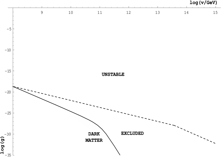
Figure 4: Properties of $\theta$ before considering the astrophysical constraints and the effects of the decay. Above the dashed line of the plot we have the region of $g,\,v$ where $\theta$ is unstable. The solid line corresponds to $\Omega_{\theta}=0.3$. The interesting dark matter region is labeled in the plot. The region between the solid and dashed lines is excluded because $\theta$ is stable and $\Omega_{\theta}>0.3$.

All cosmological data available lead to a dark matter contribution $\Omega_{DM}\simeq 0.3$ wmap . In Fig.4 we plot the line $\Omega_{\theta}=0.3$. We will see in Section IV that part of this line is excluded. Clearly, values of $g$ and $v$ along the non-excluded part of the line would imply the density needed to fit the cosmological observations. Our $\theta$ particle is a dark matter candidate provided $g$ and $v$ are on the line, or not far, in such a way that $\Omega_{\theta}$ is still a substantial fraction of 0.3. We stress that in the region of interest for dark matter it is the non-thermal production that dominates (see Fig.3). Thus, the produced PGBs are non-relativistic and would be cold dark matter. Values for $\Omega_{\theta}$ much smaller than $\sim 0.3$ are allowed but not cosmologically interesting. On the other side of the line, but still in the stability region, we have the excluded region $\Omega_{\theta}>0.3$.

IV Astrophysical and cosmological Constraints

PGBs would be emitted from the hot stellar cores since nucleons, electrons and photons initiate reactions where $\theta$ is produced. Provided $\theta$ escapes the star, the emission leads to a novel energy loss channel, which is constrained by stellar evolution observations using what is nowadays a standard argument Raffelt_book . The limits we find for $v$ are similar to the limits found for the Peccei-Quinn scale PDG2002 because the coupling of $\theta$ to matter is the same of the axion. We get the bound

$$v\gtrsim 3.3\times 10^{9}\,\rm GeV$$ (23)

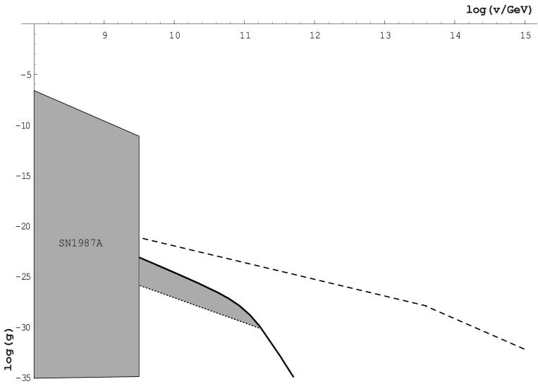
Figure 5: The astrophysical constraints forbid the shadow region labeled SN1987A. The other shadow region corresponds to stable particles ($\tau>t_{0}$), yet the contribution to the photon background is too high and thus this region is forbidden. To help the reader, we also plot the line $\Omega_{\theta}=0.3$ (solid) and the border between stable and unstable PGBs (dashed).

that is shown in Fig.5.

We see that the astrophysical constraint is on $v$, but not on $g$, so that we may have relatively massive PGBs, while in the axion case this leads to $m_{a}\lesssim O(10^{-3}{\rm eV})$, i.e., to forbid the existence of relatively massive axions. This makes the PGB in our model an unstable particle, at variance with the invisible axion.

Let us now investigate the region where $\theta$ is unstable, see Fig.4. The cosmological effects of the decay will depend on the lifetime $\tau$, mass $m_{\theta}$, and number density $n_{\theta}$ at the moment of the decay. These properties depend on the parameters $g$ and $v$. Observational data will help us to constrain different regions of the $g$, $v$ parameter space. We will use several pieces of data, depending on when the $\theta$ decay occurs. To do this systematically, it is convenient to distinguish between the following time ranges, plotted in Fig.2

$${\rm range\,1}: t_{0} \quad>\;t\;>\quad t_{\rm rec}\simeq 10^{13}\,\rm s$$

$${\rm range\,2}: t_{\rm rec} \quad>\;t\;>\quad t_{\rm c}\simeq 10^{9}\,\rm s$$

$${\rm range\,3}: t_{\rm c} \quad>\;t\;>\quad t_{\rm th}\simeq 10^{6}\,\rm s$$

$${\rm range\,4}: t_{\rm th} \quad>\;t\;>\quad t_{\rm He}\simeq 10^{4}\,\rm s$$

$${\rm range\,5}: t_{\rm He} \quad>\;t\;>\quad t_{\rm endBBN}\simeq 300\,\rm s$$

$${\rm range\,6}: t_{\rm endBBN} \quad>\;t\;>\quad t_{\rm BBN}\simeq 1\,\rm s$$

We do not consider times earlier than $t_{\rm BBN}$ since there are no observational data that give us any constraint at that times. The physical meaning of the chosen times are

• $t_{\rm rec}$ is the time of recombination, i.e., the moment at which photons last scattered with matter, when free electrons present in the cosmic plasma were bounded into atoms;

• $t_{\rm c}$ is the time at which the rate of Compton scattering $e\gamma\rightarrow e\gamma$ becomes too slow to keep kinetic equilibrium between photons and electrons;

• $t_{\rm th}$ is the time at which the double-Compton scattering $e\gamma\rightarrow e\gamma\gamma$ decouples;

• $t_{\rm He}$ is the time at which the energy of the Cosmic Background Radiation (CBR) is low enough to permit photons of energy $\sim 10$ MeV to photodissociate ⁴He nuclei;

• $t_{\rm endBBN}$ is the time at which the Big Bang Nucleosynthesis (BBN) finishes;

• $t_{\rm BBN}$ is the time at which BBN begins.

We can constrain the parameters $v$ and $g$ because the photon spectrum would be distorted by $\theta$ decay products, and the abundances of the light elements would be altered. We will discuss this in the next two subsections.

Effects on the photon spectrum

The products of the $\theta$ decay can be either photons or fermions. When the decay products are fermions it is important to note that if the number density of the created fermions is higher than the photon density of the CBR, these fermions immediately annihilate into photons, since we are considering decays produced after the $e^{+}e^{-}$ annihilation in the early universe. The distinction between the two channels will be important only when the $\theta$-decay occurs in the time ranges 1 and 2, since in the other regions photons and fermions thermalize.

When $\tau$ is in the range 1, it is convenient to distinguish between two regions (see Figs.1 and 2). In the region where $m_{\theta}<2\,m_{e}$, $\theta$ decays only into photons. The products of the other region are mainly $e^{-}$ and $e^{+}$, but the values of $v$ and $g$ in this region are such that the number density of the created fermions is higher than the CBR photon density. Then, in all the time range 1, the final products are photons, but for $m_{\theta}>2\,m_{e}$ we use $\tau$ for the $\theta\rightarrow e^{+}e^{-}$ decay. Photons produced in this range stream freely and contribute to the diffuse photon background of the universe. One can compute the present energy flux of photons per energy and solid angle interval coming from $\theta$-decay masso&toldra

$$\frac{d^{2}\mathcal{F}_{E}}{dEd\Omega}=\frac{1}{2\pi}\,\frac{n_{\theta}(t_{0})}{\tau\,H_{0}}\left(\frac{E}{m_{\theta}/2}\right)^{3/2}\exp{\left[-\frac{2}{3}\,\frac{1}{\tau\,H_{0}}\left(\frac{E}{m_{\theta}/2}\right)^{3/2}\right]}$$ (24)

where $H_{0}$ is the Hubble constant today and $n_{\theta}(t_{0})$ is the number density of $\theta$ that we would have today if it had not decayed. The predicted flux (24) is bounded by the observational limits Ressell&Turner on the photon background flux in the energy range of interest. This restriction excludes all the region in the $v$, $g$ parameter space corresponding to time range 1. Taking into account that even for $\tau>t_{0}$ a small fraction of PGBs have decayed into photons, we can also prohibit part of the parameter space that corresponds to stable particles with $\Omega\lesssim 0.3$ (see Section III). In Fig. 5 we plot this excluded region.

In range 2, Compton scattering is not effective in maintaining kinetic equilibrium between the $e^{-}$ and the $\gamma$ of the CBR. Depending on the precise values of $g$ and $v$, $\theta\rightarrow e^{+}e^{-}$, $\theta\rightarrow\mu^{+}\mu^{-}$ or $\theta\rightarrow\gamma\gamma$ will be the dominant decay. The induced charged leptons, carrying large energy, outnumber the existing CBR electrons. Different processes now compete; one is scattering of these hot electrons and muons with CBR photons. Another is $e^{+}e^{-}$ and $\mu^{+}\mu^{-}$ annihilations that give high energy photons, which heat CBR electrons. The last is high energy photons produced in the decay $\theta\rightarrow\gamma\gamma$, that also scatter and heat CBR electrons which in turn scatter with CBR photons. Whatever process is more important (it depends on the $g$, $v$ values), the result is a distortion of the photon spectrum, parameterized by the Sunyaev-Zeldovich parameter $y$ S-Z . The energy $\Delta E$ dumped to the CBR, relative to the energy of the CBR itself is constrained by data on CBR spectrum PDG2002

$$\frac{\Delta E}{E_{CBR}}\simeq 4y\lesssim 4.8\times 10^{-5}$$ (25)

where $\Delta E=m_{\theta}\,n_{\theta}$. The experimental bound (25) rules out all the $g$ and $v$ values that would imply a lifetime $\tau$ in the time range 2.

In the range 3, Compton scattering is fast enough to thermalize the products of the $\theta$-decay occurring in this range. This is because even in the region where the products are neither photons nor $e^{+}\,e^{-}$, the final particles will be photons in any case. In this region the $e\gamma\rightarrow e\gamma\gamma$ processes are not effective so the photon number cannot be changed. So, after thermalization, one obtains a Bose-Einstein CBR spectrum with a chemical potential, $f=\left[\exp{(E+\mu)/T}-1\right]^{-1}$, instead of a black-body spectrum. The relation between $\mu$ and $\Delta E$ is Toldra

$$\left(\frac{4}{3}\,\frac{\zeta(2)}{\zeta(3)}-\frac{\zeta(3)}{\zeta(4)}\right)\,\mu=\frac{\Delta E}{E_{CBR}}-\frac{4}{3}\,\frac{\Delta n_{\gamma}}{n_{\gamma}}$$ (26)

($\zeta(n)$ is Riemann’s zeta function). The parameter $\mu$ is very well constrained by CBR data PDG2002 that gives $|\mu|<9\times 10^{-5}$. This value rules out all the $g$, $v$ region that would give $\tau$ in the time range 3.

For times before the range 3, both Compton and double Compton scattering are effective, so the decay products thermalize with the CBR, without disturbing the black body distribution but changing the evolution of the temperature of the thermal bath. This temperature variation leads to a change in the photon number, and thus to a decrease on the parameter $\eta\equiv n_{b}/n_{\gamma}$. The knowledge we have on the value of this parameter at $t_{\rm rec}$ wmap and $t_{\rm endBBN}$ Sarkar allows to constrain the $g$, $v$ region that would give lifetimes $\tau$ in the time ranges 4 and 5. Although the corresponding restriction is quite poor (it is essentially $\Delta E/E_{CBR}\lesssim 1$), yet it excludes the parameter space corresponding to the ranges 4 and 5. However, constraints from the effects of the $\theta$-decay on the light element abundances are much more restrictive in these ranges, as we will examine in the next subsection.

Effects on the abundances of the light elements

The period of primordial nucleosynthesis is the earliest epoch where we have observational information. Also, the theoretical predictions of the primordial yields of light elements are robust. The agreement with observation is considered one of the pillars of modern cosmology. The $\theta$ decays, and the $\theta$ particle itself, might modify the abundances of the light elements, which implies restrictions on the $v$, $g$ parameters.

First, we consider how the decays of a PGB affect the abundances of the light elements after they are synthesized, i.e., after $t_{\rm endBBN}$. One of the consequences of the decay is the production of electromagnetic showers in the radiation-dominated plasma, initiated by the decay products. As a result, photons of energy $\sim$10 MeV scatter and photodissociate light elements. This scattering occurs after $t_{\rm He}$, because before $t_{\rm He}$, the collision of these photons with the CBR is more probable than with the light elements. In time range 4, the photodissociated element is deuterium (if $m_{\theta}>10$ MeV) Sarkar while in time ranges 3 and 2 there is helium photodissociation (if $m_{\theta}>100$ MeV), with the subsequent production of deuterium. Observational data for the abundance of deuterium constraint all these processes. When $\theta$ decays into quarks which hadronize subsequently, hadronic showers can also be produced (if $m_{\theta}\sim 1$ GeV). These processes dissociate ⁴He before $t_{\rm He}$, overproducing deuterium and lithium. All these constraints, that are summarized in Sarkar , exclude all the $g$ and $v$ values that give $\tau$ in the time ranges 2,3,4 and 5, provided mass conditions are fulfilled for each case. However, values from ranges 2,3,4 and 5 that do not satisfy the proper mass restrictions, are anyway excluded by the constraints we considered in the former subsection.

The other effect on the light element abundances arises because the $\theta$ particle would modify the BBN predictions. The presence of $\theta$ and, more important, the presence of the relativistic products of the $\theta$-decay, accelerate the expansion rate of the universe in the relevant BBN period and modify the synthesis of the light elements. The decay of the $\theta$ boson is also a source of entropy production, which alters the temperature evolution of the universe. This changes the number of photons (and the value of $\eta$) and produces an earlier decoupling of neutrinos. Then the relation between $T_{\nu}$ and $T_{\gamma}$ is changed, with potential effects on the BBN physics. It is important to note that this production of entropy never rises the temperature of the universe Turner , and does not lead to several successive BBN periods. All these effects in BBN have been implemented Turner2 in the usual code, which allows to constrain the quantity $\Delta E/n_{\gamma}$. As a result, some of the values of $g$, $v$ that would give $\tau$ in the time range 6 are ruled out. The potential effects of hadronic showers, that we have mentioned earlier, also would modify the BBN results Sarkar , allowing us to exclude part of the range 6, but not all of it.

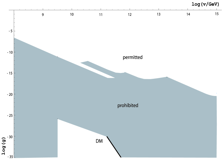
Figure 6: The prohibited region, using all constraints we have studied, is in shadow. In white, we show the allowed region. The solid line corresponds to $\Omega_{\theta}=0.3$.

All the results exposed in this section are summarized in Fig.6. There, we can see that after our systematic study, it turns out that all the zone of parameters that lead to lifetimes between about 1 s and $t_{0}$ is ruled out. Only a small zone corresponding to range 6 is allowed.

V Discussion and Conclusions

Gravitational arguments suggest that global symmetries are explicitly violated. We describe this violation using an effective theory framework that introduces operators of order higher than four, suppressed by inverse powers of the Planck mass. These operators are considered as a perturbation to the (globally) symmetric part of the potential.

The SSB of global symmetries with a small explicit breaking leads to PGBs: Goldstone bosons that have acquired a mass. Equivalent to the appearance of a mass for the boson, there is no longer an infinity of degenerate vacua.

In this article we have studied the cosmology of the PGB $\theta$ that arises in a model containing a scalar field with a potential that can be divided in a part that has a global non-anomalous $U(1)$ symmetry and another part with gravitationally induced terms that are $U(1)$ violating. In our analysis we let vary two parameters of the model: the SSB breaking scale, $v$, and the coupling $g$ of the Planck-induced term in the potential. We have analyzed the evolution of the field towards the vacuum in a phase transition in the early universe. It occurs in a two-step process: first the radial part attains its minimum in a relatively short time and second the angular part of the field starts oscillating well after the first step is over. The $\theta$ field oscillations correspond to non-relativistic matter. We have calculated the density of $\theta$ particles born through this mechanism and also through the decay of cosmic strings created at the SSB. There might also be thermal production of PGBs in the early universe and also there might be thermalization of PGBs produced non-thermally; these issues have been fully analyzed in our article.

A variety of arguments constrain the parameters $v$ and $g$ of $\theta$. There are astrophysical constraints coming from energy loss arguments. There are also cosmological bounds. When the particle is stable its density cannot be greater than about the critical density, otherwise the predicted lifetime of the universe would be too short. If the particle is unstable the decay products may have a cosmological impact. We have watched out for effects of the decay products on the CBR and on the cosmological density of light elements.

We have considered all the above potential effects and used empirical data to put constraints on $g$ and $v$. We have been led to exclude the region of the $g$, $v$ parameter space indicated in Fig.6.

In Fig.6. we see that there are two allowed regions in the plot. First, in the upper part of the plot there is an allowed region. It is where $\tau<$ 1 s, except the tooth at values that are about $v\sim 10^{11}$ GeV and $g\sim 10^{-13}$ that corresponds to 1 s $<\tau<$ 300 s (part of zone 6 in Fig.2). For a $\theta$ that has the parameters corresponding to this first region, it will definitely be extremely difficult to detect the particle. Also, in any case, it will have no cosmological relevance.

The second permitted zone of the figure is where $\theta$ is dark matter, at the bottom of the plot. It would be an interesting cold dark matter candidate provided the values of $g$ and $v$ are not far from the solid line in Fig.6. There is an upper limit to the mass $m_{\theta}$ in the allowed region where $\theta$ is a dark matter candidate

$$m_{\theta}\,\lesssim\,20\,\rm eV$$ (27)

A way to detect $\theta$ would be using the experiments that try to detect axions which make use of the two-photon coupling of the axion. Since a similar coupling to two photons exists for the PGB, we would see a signal in those experiments Masso:2002ip . The detection techniques use coherent conversion of the axion to photons, which implies that in order that $\theta$ would be detected, we should have $m_{\theta}<10^{-3}$ eV.

For $\theta$ be dark matter, we notice that the values of $g$ have to be very small

$$g<10^{-30}$$ (28)

We do not conclude that these values are unrealistically small. Without any knowledge of how gravity breaks global symmetries it would be premature to argue for or against the order of magnitude (28). For example, in 0009030 , Peccei elaborates about the explicit gravity-induced breaking of the Peccei-Quinn symmetry, and gives the idea that perhaps the finite size of a black hole when acting on microscopic processes further suppresses Planck-scale effects.

Apart from that, there is an easy way to get PGBs as dark matter candidates for values of $g$ not as tiny as in (28). Notice that to work out the most simple case, we have considered $n=4$ in Eq.(3). It suffices to consider more general potentials

$$V_{non-sym}=-\tilde{g}\frac{1}{M_{P}^{n+m-4}}|\Psi|^{n}\left(\Psi^{m}e^{-i\delta}\,+\,{\rm h.c.}\ \right)$$ (29)

with $n,m$ integers. In the present article we made $n=4$, $m=1$. If we take greater values, we get a suppression of the symmetry breaking term due to extra factors $v/M_{P}$ and we may allow values for $\tilde{g}$ higher than the ones obtained for $g$. In order of magnitude, for $v\sim 10^{11}$ GeV, we see that taking operators of dimension $n+m=8$ or $9$ we have a PGB that is a dark matter candidate, but now with $\tilde{g}\sim{\cal O}(1)$. In building the model we should have a reason for having the order of the operators starting at $n+m>5$. The standard way is to impose additional discrete symmetries in the theory.

Finally, we would like to comment on having put $g^{\prime}=1$ in (7). We could, of course, maintain $g^{\prime}$ free, even we could let $g^{\prime}$ be different for each fermion, but, in our opinion, the introduction of extra parameters would make the physical implications of our model much less clear. This is why we fixed $g^{\prime}=1$, but now it is time to think what happens for other values of $g^{\prime}$.

The coupling $g^{\prime}$ appears accompanying a factor proportional to the mass of the fermion and inversely proportional to the energy breaking scale $v$, as expected for real and pseudo Goldstone bosons. When a fermion has a $U(1)$ charge, we have no reason to expect that $g^{\prime}$ is much different than ${\cal O}(1)$, but if a fermion has vanishing $U(1)$ charge then the coupling of $\theta$ to this fermion may only go through loops, and consequently we have a smaller $g^{\prime}$. In this case, an important change concerns the astrophysical bound. Since $g_{\theta NN}$ is smaller than $m_{N}/v$, the bound from supernova is weakened and values of $v$ smaller than $3.3\times 10^{9}$ GeV would be allowed. Another effect is that the bounds coming from the cosmological effects of the $\theta$ decay are relaxed, since the lifetimes are longer when $g^{\prime}$ is smaller. However, this does not mean that part of the prohibited region in Fig.6 would be allowed. We have to take into account that non-thermal production is not altered when changing $g^{\prime}$ and therefore the bound $\Omega_{\theta}<$ 0.3 leads to strong restrictions in the $g,v$ parameter space. Also, $\theta$ thermal production is suppressed with smaller $g^{\prime}$.

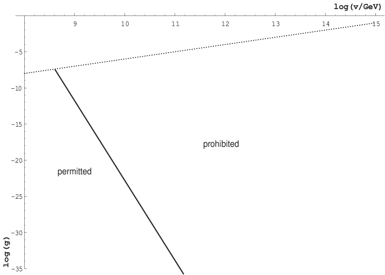
Figure 7: Permitted and prohibited regions in the limit $g^{\prime}\rightarrow 0$. The solid line is $\Omega_{\theta}=0.3$ and the dotted line is $T_{\ast}=v$. In the upper part of the dotted line we have no reliable way to calculate $\Omega_{\theta}$.

We would like to show graphically what would happen for very small $g^{\prime}$, and with this objective we show in Fig.7 the permitted and the prohibited regions in the limit $g^{\prime}\rightarrow 0$. At the view of the result, we conclude that one may have PGB as a dark matter candidate for much larger values of $g$ than obtained before in (28).

Appendix A

A.1 How to obtain the effective potential $V_{eff}$

We present here in some detail how to find the effective potential that gives us a complete description of the physics involved in our model. Following the standard procedure Quiros , taking into account the finite temperature effects, we are led to a new contribution to $V_{sym}$, which is given by

$$V^{\beta}=\frac{1}{2\pi^{2}\beta^{4}}J_{B}[m^{2}\beta^{2}]=\frac{1}{2\pi^{2}\beta^{4}}\int_{0}^{\infty}\,dx\,x^{2}\ln\left[1-e^{-\sqrt{x^{2}+\beta^{2}m^{2}}}\right]$$ (30)

where $J_{B}$ is the thermal bosonic function and $\beta=1/T$, and $m^{2}=-\frac{1}{2}\lambda v^{2}+\lambda\Psi^{\star}\Psi+\frac{1}{2}\lambda T^{2}$ is the effective mass. With (30), we see the behavior of the finite temperature effective potential. For practical applications, it is convenient to use a high temperature expansion of $V^{\beta}$ Dolan_Jackiw written in the form

$$V^{\beta}\simeq\frac{1}{24}m^{2}T^{2}-\frac{1}{12\pi}m^{3}T-\frac{1}{64\pi^{2}}m^{4}\ln\frac{m^{2}/T^{2}}{223.63}$$ (31)

where we have neglected terms independent of the field. The effective potential must contain the explicit symmetry-breaking term of our model, $V_{non-sym}$. Using for $\Psi$ the parametrization $\Psi=\phi\,e^{i\theta/v}$, the expression for this term is

$$V_{non-sym}=-2g\frac{\phi^{n+1}}{M_{P}^{n-3}}\cos\left(\frac{\theta}{v}\right)$$ (32)

Thus, our effective potential will be written as the sum of three terms

$$V_{eff}=V_{sym}+V^{\beta}+V_{non-sym}$$ (33)

A.2 How to find $T_{cr}$

SSB of $V_{eff}$ is triggered at a critical temperature $T_{cr}$ corresponding to time $t_{cr}$, and instead of having a minimum at $\phi=0$, a local maximum appears. $T_{cr}$ is the temperature when the second derivative of $V_{eff}$ at $\phi=0$ cancels. In calculating the derivative of $V_{eff}$, we find that

$$\frac{\partial V_{eff}}{\partial\phi}=\phi\cdot f(\phi,T)$$ (34)

$f(\phi,T)$ contains all the information we need to find both $T_{cr}$ and the minimum of the potential as a function of $T$ (writing $f(\phi,T)=0$ and solving for $\phi$). The second derivative of $V_{eff}$ at its origin is

$$\left.\frac{\partial^{2}V_{eff}}{\partial\phi^{2}}\right|_{\phi=0}=f(\phi,T)|_{\phi=0}+(\phi\,f^{\prime}(\phi,T))|_{\phi=0}=f(0,T)$$ (35)

$T_{cr}$ is the solution to the equation $f(0,T)=0$, and depends on $\lambda$ and $v$. In order of magnitude, $T_{cr}\sim v$.

A.3 Field evolution

At early times, the effective potential has a unique minimum at $\phi=0$. As the temperature goes down, its effects on the effective potential diminishes, and at $T_{cr}$ it is spontaneously broken and a second order phase transition occurs. In this subsection, we present our study on this phase transition focusing on the separate evolutions of the radial ($\phi$) and angular ($\theta$) parts of $\Psi$ and which are the implications of $V_{non-sym}$ in our effective potential.

The evolution of the two fields mentioned above is described by these equations

$$\left\{\begin{array}[]{ccc}\ddot{\phi}(t)+(3H+\Gamma_{\phi})\dot{\phi}(t)+\frac{\partial V_{eff}}{\partial\phi}&=&0\\ \ddot{\theta}(t)+3H\dot{\theta}(t)+\frac{\partial V_{eff}}{\partial\theta}&=&0\end{array}\right.$$ (36)

where $H=1/(2t)$ is the Hubble expansion rate of the universe, and overdot means time derivative. An important difference between the two equations is the appearance of $\Gamma_{\phi}$ in the first one, and this is because $\theta$ couples derivatively to matter, see (7), while $\phi$ couples as $g_{\phi f\bar{f}}\bar{f}f\phi$. Therefore, the coupling of $\theta$ is weak, since it is suppressed by a high-energy scale $v$, but the coupling of the radial part is not and has to be introduced in the evolution equation for $\phi$. For our numerical simulations, we put $\Gamma_{\phi}=m_{\phi}/8\pi=\sqrt{2\lambda}\,v/8\pi$, which corresponds to $g_{\phi f\bar{f}}=1$ and consider only one species of fermions in the decay. The two differential equations (36) are not independent of each other. They are related due to the fact that $V_{eff}$ has both $\phi$ and $\theta$ dependence. However, the coupling between equations, in the case where $g$ is tiny, is small and can be neglected in a first approximation. This is what we have done in Section III. Here we do not neglect it since we want to do a complete numerical analysis and calculate the evolution when $g$ is not small and check when the scenario described in Section III breaks down. It is convenient to replace the temperature dependence of $V_{eff}$ with a time dependence, using relation (12)

$$T^{2}=H\sqrt{\frac{45}{4\pi^{3}}}\sqrt{\frac{1}{g_{\ast}}}M_{P}=C\,t^{-1}$$ (37)

Here $C=\frac{1}{34.3}M_{P}$ considering $g_{\ast}=106.75$ for the temperature range where we apply the evolution equations. To simplify calculations and graphical displays, we introduce new dimensionless variables

$$\tilde{\phi}=\frac{\phi}{v};\hskip 28.45274pt\tilde{\theta}=\frac{\theta}{v};\hskip 28.45274pt\tilde{t}=\frac{t}{t_{cr}};\hskip 28.45274ptt_{cr}=\frac{C}{T_{cr}^{2}}.$$ (38)

With these changes, the two evolution equations are

$$\left\{\begin{array}[]{ccc}\ddot{\tilde{\phi}}(\tilde{t})+(\frac{3}{2\tilde{t}}+\frac{\sqrt{2}}{8\pi}\frac{C}{T_{cr}^{2}}\sqrt{\lambda}v)\dot{\tilde{\phi}}(\tilde{t})+\frac{C2}{v^{2}T_{cr}^{4}}\frac{\partial V_{eff}}{\partial\tilde{\phi}}&=&0\\ \ddot{\tilde{\theta}}(\tilde{t})+\frac{3}{2\tilde{t}}\dot{\tilde{\theta}}(\tilde{t})+\frac{C2}{v^{2}T_{cr}^{4}}\frac{\partial V_{eff}}{\partial\tilde{\theta}}&=&0\end{array}\right.$$ (39)

We can numerically solve the system (39) for any values of interest for $v$ and $g$. In Fig.8, we show one such solution for arbitrarily chosen values for $v,g$, and $\lambda$, for $n=4$.

A.4 Discussion

In Section III we based our work on the fact that, due to the smallness of the explicit symmetry breaking, the field evolution towards its minimum occurs in a two-step process: firstly, the radial field goes quickly towards its vacuum expectation value, oscillates around it for a finite time till it stops due to the expansion of the universe and coupling to fermions; secondly, the angular field stays constant much longer and finally starts to oscillate around its minimum. We have proved numerically that this is so; we have checked it by solving the system equations (39) for a variety of values of our parameters.

We would like to specify the upper limit on $g$ for our model to make sense. The parameter $g$ is considered to be too large when the term $V_{non-sym}$ in the effective potential starts to dominate over the other ones, for $\phi\sim v$. When this happens, the explicit symmetry breaking is so big that, where the absolute minimum of the effective potential is supposed to be, the first derivative of $V_{eff}$ with respect to $\phi$ is negative and there is no minimum at all. In this case, there makes no sense talking about angular oscillations around the minimum. Therefore, by comparing the $(\lambda/4)\phi^{4}$ term with $V_{non-sym}$, one obtains an upper limit for $g$

$$g<\frac{\lambda}{8}\frac{M_{P}}{v}$$ (40)

We have numerically checked that, for parameter values of interest to us, radial oscillations start very early and they are very rapidly damped, at a time scale much less than the time when $\theta$-oscillations start. One example is plotted in Fig.8. What happens is that the radial field oscillates for a small time around the minimum of the symmetric part of the effective potential and after the oscillations stop, the field stays at the minimum and evolves in time until temperature effects are irrelevant and the minimum stabilizes at $\tilde{\phi}=1~{}(\phi=v)$. Thus, for values of $g$ that satisfy (40) and (14), when angular oscillations start, the radial ones have already stopped and we must not worry about the possibility that the two oscillations happened at the same time. More important is to impose the condition that when radial oscillations start, the minimum of $V_{eff}$ be located close to the value $\phi=v$ in order to have initial conditions for $\theta$-oscillations also of order $v$. With all this in mind, for $v$ values in the range of interest $(10^{8}$ GeV$<v<10^{15}$ GeV), we get to the conclusion that $g$ must be smaller that about $10^{-5}$ (the number depends slightly on $v$ and $\lambda$). In particular, considering values of interest for $\theta$ to be a dark matter candidate ($v\sim 10^{11}$ GeV) and $\lambda\sim 10^{-2}$, we obtain an approximate limit $g<10^{-5}$. This upper limit is also roughly given by the dotted line represented in Fig.3, which corresponds to $T_{\ast}\sim v$. Obviously, values for $g\sim 10^{-30}$ and $v\sim 10^{11}$ GeV which we have found to be interesting to have $\theta$ as a reasonable dark matter candidate of the universe, are consistent with our mechanism of producing $\theta$ particles.

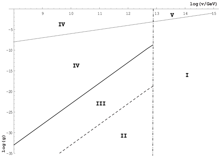
Figure 3: We show the various regions according to the $\theta$ production mechanism in the early universe. With this objective, we display the lines: $T_{\ast}=v$ (dotted line), $T_{\ast}=T_{end}$ (solid line), $n_{th}=n_{non-th}$ (dashed line) and $v=v_{th}$ (dot-dashed line). In (I) and (V) there is only non-thermal production. In (II) and (III) there are non-thermal and thermal processes that generate $\theta$, in (II) non-thermal dominates while in (III), it is thermal production that dominates. In (IV) there is thermally and non-thermally produced $\theta$s, but the last are thermalized. In (V), we have not a general formula for predicting $n_{non-th}$.

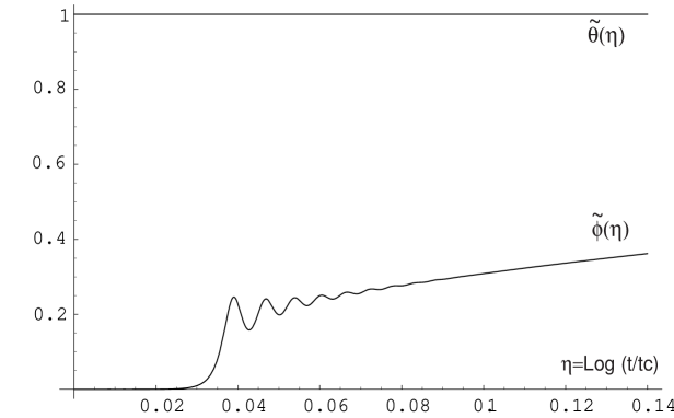
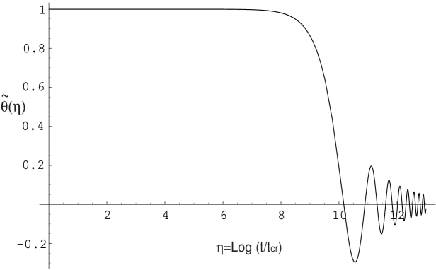
Figure 8: Evolution of the normalized fields $\tilde{\theta}$ and $\tilde{\phi}$ as a function of $\eta=\log(t/t_{cr})$ with $t_{cr}$ defined in (38). We see how $\tilde{\phi}$ evolves first while $\tilde{\theta}$ remains constant (a), and how $\tilde{\theta}$ finally oscillates (b). Notice the (logarithmic) time scales. For this numerical simulation we chose: $v=10^{11}$, $\lambda=10^{-2}$ and $g=10^{-8}$.

References

- (1) See for instance T. Banks, Physicalia 12, 19 (1990), and references therein.
-
(2)
S. B. Giddings and A. Strominger,
Nucl. Phys. B 307, 854 (1988).
S. R. Coleman, Nucl. Phys. B 310, 643 (1988).
G. Gilbert, Nucl. Phys. B 328, 159 (1989). - (3) G. B. Gelmini, S. Nussinov and T. Yanagida, Nucl. Phys. B 219, 31 (1983).
-
(4)
S. Weinberg,
Phys. Rev. Lett. 40, 223 (1978).
F. Wilczek, Phys. Rev. Lett. 40, 279 (1978). - (5) For a comprehensive review, see G. G. Raffelt, Stars As Laboratories For Fundamental Physics (University of Chicago Press, Chicago, 1996).
-
(6)
J. Preskill, M. B. Wise and F. Wilczek,
Phys. Lett. B 120, 127 (1983).
L. F. Abbott and P. Sikivie, Phys. Lett. B 120, 133 (1983).
M. Dine and W. Fischler, Phys. Lett. B 120, 137 (1983). -
(7)
A. Vilenkin and E. P. S. Shellard, Cosmic Strings and other
Topological Defects (Cambridge University Press, Cambridge, 1994).
A. Vilenkin and A. E. Everett, Pseudogoldstone Phys. Rev. Lett. 48, 1867 (1982). - (8) E. K. Akhmedov, Z. G. Berezhiani, R. N. Mohapatra and G. Senjanovic, Phys. Lett. B 299, 90 (1993)
-
(9)
C. T. Hill and G. G. Ross,
Phys. Lett. B 203, 125 (1988).
C. T. Hill and G. G. Ross, Nucl. Phys. B 311, 253 (1988). -
(10)
M. Lusignoli, A. Masiero and M. Roncadelli,
Phys. Lett. B 252, 247 (1990).
S. Ghigna, M. Lusignoli and M. Roncadelli, Phys. Lett. B 283, 278 (1992).
D. Grasso, M. Lusignoli and M. Roncadelli, Phys. Lett. B 288, 140 (1992). -
(11)
C. T. Hill, D. N. Schramm and J. N. Fry,
Comments Nucl. Part. Phys. 19, 25 (1989).
A. K. Gupta, C. T. Hill, R. Holman and E. W. Kolb, Phys. Rev. D 45, 441 (1992).
J. A. Frieman, C. T. Hill and R. Watkins, Phys. Rev. D 46, 1226 (1992).
J. A. Frieman, C. T. Hill, A. Stebbins and I. Waga, Phys. Rev. Lett. 75, 2077 (1995) [arXiv:astro-ph/9505060]. - (12) D. Kazanas, R. N. Mohapatra, S. Nasri and V. L. Teplitz, arXiv:hep-ph/0403291.
-
(13)
R. N. Mohapatra and X. Zhang,
Phys. Rev. D 49, 1163 (1994) [Erratum-ibid. D 49,
6246 (1994)].
R. N. Mohapatra and A. Riotto, Phys. Rev. Lett. 73, 1324 (1994). - (14) C. L. Bennett et al., Astrophys. J. Suppl. 148, 1 (2003).
- (15) E. W. Kolb and M. S. Turner, “The Early Universe,” Redwood City, USA: Addison-Wesley (1990) 547 p. (Frontiers in physics, 69).
-
(16)
R. L. Davis,
Phys. Lett. B 180, 225 (1986).
R. A. Battye and E. P. S. Shellard, Phys. Rev. Lett. 73, 2954 (1994) [Erratum-ibid. 76, 2203 (1996)] [arXiv:astro-ph/9403018].
R. L. Davis, Phys. Rev. D 32, 3172 (1985).
R. A. Battye and E. P. S. Shellard, Nucl. Phys. B 423, 260 (1994) [arXiv:astro-ph/9311017].
M. Yamaguchi, M. Kawasaki and J. Yokoyama, Phys. Rev. Lett. 82, 4578 (1999) [arXiv:hep-ph/9811311]. -
(17)
D. Harari and P. Sikivie,
Phys. Lett. B 195, 361 (1987).
C. Hagmann and P. Sikivie, Nucl. Phys. B 363, 247 (1991).
C. Hagmann, S. Chang and P. Sikivie, Phys. Rev. D 63, 125018 (2001) [arXiv:hep-ph/0012361]. - (18) M. S. Turner, Phys. Rev. Lett. 59, 2489 (1987) [Erratum-ibid. 60, 1101 (1988)].
- (19) E. Masso, F. Rota and G. Zsembinszki, Phys. Rev. D 66, 023004 (2002).
- (20) K. Hagiwara et al. [Particle Data Group Collaboration], Phys. Rev. D 66, 010001 (2002).
- (21) E. Masso and R. Toldrà, Phys. Rev. D 60, 083503 (1999).
- (22) M. T. Ressell and M. S. Turner, Bull. Am. Astron. Soc. 22, 753 (1990).
- (23) R. A. Sunyaev and Y. B. Zeldovich, Ann. Rev. Astron. Astrophys. 18, 537 (1980).
- (24) E. Masso and R. Toldrà, Phys. Rev. D 55, 7967 (1997) [arXiv:hep-ph/9702275].
- (25) S. Sarkar, Rept. Prog. Phys. 59, 1493 (1996).
- (26) R. J. Scherrer and M. S. Turner, Phys. Rev. D 31, 681 (1985).
- (27) R. J. Scherrer and M. S. Turner, Astrophys. J. 331, 19 (1988) [Astrophys. J. 331, 33 (1988)].
- (28) For a recent review, see E. Masso, Nucl. Phys. Proc. Suppl. 114, 67 (2003) [arXiv:hep-ph/0209132].
- (29) R. D. Peccei, arXiv:hep-ph/0009030.
- (30) See, for example, M. Quiros, arXiv:hep-ph/9901312.
- (31) L. Dolan and R. Jackiw, Phys. Rev. D 9, 3320 (1974).