ROM2F/2004/13

Layered Higgs Phase as a Possible Field Localisation on a Brane

P. Dimopoulos^(a) and K. Farakos^(b)

^(a) INFN-Rome2 Universita di Roma ’Tor Vergata’
Dipartimento di Fisica I-00133, Rome, Italy

^(b) Physics Department, National Technical University
15780 Zografou Campus, Athens, Greece

So far it has been found by using lattice techniques that in the anisotropic five–dimensional Abelian Higgs model, a layered Higgs phase exists in addition to the expected five–dimensional one. The exploration of the phase diagram has shown that the two Higgs phases are separated by a phase transition from the confining phase. This transition is known to be first order. In this paper we explore the possibility of finding a second order transition point in the critical line which separates the first order phase transition from the crossover region. This is shown to be the case only for the four–dimensional Higgs layered phase whilst the phase transition to the five–dimensional broken phase remains first order. The layered phase serves as the possible realisation of four–dimensional spacetime dynamics which is embedded in a five–dimensional spacetime. These results are due to gauge and scalar field localisation by confining interactions along the extra fifth direction.

1 Introduction - Motivation

Since the mid eighties lattice gauge models with anisotropic couplings defined in higher D-dimensional spaces have been proposed. These models may exhibit, through a phase transition, a phase which is coulombic in (D-1) dimensions and shows confinement along the remaining dimension. In fact, this was the result of Fu and Nielsen using mean field techniques in a five-dimensional pure U(1) gauge theory with anisotropic couplings [1]. This new phase was called layered.

The Monte–Carlo analysis which followed [2] supported the mean field results and helped to get a more precise picture of the phase diagram [3]. Also in [4] the orders of the phase transitions have been analysed .

In addition, as it may have been expected, the consideration of the interaction with a scalar particle leads to a richer phase diagram. Actually, the exploration of the phase diagram of the model for various sets of lattice parameters values provides strong evidence that the layer phase is stable and it appears either in a Higgs phase for the U(1) case [7, 8], or in a Coulomb phase for a SU(2) adjoint Higgs model [11].

Since gauge theories defined on a $D>4$ spacetime are known to be non–renormalisable an explicit cut–off $\Lambda$ has to be introduced [12]. Therefore the theory is to be considered as an effective theory which emerges from a more fundamental renormalisable theory (for example the string theory). For the U(1) gauge field the introduction of the cut–off $\Lambda$ leads to the admission of the strong coupling phase to be the interesting phase for the five–dimensional theory. As a consequence the lattice methods have to be used as the unavoidable non–perturbative tool for the study of the system.

Up to now the Monte–Carlo results show that the transition between the five dimensional strong coupling phase and the layered Higgs phase is first order. A multilayer structure arises which supports the idea of the confinement along the extra dimension [8, 11]. A crucial question may arise: is there any possibility for this phase transition to be of second order? We work on this possibility and we look for a second order ending point along the first order critical line . This would give evidence for the layer mechanism to be more realistic and useful in scenarios concerning the localisation of the fields on the four–dimensional subspace.

Before proceeding to the lattice model let us present the action of the U(1)–Higgs model in five dimensions which in principle could inspire the lattice action used in the sequel for the numerical simulation.

We assume a five dimensional anti de Sitter space ($\mbox{AdS}_{5}$) with one warped extra dimension. In general the metric reads:

$$ds^{2}=\alpha^{2}(z)[dx_{0}^{2}-d\vec{x}^{2}]-dz^{2}$$ (1.1)

We consider $\eta_{\mu\nu}$ to be the four dimensional Minkowski metric and $\alpha(z)$ the warp factor. We do not need to define explicitly the form of the warp factor. We only require that it goes to zero as $z\rightarrow\infty$ ([16],[17], [18], [19]). Hence the five–dimensional metric is written:

$$g^{MN}=(\displaystyle{\frac{1}{\alpha^{2}(z)}}\eta^{\mu\nu},-1)$$ (1.2)

We consider now that in such a space we define a five dimensional Abelian Higgs model, the action of which reads:

$$S = S_{\mbox{gauge}}+S_{\mbox{scalar}}$$ (1.3)

$$= -\displaystyle{\frac{1}{4g_{5}^{2}}}\int d^{5}x\sqrt{g}~{}~{}F_{MN}F_{KL}g^{MK}g^{NL}+\int d^{5}x\sqrt{g}~{}~{}\left[D_{M}\Phi^{*}D_{N}\Phi g^{MN}-V(\Phi)\right]$$

$$= \int d^{4}xdz\left[-\displaystyle{\frac{1}{4g_{5}^{2}}}F_{\mu\nu}F_{\kappa\lambda}\eta^{\mu\kappa}\eta^{\nu\lambda}-\displaystyle{\frac{\alpha^{2}(z)}{2g_{5}^{2}}}F_{\mu 5}F_{\nu 5}\eta^{\mu\nu}\right]+$$

$$+ \int d^{4}xdz\left[\alpha^{2}(z)D_{\mu}\Phi^{*}D_{\nu}\Phi\eta^{\mu\nu}-\alpha^{4}(z)D_{z}\Phi^{*}D_{z}\Phi-\alpha^{4}(z)V(\Phi)\right]$$

We note that the upper case indices refer to the 5–D space, $M,N,K,L=0,...,4$ and the lower case Greek ones to the 4–D space i.e. $\mu,\nu,\kappa,\lambda=0,...,3$. It is obvious that the scalar field $\Phi$ depends on the five dimensional space $(x,z)$. Then we use the rescaling: $\alpha(z)\Phi=\varphi$ for the scalar field. In the rather general case where the quartic scalar potential is considered, the scalar action takes the form:

$$S_{\mbox{scalar}}=\int d^{4}xdz\left[D_{\mu}\varphi^{*}D^{\mu}\varphi-\alpha^{2}(z)D_{z}\varphi^{*}D_{z}\varphi-M(z)^{2}\varphi^{*}\varphi-\lambda(\varphi^{*}\varphi)^{2}\right]$$ (1.4)

where $M^{2}(z)=\alpha^{2}(z)m^{2}+[\alpha^{\prime}(z)]^{2}+\frac{1}{2}[\alpha^{2}(z)]^{{}^{\prime\prime}}$ .

It is a trivial matter for the action to be analytically continued to the Euclidean space from which the lattice action can be defined after following the usual methods for discretization. Therefore we take:

$$S_{\small L} = S_{\mbox{gauge}}+S_{\mbox{scalar}}$$ (1.5)

$$= \beta_{g}\sum_{x}\sum_{1\leq\mu<\nu\leq 4}(1-\cos U_{\mu\nu}(x))+\sum_{x}\sum_{1\leq\mu\leq 4}\beta_{g}^{\prime}~{}(1-\cos U_{\mu 5}(x))$$

$$+ \beta_{h}\sum_{x}\sum_{1\leq\mu\leq 4}[\varphi_{\small L}(x)-U_{\hat{\mu}}(x)\varphi_{L}(x+a\hat{\mu})]^{*}[\varphi_{\small L}(x)-U_{\hat{\mu}}(x)\varphi_{\small L}(x+a\hat{\mu})]$$

$$+ \beta_{h}^{\prime}\sum_{x}[\varphi_{L}(x)-U_{\hat{5}}(x)\varphi_{L}(x+a\hat{5})]^{*}[\varphi_{\small L}(x)-U_{\hat{5}}(x)\varphi_{\small L}(x+a\hat{5})]$$

$$+ \sum_{x}m^{2}_{L}\varphi^{*}_{\small L}(x)\varphi_{\small L}(x)+\beta_{R}(\varphi^{*}_{\small L}(x)\varphi_{\small L}(x))^{2}],$$

We denote by $\varphi_{L}(x)$ the lattice scalar field and

$$U_{\mu\nu}(x) = U_{\mu}(x)U_{\nu}(x+a\hat{\mu})U_{\mu}^{\dagger}(x+a\hat{\nu})U_{\nu}^{\dagger}(x)$$

$$U_{\mu 5}(x) = U_{\mu}(x)U_{5}(x+a\hat{\mu})U_{\mu}^{\dagger}(x+a\hat{5})U_{5}^{\dagger}(x)$$ (1.6)

are the plaquettes on the four–dimensional space and along the fifth direction respectively The U’s are the links for the gauge field on the lattice . They are explicitly given by: $U_{M}=e^{iaA_{M}}~{}~{}~{}(\mbox{with}~{}~{}M=1,...,5)$. The primed couplings refer to the interactions along the extra dimension. Moreover as it can be noticed from the corresponding continuous action, the couplings obey certain relationships, which depend on the warp factor . Hence we have:

$$\beta_{g}^{{}^{\prime}}=\alpha^{2}(x_{T})\beta_{g},~{}~{}~{}~{}\beta_{h}^{{}^{\prime}}=\alpha^{2}(x_{T})\beta_{h},~{}~{}~{}~{}\lambda=\frac{4\beta_{R}a}{\beta_{h}^{2}}$$ (1.7)

$$a^{2}M^{2}(x_{T})=\frac{2}{\beta_{h}}m^{2}_{L}$$ (1.8)

Therefore due to the assumed form for the warp factor the interactions for both the gauge and scalar fields are strongly coupled along the extra direction.
Since a brane is defined as any three dimensional submanifold to which ordinary matter is trapped [20] so that it can not escape to the bulk, a possible realisation of the trapping mechanism is to assume the existence of confinement along the extra dimension. On the lattice this situation can be realised using a lattice model with anisotropic couplings. This is sufficient to lead to the formation of the layered phase through a phase transition. In our context we consider this layered phase on the lattice as a possible paradigm on how a localisation of the fields, obeying to non-perturbative interactions, may be carried out on the brane due to confining interactions in the bulk.

In this paper we study a simplified realisation of the lattice action given by Eq. (1.9) below. This is inspired by Eq. (1.7) i.e. to set the fifth (transverse) direction couplings to a strong coupling regime while we neglect the explicit role of the warp factor in the lattice action. Therefore the lattice action (which leads to the five dimensional Higgs model in the naive continuum limit ([7], [8]) ) reads in standard notation:

$$S_{\small L} = S_{\mbox{gauge}}+S_{\mbox{scalar}}$$ (1.9)

$$= \beta_{g}\sum_{x}\sum_{1\leq\mu<\nu\leq 4}(1-\cos U_{\mu\nu}(x))+\sum_{x}\sum_{1\leq\mu\leq 4}\beta_{g}^{\prime}~{}(1-\cos U_{\mu 5}(x))$$

$$+ \beta_{h}\sum_{x}{\rm Re}[4\varphi^{*}_{\small L}(x)\varphi_{\small L}(x)-\sum_{1\leq\mu\leq 4}\varphi^{*}_{\small L}(x)U_{\hat{\mu}}(x)\varphi_{\small L}(x+a\hat{\mu})]$$

$$+ \sum_{x}\beta_{h}^{\prime}~{}{\rm Re}[(\varphi^{*}_{\small L}(x)\varphi_{\small L}(x)-\varphi^{*}_{\small L}(x)U_{\hat{5}}(x)\varphi_{\small L}(x+a\hat{5})]$$

$$+ \sum_{x}[(1-2\beta_{R}-4\beta_{h}-\beta_{h}^{\prime})\varphi^{*}_{\small L}(x)\varphi_{\small L}(x)+\beta_{R}(\varphi^{*}_{\small L}(x)\varphi_{\small L}(x))^{2}],$$

Apart from the resulting simplicity in the context of the phase diagram analysis, a connection of this work with previous studies of the layered phase can be achieved. Moreover our impression is that the full lattice model is likely to produce physically similar results with the present simplified version. This was also the case for the pure U(1) gauge model. The ’static’ representation of the model for which the gauge couplings were fixed by hand gave equivalent resuts with the model in which the warp factor was used for the scaling of the gauge couplings [4].

2 The order parameters and the choice of couplings

We study the abelian Higgs model on the lattice by using numerical methods. The action is given explicitly by Eq. (1.9). We define five order parameters, making also the distinction between space–like and transverse–like ones. These are the following:

$$\mbox{ Space--like Plaquette:}\hskip 8.5359ptP_{S}\equiv<\frac{1}{6N^{5}}\sum_{x}\sum_{1\leq\mu<\nu\leq 4}\cos U_{\mu\nu}(x)>$$

$$\mbox{ Transverse-like~{}Plaquette:}\hskip 8.5359ptP_{T}\equiv<\frac{1}{4N^{5}}\sum_{x}\sum_{1\leq\mu\leq 4}\cos U_{\mu 5}(x)>$$

$$\mbox{Space-like~{}Link:}\hskip 8.5359ptL_{S}\equiv<\frac{1}{4N^{5}}\sum_{x}\sum_{1\leq\mu\leq 4}\cos(\chi(x+\hat{\mu})+A_{\hat{\mu}}(x)-\chi(x))>$$

$$\mbox{ Transverse-like~{}Link:}\hskip 8.5359ptL_{T}\equiv<\frac{1}{N^{5}}\sum_{x}\cos(\chi(x+\hat{5})+A_{\hat{5}}(x)-\chi(x))>$$

$$\mbox{Higgs~{}field~{}measure~{}squared:}\hskip 8.5359ptR^{2}\equiv\frac{1}{N^{5}}\sum_{x}\rho^{2}(x)$$

We have assumed the polar form for the scalar field, i.e. $\varphi_{L}=\rho(x)e^{i\chi(x)}$.

In [8] this model has been already studied and a first exploration for the phase diagram is available. In that work, since the parameter space is very large, consisting of five lattice parameters,the choice has been made to fix $\beta_{g}$ to 0.5, $\beta_{h}^{\prime}$ to 0.001 and consider two values of $\beta_{R}$ (0.1 and 0.01) and explore the parameter space ($\beta_{g}^{\prime}$, $\beta_{h}$). Under these conditions the analysis of the order parameters defined above yielded a phase diagram consisting of the three expected phases which are the confining phase ($S$), the Coulomb phase ($C_{5}$) and the Higgs phase ($H_{5}$) each of them defined in five dimensions. In addition a fourth phase is present: a Higgs phase in four dimensions ($H_{4}$) (see Fig.1). The distinction between $H_{4}$ and $H_{5}$ can be achieved due to the different behaviour of the transverse–like order parameters within the two phases. Details and conclusions on the existence of this layer Higgs phase can be found in [8]. Let us refer also that the identification for the order of the phase transitions was possible and has lead to the conclusion that (for the two values of $\beta_{R}$ used) both $H_{4}$, $H_{5}$ are separated from the confining phase by a first order phase transition. We reproduce the phase diagram for $\beta_{R}=0.1$ as it was depicted in [8] (Fig.1).

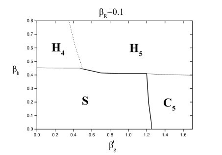
Figure 1: Phase diagram of the 5-D Abelian Higgs Model with the space–like gauge coupling set to the strong coupling $\beta_{g}=0.5$ (taken from [8]).

3 Searching for a second order phase transition

At this point the question arises whether it could be possible for the $H_{4}$ layer phase to appear via a second order phase transition. Following [8], we consider the system being in the confining regime by setting $\beta_{g}=0.5$ and fixing $\beta^{\prime}_{h}$ to the very small value 0.001. We expect the phase transitions to the Higgs phases to be weaker as the Higgs self coupling $\beta_{R}$ increases. We explore the order of the $S-H_{4}$ phase transition by setting the transverse gauge coupling $\beta^{\prime}_{g}$ to 0.2 while we increase $\beta_{R}$. In advance, it should be noted that, as we move to larger values of $\beta_{R}$, the relative positions of the phases in the phase diagram are substantially similar to what is shown in Fig.1 for $\beta_{R}=0.1$. So, setting $\beta^{\prime}_{g}$ to 0.2, we always explore the $S-H_{4}$ phase transition.

In the sequel we give strong evidence that, the $S-H_{4}$ first order phase transition line ends at a second order point followed by a crossover region. At the same moment the $S-H_{5}$ phase transition remains first order. This additional fact confirms the special nature of the four dimensional layer Higgs phase.

We give now information for the simulating process. We used a 4–hit metropolis algorithm for the updating of the fields. In addition we implemented the global radial algorithm and the overrelaxation algorithm for the updating of the Higgs field. We used four lattice volumes, $8^{5}$, $10^{5}$, $12^{5}$, $14^{5}$, and we performed 20000–30000 measurements for each point which we analyzed in the parameter space. We studied a large number of $\beta_{R}$ values before concentrating our study to the interval $[0.140,0.165]$ in which the first order phase transition turns to be a weaker one before it passes to the crossover region.

In the subsequent paragraphs we present our results which are based upon using the hysteresis loop technique, the finite volume size scaling, the susceptibility and the study of the correlation functions for the Higgs field measure squared.

3.1 Hysteresis loop technique results

The first tool for the exploration of the phase diagram with $\beta_{R}$ is the hysteresis loop technique. Although this technique gives results that have to be taken into account with caution quantitatively, nevertheless they prove to be very useful as qualitative ones. To this end we use the hysteresis loop results as a general guide to get a crude estimate on the $\beta_{R}$ interval within which the phase transition is converted from a first order to a higher order one. In Fig.2 we depict the hysteresis loop results for the four –dimensional gauge invariant quantity $L_{S}$ and for four values of $\beta_{R}$, namely $\beta_{R}=0.143,0.149,0.153,0.160$. The lattice volume in this example is $8^{5}$. One can see from the figure that while there is a well formed loop for $\beta_{R}=0.143$ indicating a first order phase transition, this changes to a smaller one for $\beta_{R}=0.149$, and it seems to disappear for $\beta_{R}=0.153$. Although this value should not be taken too seriously, one should keep in mind that around the value $\beta_{R}=0.153$ a weaker phase transition is still present. Furthermore we have to mention that the transverse link quantity, $L_{T}$, (not shown in the figure) remains almost unaffected by the phase transition, being stuck to a very small value close to zero (for details see [8]).

Figure 2: Hysteresis loops showing that the loop for the link–space order parameter disappears for $\beta_{R}$ values bigger than 0.153.

In Fig. 3 we give an example of the different phase transition orders of the $S-H_{4}$ and $S-H_{5}$ transitions, both for $\beta_{R}=0.158$ and lattice volume $8^{5}$. In Fig.3a we present the hysteresis loop results on $P_{S}$ and $P_{T}$ for $\beta^{\prime}_{g}=0.20$. The behaviour of $P_{S}$ indicates a phase transition though a smooth one since there is no hysteresis loop, while the $P_{T}$ is almost constant and equals 0.1, in accord with the strong coupling prediction $\beta_{g}^{\prime}/2$. This figure should be compared with the Fig.3b, which refers to $\beta^{\prime}_{g}=0.80$. The hysteresis loop results shows a very strong first order phase transition, exhibited by both $P_{S}$, $P_{T}$. This behaviour refers to the $S-H_{5}$ phase transition. Figures 3c and 3d show the behaviour for $R^{2}$ which illustrates the fact that for both cases the system passes to a broken phase. In other words, increasing $\beta{{}_{g}}^{\prime}$ one finds two different Higgs phases (see for example Fig.1), a four–dimensional and a five–dimensional one both separated from the five–dimensional confining phase by phase transitions of different orders.

Figure 3: Characteristic examples showing the obviously different order of the phase transition for the cases $S-H_{4}$ and $S-H_{5}$ at the same value of $\beta_{R}$, for two different values of $\beta_{g}^{\prime}$.

3.2 Finite volume size scaling

As it has been discussed in [8] one of the main features of the $S-H_{4}$ phase transition is the multi–layer structure. This means that since the system undergoes a transition to a four–dimensional phase rather than a five dimensional one, some special signal should appear. Besides a first order phase transition this consists of a multipeak structure in the finite lattice volume histograms for the gauge invariant observables, instead of the expected behaviour of the two-peak structure. Furthermore it has been shown that every space–like gauge invariant quantity defined on each space–like volume (i.e. a four–dimensional layer) ’feels’ the phase transition for different pseudocritical values of the lattice parameters. Since this is a consequence of the finite lattice volume used for Monte–Carlo simulations in combination with the four–dimensional dynamics when the layer phase arises, we justify the choice of analysing the results on the four–dimensional subspace.

In Fig.4 we depict the histograms of the Higgs field measure squared, $R^{2}$ for $\beta^{\prime}_{g}=0.20$ and three values of $\beta_{R}$. All the three histograms refer to $\beta_{h}$ values in the critical region. The lattice volume in this figure is $14^{5}$. The $R^{2}$ histograms refer to four–dimensional (space–like) volume. The two peak structure is more pronounced for the smaller value of $\beta_{R}$ (i.e. 0.153), where the two peaks are totally separated. For $\beta_{R}=0.155$ the two peak structure is less emphasised while for $\beta_{R}=0.158$ it has already disappeared. In order for someone to use this method with more safety the lattice volume dependence of the two peak structure should be taken into account. This is provided in Fig.5 . In Fig.5a it is easily seen that the two peaks become well separated as the lattice length increases from $10$ to $14$ which serves as an indication of a first order phase transition for the case of $\beta_{R}=0.153$. This has to be compared with the really inversed behaviour for $\beta_{R}=0.158$ shown in Fig.5c. The $\beta_{R}=0.155$ case, Fig.5b, for which the peak separation does not change significantly as the lattice length goes from $10$ to $14$, gives an estimate of a first order phase transition becoming much weaker and probably of higher order.

Figure 4: Histograms of $R^{2}$ over a space–like volume for three values of $\beta_{R}=0.153,0.155,0.158$ and lattice length $N=14$.

Figure 5: The histograms for $R^{2}$ as the lattice length increases for the three values of $\beta_{R}=0.153,0.155,0.158$.

Let us now present more quantitative results by giving the results for the susceptibility of $R^{2}$ on the layers for various values of $\beta_{R}$. This is defined by:

$$S(R^{2})=V_{s}(<(R^{2})^{2}>-<R^{2}>^{2})$$

where $V_{s}$ denotes the space–like lattice volume. The results are depicted in Fig.6. The errors have been calculated by using the Jackknife method. It is known that a first order phase transition is signalled by a linear increase of the maximum of the susceptibility with the volume. This is actually the case for $\beta_{R}=0.149~{}\mbox{and}~{}0.153$. The situation changes for $\beta_{R}=0.155$ where the linear behaviour is apparently absent. In addition, for the bigger values $\beta_{R}=0.158~{}\mbox{and}~{}0.160$ there is not a clear increase with the volume. This case corresponds to a crossover behaviour. Therefore, the conclusion is that in the vicinity of $\beta_{R}=0.155$ we meet with the well known situation, where a first order phase transition line ends to a second order phase transition point followed by a crossover.

Figure 6: The susceptibility versus the space–like volume for five values of $\beta_{R}$ in the critical $\beta_{R}$ region.

3.3 Correlation functions

In this section we present the behaviour of two correlation functions, one defined on the whole five–dimensional space and the other on the space–like, four–dimensional one. These correlation functions involve the Higgs field measure squared $R^{2}$, defined in section 2. The definition of the correlation functions is given by:

$$C_{S,T}(n)=\sum_{i}\frac{<(R^{2})_{i}(R^{2})_{i+n}>-<(R^{2})_{i}>^{2}}{<(R^{2})_{i}^{2}>-<(R^{2})_{i}>^{2}}$$ (3.10)

where $n$ takes values from 1 to $N$ (i.e. the lattice size). The indices $S$ and $T$ are used to distinguish the correlators. The one defined in the transverse direction is noted with the index $T$. The other defined in the space–like volume is denoted with $S$.

Figure 7: The space–like and time–like correlation functions for $L=14$ and for three values of $\beta_{R}=0.155,~{}0.158,~{}0.160$, in the region of $\beta_{h}$ where the susceptibilities show a peak.

The results for the two correlators are radically different. An example of our results is shown in Fig.7. This refers to the case of $N=14$ lattice size for three values of $\beta_{R}$. We see that while $C_{T}$ decreases very fast, reaching zero and fluctuating around it, $C_{S}$ takes values different from zero. This serves as a clear evidence that a layered phase is formed. The layers are decoupled as a consequence of the strong coupling imposed on the transverse direction, which has the implication of vanishing $C_{T}$. Moreover the rather reasonable behaviour of $C_{S}$ shows that inside the layers a four dimensional dynamics is still met as it might be expected.

$$\begin{array}[]{ccccccc}\hline\cr\\ \mbox{Lattice size}&&\beta_{R}=0.155&&\beta_{R}=0.158&&\beta_{R}=0.160\\ \hline\cr\\ 10&&0.145(3)&&0.165(4)&&0.181(4)\\ 12&&0.112(3)&&0.137(3)&&0.167(7)\\ 14&&0.090(3)&&0.131(6)&&0.152(7)\\ \hline\cr\\ \end{array}$$

Table 1: The masses in lattice units. We observe that for $L=14$ and $\beta_{R}=0.155$ the value for the mass parameter has decreased by a factor of 1.7 in comparison with the $\beta_{R}=0.160$ corresponding value.

Another very interesting feature of the $C_{S}$ correlation function is that as the $\beta_{R}$ value decreases the curve becomes more flat. We should note that in the case of a second order phase transition and for infinite volume this should be really flat. This is a fact corresponding to infinite correlation length or vanishing mass for the lightest scalar mode. In other words, by adjusting the $\beta_{h}$ value into the critical region we might expect a mass behaviour of the type $m_{s}\propto(\beta_{R}-\beta_{R}^{c})^{\nu}$. The light scalar mass calculation can be achieved by using a fit of the form $const\times\cosh(m_{s}(x-N/2))$ to the correlation functions $C_{S}$. The parameter $m_{s}$ is the dimensionless mass parameter of the scalar mode. An example of the fits is shown in Fig.7. The results for $m_{s}$ for the cases considered are shown in Table 1. From that Table and for the largest lattice size used we can see that $m_{s}$ decreases by a factor of 1.7 between $\beta_{R}=0.160$ and 0.155. A more clear signal for the vanishing $m_{s}$ would require bigger volumes and still higher computer time. Nevertheless, after considering the previous analysis on susceptibility combined with the results from the study of the correlations, we are justified to estimate that at $\beta_{R}=0.155(2)$ a second order phase transition point should be expected.

4 Conclusions

We believe that we have serious evidence that the five–dimensional Abelian Higgs model with strong coupled interactions along the fifth (transverse) direction reveals a four–dimensional dynamics with broken gauge symmetry. This occurs via a second order phase transition. The existence of the layered phase can be considered as a realisation for the localisation of the gauge and scalar fields for models defined in a higher dimensional space with the extra dimensions being warped. Although the lattice volumes and the computer power available is not conclusive for the second order critical point (so that the calculation of critical exponents is out of consideration for the moment), our results provide an estimate for the value of the Higgs self coupling at which the line of the first order transition line ends in a second order transition point along the four–dimensional space.

5 Acknowledgements

We thank A. Kehagias and G. Koutsoumbas for reading and comments on the manuscript. We also wish to thank K. Bachas, M. Giovannini for useful discussions. Thanks are also due to the Computer Center of the NTUA for the computer time allocated. The work of P.D. is partially supported by ”Thales” project of NTUA and the ”Pythagoras” project of the Greek Ministry of Education.

References

- [1] Y.K. Fu and H.B. Nielsen, Nucl. Phys. B 236, 167 (1984); Nucl. Phys. B236, 127 (1985).
- [2] D. Berman and E. Rabinovici, Phys. Lett. B157 292 (1985).
- [3] C.P. Korthals-Altes, S. Nicolis and J. Prades, Phys. Lett. B316 339 (1993) [hep-lat/9306017]; A. Hulsebos, C.P. Korthals-Altes and S. Nicolis, Nucl. Phys. B450 437 (1995) [hep-th/9406003].
- [4] P. Dimopoulos, K. Farakos, A. Kehagias and G. Koutsoumbas, Nucl.Phys.B617:237-252,2001 [hep-th/0007079];
- [5] S. Ejiri, J. Kubo and M. Murata, Phys.Rev.D62:105025,(2000) [hep-ph/0006217]; S. Ejiri, S. Fujimoto and J. Kubo, Phys.Rev.D66:036002,(2002) [hep-lat/0204022].
- [6] K. Farakos, P. de Forcrand, C.P. Korthals Altes, M. Laine and M. Vettorazzo,
- [7] P. Dimopoulos, K. Farakos, G. Koutsoumbas, C.P. Korthals-Altes, S. Nicolis, JHEP 02(005) (2001) [hep-lat/0012028];
- [8] P. Dimopoulos, K. Farakos and S. Nicolis, Eur.Phys.J.C24:287-296,2002, [hep-lat/0105014].
- [9] M.Laine, H.B.Meyer, K.Rummukainen and M.Shaposhnikov, Effective Gauge Theories on Domain Walls via Bulk Confinement? [hep-ph/0404058].
- [10] G.R. Dvali and M.A. Shifman, Phys.Lett.B396:64 (1997), Erratum-ibid.B407:452 (1997) [hep-th/9612128].
- [11] P. Dimopoulos, K. Farakos and G. Koutsoumbas, Phys.Rev.D65:074505,2002 [hep-lat/0111047].
- [12] K.R. Dienes, E. Dudas and T. Gharghetta, Nucl. Phys. B537 (1999) 47, [hep-ph/9806292].
- [13] J.L.Alonso et. al. Nucl.Phys. B405 (1993) 574, [hep-lat/9210014]
- [14] K.Kajantie, M.Laine, K.Rummukainen and M.Shaposhnikov, Phys.Rev.Lett. 77 2887 (1996) [hep-ph/9605288]; K.Rummukainen, M.Tsypin, K.Kajantie, M.Laine and M.Shaposhnikov, Nucl. Phys. B532 283 (1998) [hep-lat/9805013]
- [15] A. Hart, O. Philipsen, J.D. Stack and M. Teper, Phys.Lett. B396 217 (1997)[hep-lat/9612021].
- [16] L. Randall and R. Sundrum, Phys. Rev. Lett. 83 (1999) 4690, [hep-th/9906064]; L. Randall and R. Sundrum, Phys. Rev. Lett. 83 (1999) 3370, [hep-th/9905221].
- [17] A. Kehagias, Phys. Lett. B469 (1999) 123, [hep-th/9906204]; A. Kehagias and K. Tamvakis, Phys. Lett. B504 (2001) 38, [hep-th/0010112].
- [18] M. Giovannini, Phys. Rev. D64 (2001) 124004, [hep-th/0107233]; Phys.Rev. D65 (2002) 124019, [hep-th/0204235].
- [19] M.Shaposhnikov and P.Tinyakov, Phys.Lett. B515 (2001) 442-446, [hep-th/0102161]; M.Laine, H.B.Meyer, K.Rummukainen and M.Shaposhnikov, JHEP 0301 (2003) 068 [hep-ph/0211149].
- [20] V.A. Rubakov, Usp.Fiz.Nauk 171 913-938 (2001), [hep-ph/0104152]