Off mass shell dual amplitude with Mandelstam analyticity

Abstract

A model for the $Q^{2}$-dependent dual amplitude with Mandelstam analyticity (DAMA) is proposed. The modified DAMA (M-DAMA) preserves all the attractive properties of DAMA, such as its pole structure and Regge asymptotics, and leads to a generalized dual amplitude $A(s,t,Q^{2})$. This generalized amplitude can be checked in the known kinematical limits, i.e. it should reduce to the ordinary dual amplitude on mass shell, and to the nuclear structure function when $t=0$. In such a way we complete a unified "two-dimensionally dual" picture of strong interaction JM0dama ; JM1dama ; JMfitnospin ; JMfitspin . By comparing the structure function $F_{2}$, resulting from M-DAMA, with phenomenological parameterizations, we fix the $Q^{2}$-dependence in M-DAMA. In all studied regions, i.e. in the large and low $x$ limits as well as in the resonance region, the results of M-DAMA are in qualitative agreement with the experiment.

1 Introduction

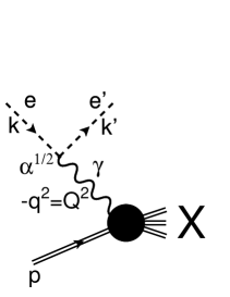
5mm normal

Figure 1: Kinematics of deep inelastic scattering.

About thirty years ago Bloom and Gilman BG observed that the prominent resonances in inelastic electron-proton scattering (see Fig. 1) do not disappear with increasing photon virtuality $Q^{2}$ with respect to the "background" but instead fall at roughly the same rate as background. Furthermore, the smooth scaling limit proved to be an accurate average over resonance bumps seen at lower $Q^{2}$ and $s$, this is so called Bloom-Gilman or hadron-parton duality.

For the inclusive $e^{-}p$ reaction we introduce virtuality $Q^{2}$, $Q^{2}=-q^{2}=-(k-k^{\prime})^{2}\geq 0$, and Bjorken variable $x$. These variables $x$, $Q^{2}$ and Mandelstam variable $s$ (of the $\gamma^{*}p$ system), $s=(p+q)^{2}$, obey the relation:

$$s=Q^{2}(1-x)/x+m^{2}\,,$$ (1)

where $m$ is the proton mass.

Since the discovery, the hadron-parton duality was studied in a number of papers carlson and the new supporting data has come from the recent experiments Niculescu ; Osipenko . These studies were aimed mainly to answer the questions: in which way a limited number of resonances can reproduce the smooth scaling behaviour? The main theoretical tools in these studies were finite energy sum rules and perturbative QCD calculations, whenever applicable. Our aim instead is the construction of an explicit dual model combining direct channel resonances, Regge behaviour typical for hadrons and scaling behaviour typical for the partonic picture. Some attempts in this direction have already been done in Refs. JM0dama ; JM1dama ; JMfitnospin ; JMfitspin , which we will discuss in more details below.

The possibility that a limited (small) number of resonances can build up the smooth Regge behaviour was demonstrated by means of finite energy sum rules DHS . Later it was confused by the presence of an infinite number of narrow resonances in the Veneziano model Veneziano , which made its phenomenological application difficult, if not impossible. Similar to the case of the resonance-reggeon duality DHS , the hadron-parton duality was established BG by means of the finite energy sum rules, but it was not realized explicitly like the Veneziano model (or its further modifications).

First attempts to combine resonance (Regge) behaviour with Bjorken scaling were made DG ; BEG ; EM at low energies (large $x$), with the emphasis on the right choice of the $Q^{2}$-dependence, such as to satisfy the required behaviour of form factors, vector meson dominance (the validity (or failure) of the (generalized) vector meson dominance is still disputable) with the requirement of Bjorken scaling. Similar attempts in the high-energy (low $x$) region became popular recently stimulated by the HERA data. These are discussed in section 6.

Recently in a series of papers JM0dama ; JM1dama ; JMfitnospin ; JMfitspin authors made attempts to build a generalized $Q^{2}$-dependent dual amplitude $A(s,t,Q^{2})$. This amplitude, a function of three variables, should have correct known limits, i.e. it should reduce to the on shell hadronic scattering amplitude on mass shell, and to the nuclear structure function (SF) when $t=0$. In such a way we could complete a unified "two-dimensionally dual" picture of strong interaction JM0dama ; JM1dama ; JMfitnospin ; JMfitspin - see Fig. 2.

In Ref. JM0dama ; JM1dama the authors tried to introduce $Q^{2}$-dependence in Veneziano amplitude Veneziano or more advanced Dual Amplitude with Mandelstam Analyticity (DAMA) DAMA . The $Q^{2}$-dependence can be introduced either through a $Q^{2}$-dependent Regge trajectory JM0dama , leading to a problem of physical interpretation of such an object, or through the $g$ parameter of DAMA JM0dama ; JM1dama . This last way seems to be more realistic JM1dama , but it is also restricted due to the DAMA model requirement $g>1$ DAMA . The authors JM0dama ; JM1dama ; JMfitnospin ; JMfitspin relate the imaginary part of amplitude to the total cross section and then to the nucleon SF: $F_{2}(x,Q^{2})\sim\sigma_{tot}\sim{\cal I}m\ A(s(x,Q^{2}),t=0,Q^{2})$, which was compared to the experimental data (we shall discuss this chain in more details in section 6). In this way the low $x$ behaviour of $F_{2}$ prescribed a transcendental equation for $g(Q^{2})$ (see JM1dama for more details), which led to $g(Q^{2}\rightarrow\infty)\rightarrow 0$, forbidden by DAMA definition. Therefore, such an identification of $g(Q^{2})$ is allowed only in the limited range of $Q^{2}$, as it was actually stressed by the authors.

Recently this problem was also studied in the framework of the field theory. In Ref. FT the off shell continuation of the Veneziano formula was derived in the Moyal star formulation of Witten’s string field theory.

In the papers JMfitnospin ; JMfitspin the authors went in an opposite direction - they built a Regge-dual model with $Q^{2}$-dependent form factors, inspired by the pole series expansion of DAMA, which fits the SF data in the resonance region. The hope was to reconstruct later the $Q^{2}$-dependent dual amplitude, which would lead to such an expansion. It is important that DAMA not only allows, but rather requires nonlinear complex Regge trajectories DAMA . Then the trajectory with restricted real part lead to a limited number of resonances.

A consistent treatment of the problem requires the account for the spin dependence. It was done in JMfitspin , and a substantial improvement of the fit, in comparison to the earlier works JMfitnospin ignoring the spin dependence, was found. Nevertheless, the applicability range of the above model JMfitspin is limited to the resonance region, as it was actually discussed by the authors. For the sake of simplicity we ignore spin dependence in this paper. Our goal is rather to check qualitatively the proposed new way of constructing the "two-dimensionally dual" amplitude.

2 Modified DAMA model

The DAMA integral is a generalization of the integral representation of the B-function used in the Veneziano model DAMA :

$$D(s,t)=\int_{0}^{1}{dz\biggl{(}{z\over g}\biggr{)}^{-\alpha_{s}(s^{\prime})-1}\biggl{(}{1-z\over g}\biggr{)}^{-\alpha_{t}(t^{\prime\prime})-1}}\,,$$ (2)

where $a^{\prime}=a(1-z)$, $a^{\prime\prime}=az$, and $g$ is a free parameter, $g>1$, and $\alpha_{s}(s)$ and $\alpha_{t}(t)$ stand for the Regge trajectories in the $s-$ and $t-$channels.

In this paper we propose a modified definition of DAMA (M-DAMA) with $Q^{2}$-dependence MDAMA . It also can be considered as a next step in generalization of the Veneziano model. M-DAMA preserves the attractive features of DAMA, such as pole decompositions in $s$ and $t$, Regge asymptotics etc., yet it gains the $Q^{2}$ dependent form factors, correct $Q^{2}\rightarrow\infty$ limit for $t=0$ ($F_{2}(x,Q^{2})$ at large $x$) etc.

The proposed M-DAMA integral reads:

$$D(s,t,Q^{2})=\int_{0}^{1}dz\biggl{(}{z\over g}\biggr{)}^{-\alpha_{s}(s^{\prime})-\beta({Q^{2}}^{\prime\prime})-1}\biggl{(}{1-z\over g}\biggr{)}^{-\alpha_{t}(t^{\prime\prime})-\beta({Q^{2}}^{\prime})-1}\,,$$ (3)

where $\beta(Q^{2})$ is a smooth dimensionless function of $Q^{2}$, which will be specified later on from studying different regimes of the above integral.

The on mass shell limit, $Q^{2}=0$, leads to the shift of the $s-$ and $t-$channel trajectories by a constant factor $\beta(0)$ (to be determined later), which can be simply absorbed by the trajectories and, thus, M-DAMA reduces to DAMA. In the general case of the virtual particle with mass $M$ we have to replace $Q^{2}$ by $(Q^{2}+M^{2})$ in the M-DAMA integral.

Now all the machinery developed for the DAMA model (see for example DAMA ) can be applied to the above integral. Below we shall report briefly only some of its properties, relevant for the further discussion.

3 Singularities in M-DAMA

The dual amplitude $D(s,t,Q^{2})$ is defined by the integral (3) in the domain ${\cal R}e\ (\alpha_{s}(s^{\prime})+\beta({Q^{2}}^{\prime\prime}))<0$ and ${\cal R}e\ (\alpha_{t}(t^{\prime\prime})+\beta({Q^{2}}^{\prime}))<0$. For monotonically decreasing function ${\cal R}e\ \beta({Q^{2}})$ (or non-monotonic function with maximum at $Q^{2}=0$) and for increasing or constant real parts of the trajectories the first of these equations, applied for $0\leq z\leq 1$, means

$${\cal R}e\ (\alpha_{s}(s)+\beta(0))<0\,.$$ (4)

Similarly, the second one leads to

$${\cal R}e\ (\alpha_{t}(t)+\beta(0))<0\,.$$ (5)

To enable us to study the properties of M-DAMA in the domains ${\cal R}e\ (\alpha_{s}(s^{\prime})+\beta({Q^{2}}^{\prime\prime}))\geq 0$ and ${\cal R}e\ (\alpha_{t}(t^{\prime\prime})+\beta({Q^{2}}^{\prime}))\geq 0$, which are of the main interest, we have to make an analytical continuation of M-DAMA. It can be done in the same way as for DAMA DAMA - basically we need to transform the integration contour in the complex $z$ plane in such a way that $z=0$ and $z=1$ will not be any more the end points of integration contour, instead the contour will run around these points on an arbitrary close distance. The important thing here is that such a procedure will lead to an extra factor

$$\left\{exp[-2\pi i(\alpha_{s}(s^{\prime})+\beta({Q^{2}}^{\prime\prime}))]-1\right\}\left\{exp[-2\pi i(\alpha_{t}(t^{\prime\prime})+\beta({Q^{2}}^{\prime}))]-1\right\}$$

in the denominator of the M-DAMA integrand DAMA , which generates two moving poles $z_{n}$ and $z_{m}$ from zeros of the denominator:

$$\alpha_{s}(s(1-z_{n}))+\beta(Q^{2}z_{n})=n\quad{\rm and}$$

$$\alpha_{t}(tz_{m})+\beta(Q^{2}(1-z_{m}))=m,\quad n,m=0,1,2...$$ (6)

The motion of the poles $z_{n}$ and $z_{m}$ with $s$, $t$ and $Q^{2}$ depends on the particular choice of the trajectories and the function $\beta(Q^{2})$. The integrand (3) has also two fixed branch points at $z=0$ and $z=1$. If the trajectories $\alpha_{s}(s)$, $\alpha_{t}(t)$ or function $\beta(Q^{2})$ have thresholds and correspondingly their own branch points, then these also generate the branch points of the M-DAMA integrand. For example $z_{s}$ generated by the threshold $s_{th}$ in $\alpha_{s}$ trajectory will be given by $s(1-z_{s})=s_{th}$ $\Rightarrow$ $z_{s}=1-s_{th}/s$. Similarly the threshold $Q^{2}_{th}$ in $\beta(Q^{2})$ will generate $z_{Q}^{1}=1-Q^{2}_{th}/Q^{2}$ and $z_{Q}^{2}=Q^{2}_{th}/Q^{2}$ branch points. In this work we are not going to discuss the threshold behaviour of M-DAMA, but we assume that the trajectory $\alpha_{s}(s)$ has a threshold and an imaginary part above it, and correspondingly dual amplitude $D(s,t,Q^{2})$ also has an imaginary part above threshold.

The singularities of the dual amplitude are generated by pinches which occur in the collisions of the above mentioned moving and fixed singularities of the integrand.

1. The collision of a moving pole $z=z_{n}$ with the branch point $z=0$ results in a pole at $s=s_{n}$, where $s_{n}$ is defined by

   $$\alpha_{s}(s_{n})+\beta(0)=n\,.$$ (7)

   Please, notice the presence of an extra (in comparison to DAMA) term $\beta(0)$. It can be considered as a shift of the trajectory. If $\beta(0)$ is an integer number, then the modification is trivial.

2. The collision of a moving pole $z=z_{n}$ with the branch point $z=1$ results in a pole at $Q^{2}=Q^{2}_{n}$, defined by

   $$\alpha_{s}(0)+\beta(Q^{2}_{n})=n\,.$$ (8)

   In this sense we can think about $\beta(Q^{2})$ as of a kind of trajectory, but we do not mean that it describes real physical particles. Also we will see later that with a proper choice of $\beta(Q^{2})$ we can avoid these unphysical poles, and $\beta(Q^{2})$ required by the low $x$ behaviour of the nucleon SF is exactly of this type.

3. Similarly, the collision of a moving pole $z=z_{m}$ with the branch point $z=1$ results in a pole at $t=t_{m}$, defined by

   $$\alpha_{t}(t_{m})+\beta(0)=m\,.$$ (9)

4. The collision of a moving pole $z=z_{m}$ with the branch point $z=0$ results in a pole at $Q^{2}=Q^{2}_{m}$, defined by

   $$\alpha_{t}(0)+\beta(Q^{2}_{m})=m\,.$$ (10)

   Note that if $\alpha_{s}(0)=\alpha_{t}(0)$ the poles in $Q^{2}$ will be degenerate.

Generally, since poles in $s$, $t$ and $Q^{2}$ arise when pairs of different singularities collide, the amplitude is free of terms like $\sim\frac{1}{(s-s_{n})(t-t_{m})}$ or $\sim\frac{1}{(s-s_{n})(Q^{2}-Q^{2}_{m})}$, which would possess poles simultaneously in two variables (similarly there are no terms possessing the poles simultaneously in all three variables). Although in some degenerate cases this could happen - for example, if $\beta(x)=\alpha_{s}(x)$ and $\alpha_{t}(0)=\alpha_{s}(0)$, then we could have terms like $\sim\frac{1}{(s-s_{n})(Q^{2}-Q^{2}_{n})^{2}}$, coming from equations (7,8,10). For further discussion we shall consider a non-degenerated case.

4 Pole decompositions

Let us consider the pinch resulting from the collision of a pole at $z=z_{n}$ with the branch point $z=0$. The point $z_{n}$ is a solution of the first equation in system (6):

$$\alpha_{s}(s(1-z_{n}))+\beta(Q^{2}z_{n})=n\quad n=0,1,2...$$ (11)

For $z_{n}\rightarrow 0$ it becomes

$$\alpha_{s}(s)-s\alpha_{s}^{\prime}(s)z_{n}+\beta(0)+\beta^{\prime}(0)Q^{2}z_{n}=n$$ (12)

and so

$$z_{n}=\frac{n-\alpha_{s}(s)-\beta(0)}{\beta^{\prime}(0)Q^{2}-s\alpha_{s}^{\prime}(s)}\,.$$ (13)

We see that $z_{n}\rightarrow 0$, when $s\rightarrow s_{n}$ given by eq. (7). The residue at the pole $z_{n}$ (see DAMA for more details) is equal to:

$$2\pi iRes_{z_{n}} = \frac{1}{\beta^{\prime}(0)Q^{2}-s\alpha_{s}^{\prime}(s)}\biggl{(}{z_{n}\over g}\biggr{)}^{-n-1}\biggl{(}{1-z_{n}\over g}\biggr{)}^{-\alpha_{t}(tz_{n})-\beta(Q^{2}(1-z_{n}))-1}$$ (14)

$$=\frac{g^{n+1}[\beta^{\prime}(0)Q^{2}-s\alpha_{s}^{\prime}(s)]^{n}}{[n-\alpha_{s}(s)-\beta(0)]^{n+1}}\biggl{(}{1-z_{n}\over g}\biggr{)}^{-\alpha_{t}(tz_{n})-\beta(Q^{2}(1-z_{n}))-1}\,.$$

It contains a pole at $s=s_{n}$ of order $n+1$. By expanding the non-pole cofactor in (14) we obtain:

$$\biggl{(}{1-z_{n}\over g}\biggr{)}^{-\alpha_{t}(tz_{n})-\beta(Q^{2}(1-z_{n}))-1}=\sum_{l=0}^{n}C_{l}(t,Q^{2})z_{n}^{l}+F_{n}(t,Q^{2},z_{n})\,,$$ (15)

where

$$C_{l}(t,Q^{2})=\frac{1}{l!}\frac{d^{l}}{dz^{l}}\left[\biggl{(}{1-z\over g}\biggr{)}^{-\alpha_{t}(tz)-\beta(Q^{2}(1-z))-1}\right]_{z=0}\,,$$ (16)

$$\frac{F_{n}(t,Q^{2},z)}{z^{n+1}}\rightarrow const,\quad z\rightarrow 0\,.$$ (17)

Finally, inserting (15) into (14) we end up with the following expression for the pole term:

$$D_{s_{n}}(s,t,Q^{2})=g^{n+1}\sum_{l=0}^{n}\frac{[\beta^{\prime}(0)Q^{2}-s\alpha_{s}^{\prime}(s)]^{l}C_{n-l}(t,Q^{2})}{[n-\alpha_{s}(s)-\beta(0)]^{l+1}}\,.$$ (18)

Formula (18) shows that our $D(s,t,Q^{2})$ does not contain ancestors and that an $(n+1)$-fold pole emerge on the $n$-th level. The crossing-symmetric term can be obtained in a similar way by considering the case 3 from the list above.

The modifications with respect to DAMA are A) the shift of the trajectory $\alpha_{s}(s)$ by the constant factor of $\beta(0)$ (we can easily remove this shift including $\beta(0)$ into trajectory); B) the coefficients $C_{l}$ are now $Q^{2}$-dependent and can be directly associated with the form factors. The presence of the multipoles, eq. (18), does not contradict the theoretical postulates. On the other hand, they can be removed without any harm to the dual model by means the so-called Van der Corput neutralizer. This procedure DAMA seems to work for M-DAMA equally well as for DAMA and will result in a "Veneziano-like" pole structure:

$$D_{s_{n}}(s,t,Q^{2})=g^{n+1}{C_{n}(t,Q^{2})\over{n-\alpha_{s}(s)-\beta(0)}}\,.$$ (19)

The $Q^{2}$-pole terms can be obtained by considering cases 2 and 4 from section 3, but, as we shall see later in section 7, with our choice of $\beta(Q^{2})$ we avoid $Q^{2}$ poles.

5 Asymptotic properties of M-DAMA

Let us now discuss the asymptotic properties of M-DAMA. For this purpose we rewrite the M-DAMA expression (3) in the following way:

$$D(s,t,Q^{2})=\int_{0}^{1}dze^{-W(z;s,t,Q^{2})}\,,$$ (20)

where

$$W(z;s,t,Q^{2})=\ln\biggl{(}{z\over g}\biggr{)}(\alpha_{s}(s^{\prime})+\beta({Q^{2}}^{\prime\prime})+1)+\ln\biggl{(}{1-z\over g}\biggr{)}(\alpha_{t}(t^{\prime\prime})+\beta({Q^{2}}^{\prime})+1)\,.$$ (21)

Below a simplified notation $W(z)$ will be used instead of $W(z;s,t,Q^{2})$.

The calculations in this section will be done through the saddle point method and we will care only about the leading order term, although the method allows to derive subleading terms to any order. If $z_{0}$ is the saddle point, then the leading term is given by:

$$D(s,t,Q^{2})=\sqrt{\frac{2\pi}{W^{\prime\prime}(z_{0})}}e^{-W(z_{0})}\,.$$ (22)

Let us prove the Regge asymptotic behaviour of M-DAMA ($s\rightarrow\infty$, $t,Q^{2}=const$). First we consider the behaviour of $D(s,t,Q^{2})$ for $s\rightarrow-\infty$ and fixed $Q^{2}$ and $t$, such that ${\cal R}e\ (\alpha_{t}(t)+\beta(0))+1<0$. In this case analytical continuation is not needed. The first term of the integrand (3) is a decreasing function of $s$ for any $0\leq z<1$; it vanishes for $z=0$. The second term vanishes at the opposite end of the integration region. As it is easy to see, the integrand has a maximum somewhere in the middle, i.e. a saddle point, which can be found from the equation:

$$W^{\prime}(z)=\ln\biggl{(}{z\over g}\biggr{)}(-s\alpha^{\prime}_{s}(s(1-z))+Q^{2}\beta^{\prime}(Q^{2}z))+{1\over z}(\alpha_{s}(s(1-z))+\beta(Q^{2}z)+1)$$

$$+\ln\biggl{(}{1-z\over g}\biggr{)}(t\alpha^{\prime}_{t}(tz)-Q^{2}\beta^{\prime}(Q^{2}(1-z)))-{1\over 1-z}(\alpha_{t}(tz)+\beta(Q^{2}(1-z))+1)=0\,.$$ (23)

Since $t$ and $Q^{2}$ are constants, the saddle point approaches $z=1$ as $s\rightarrow-\infty$. For large $|s|$ and near $z=1$ there are only two important terms in eq. (23), the rest can be neglected:

$$-s\alpha^{\prime}_{s}(s(1-z))\ln\biggl{(}{z\over g}\biggr{)}-{1\over 1-z}(\alpha_{t}(tz)+\beta(Q^{2}(1-z))+1)=0\Rightarrow$$

$$1-z_{0}=\frac{a}{s}+O\left({1\over s^{2}}\right)\,,$$ (24)

where

$$a=\frac{\alpha_{t}(t)+\beta(0)+1}{\alpha^{\prime}_{s}(0)\ln g}\,.$$ (25)

Since, we are interested now only in the leading term, we can neglect all the corrections and write:

$$W^{\prime\prime}(z_{0}) \approx -s^{2}\alpha^{\prime\prime}_{s}(0)\ln g-\left(\frac{s\alpha^{\prime}_{s}(0)\ln g}{\alpha_{t}(t)+\beta(0)+1}\right)^{2}(\alpha_{t}(t)+\beta(0)+1)=$$ (26)

$$=s^{2}\left(-\alpha^{\prime\prime}_{s}(0)\ln g-\frac{\alpha^{\prime}_{s}(0)\ln g}{a}\right)\,.$$

And finally,

$$D|_{s\rightarrow-\infty}\approx-s^{\alpha_{t}(t)+\beta(0)}g^{\alpha_{t}(t)+\alpha_{s}(a)+\beta(Q^{2})+\beta(0)+2}a^{-\alpha_{t}(t)-\beta(0)-1}\sqrt{\frac{2\pi}{-\alpha^{\prime\prime}_{s}(0)\ln g-\frac{\alpha^{\prime}_{s}(0)\ln g}{a}}}\,.$$ (27)

Thus,

$$D(s,t,Q^{2})\sim s^{\alpha_{t}(t)+\beta(0)}g^{\beta(Q^{2})}\,,\quad s\rightarrow-\infty\,.$$ (28)

Now, what happens if we enter into the physical region of the $s$-channel? In this case we have to use the analytical continuation of M-DAMA. Using exactly the same method as in DAMA it is possible to show that if the trajectory satisfies some restriction on its increase, then the Regge asymptotic behaviour (28) holds for $s\rightarrow\infty$. Of course, $D(s,t,Q^{2})$ becomes a complex function, due to complex trajectory $\alpha_{s}(s)$, and eq. (28) gives the asymptotics for both real and imaginary parts.

Thus, in the Regge limit M-DAMA has the same asymptotic behaviour as DAMA (except for the shift $\beta(0)$). It is more interesting to study the new regime, which does not exist in DAMA - the limit $Q^{2}\rightarrow\infty$, with constant $s$, $t$. We assume that $\beta(Q^{2})\rightarrow-\infty$ for $Q^{2}\rightarrow\infty$. From eq. (23) we can easily find that in this limit $z_{0}=1/2$. Then,

$$W^{\prime\prime}(z_{0}) = 2Q^{4}\beta^{\prime\prime}(Q^{2}/2)+8(Q^{2}\beta^{\prime}(Q^{2}/2)-\beta(Q^{2}/2))$$

$$+4(s\alpha^{\prime}_{s}(s/2)-\alpha_{s}(s/2)-t\alpha^{\prime}_{t}(t/2)-\alpha_{t}(t/2))\ \ \ \ \ \ \ \ \$$

$$-\ln 2g(s^{2}\alpha^{\prime\prime}_{s}(s/2)-t^{2}\alpha^{\prime\prime}_{t}(t/2))-8\,$$

and

$$D(s,t,Q^{2})|_{Q^{2}\rightarrow\infty}\approx(2g)^{2\beta(Q^{2}/2)+\alpha_{s}(s/2)+\alpha_{t}(t/2)+2}\sqrt{\frac{2\pi}{W^{\prime\prime}(z_{0})}}\,.$$ (30)

For deep inelastic scattering (DIS), as we shall see below, if $s$ and $t$ are fixed and $Q^{2}\rightarrow\infty$ then $u=-2Q^{2}\rightarrow-\infty$, as it follows from the kinematic relation $s+t+u=2m^{2}-2Q^{2}$. So, we need also to study the $D(u,t,Q^{2})$ term in this limit. If $|\alpha_{u}(-2Q^{2})|$ is growing slower than $|\beta(Q^{2})|$ or terminates when $Q^{2}\rightarrow\infty$, then the previous result (eq. (30), $s$ to be changed to $u=-2Q^{2}$) is still valid. We shall come back to these results in the next section to check the proposed form of $\beta(Q^{2})$.

6 Nucleon structure function

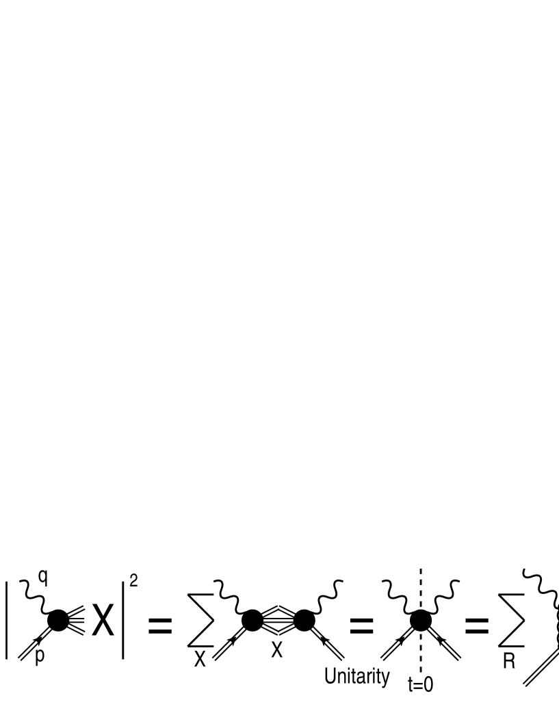
5mm normal

Figure 3: According to the Veneziano (or resonance-reggeon) duality a proper sum of either t-channel or s-channel resonance exchanges accounts for the whole amplitude. From JM1dama .

The kinematics of inclusive electron-nucleon scattering, applicable to both high energies, typical of HERA, and low energies as at JLab, is shown in Fig. 1. And Fig. 3 shows how DIS is related to the forward elastic (t=0) $\gamma^{*}p$ scattering, and then the latter is decomposed into a sum of the $s-$channel resonance exchanges.

The total cross section is related to the SF by

$$F_{2}(x,Q^{2})={Q^{2}(1-x)\over{4\pi\alpha(1+4m^{2}x^{2}/{Q^{2}})}}\sigma_{t}^{\gamma^{*}p}\leavevmode\nobreak\ ,$$ (31)

where $\alpha$ is the fine structure constant. In eq. (31) we neglected $R(x,Q^{2})=\sigma_{L}(x,Q^{2})/\sigma_{T}(x,Q^{2})$, which is a reasonable approximation.

The total cross section is related to the imaginary part of the scattering amplitude

$$\sigma_{t}^{\gamma^{*}p}(x,Q^{2})=\frac{8\pi}{P_{CM}\sqrt{s}}\,{\cal I}m\ A(s(x,Q^{2}),t=0,Q^{2})\leavevmode\nobreak\ .$$ (32)

where $P_{CM}$ is the center of mass momentum of the reaction,

$$P_{CM}=\frac{s-m^{2}}{2(1-x)}\sqrt{\frac{1+4m^{2}x^{2}/{Q^{2}}}{s}}$$ (33)

for DIS. Thus, we have

$$F_{2}(x,Q^{2})={4Q^{2}(1-x)^{2}\over{\alpha\left(s-m^{2}\right)(1+4m^{2}x^{2}/{Q^{2}})^{3/2}}}\,{\cal I}m\ A(s(x,Q^{2}),t=0,Q^{2})\,.$$ (34)

The minimal model for the scattering amplitude is a sum annalen

$$A(s,0,Q^{2})=c(s-u)(D(s,0,Q^{2})-D(u,0,Q^{2})),$$ (35)

providing the correct signature at high-energy limit, where $c$ is a normalization coefficient ($u$ is not an independent variable, since $s+u=2m^{2}-2Q^{2}$ or $u=-Q^{2}(1+x)/x+m^{2}$). As it was said at the beginning, we disregard the symmetry properties of the problem (spin and isospin), concentrating on its dynamics.

In the low $x$ limit: $x\rightarrow 0$, $t=0$, $Q^{2}=const$, $s=Q^{2}/x\rightarrow\infty$, $u=-s$, we obtain, with the help of eqs. (28,35):

$${\cal I}m\ A(s,0,Q^{2})|_{s\rightarrow\infty}\sim s^{\alpha_{t}(t)+\beta(0)+1}g^{\beta(Q^{2})}\,.$$ (36)

Our philosophy in this section is the following: we specify a particular choice of $\beta(Q^{2})$ in the low $x$ limit and then we use M-DAMA integral (3) to calculate the dual amplitude, and correspondingly SF, in all kinematical domains. We will see that the resulting SF has qualitatively correct behaviour in all regions. Even more - our choice of $\beta(Q^{2})$ will automatically remove $Q^{2}$ poles.

According to the two-component duality picture FH , both the scattering amplitude $A$ and the structure function $F_{2}$ are the sums of the diffractive and non-diffractive terms. At high energies both terms are of the Regge type. For $\gamma^{*}p$ scattering only the positive-signature exchanges are allowed. The dominant ones are the Pomeron and $f$ Reggeon, respectively. The relevant scattering amplitude is as follows:

$$B(s,Q^{2})=iR_{k}(Q^{2})\Bigl{(}{s\over{m^{2}}}\Bigr{)}^{\alpha_{k}(0)},$$ (37)

where $\alpha_{k}$ and $R_{k}$ are Regge trajectories and residues and $k$ stands either for the Pomeron or for the Reggeon. As usual, the residue is chosen to satisfy approximate Bjorken scaling for the SF BGP ; K . From eqs. (34,37) SF is given as:

$$F_{2}(x,Q^{2})\sim Q^{2}R_{k}(Q^{2})\Bigl{(}{s\over{m^{2}}}\Bigr{)}^{\alpha_{k}(0)-1}\,$$ (38)

where $x=Q^{2}/s$ in the limit $s\rightarrow\infty$.

It is obvious from eq. (38) that Regge asymptotics and scaling behaviour require the residue to fall like $\sim(Q^{2})^{-\alpha_{k}(0)}$. Actually, it could be more involved if we require the correct $Q^{2}\rightarrow 0$ limit to be respected and the observed scaling violation (the "HERA effect") to be included. Various models to cope with the above requirements have been suggested R8 ; BGP ; K . At HERA, especially at large $Q^{2}$, scaling is so badly violated that it may not be explicit anymore.

Data show that the Pomeron exchange leads to a rising structure function at large $s$ (low $x$). To provide for this we have two options: either to assume supercritical Pomeron with $\alpha_{P}(0)>1$ or to assume a critical ($\alpha_{P}(0)=1$) dipole (or higher multipole) Pomeron R8 ; wjs88 ; Pom1 . The latter leads to the logarithmic behaviour of the SF:

$$F_{2,P}(x,Q^{2})\sim Q^{2}R_{P}(Q^{2})\ln\Bigl{(}{s\over{m^{2}}}\Bigr{)}\,,$$ (39)

which proves to be equally efficient R8 ; Pom1 .

Let us now come back to M-DAMA results. Using eqs. (34,36) we obtain:

$$F_{2}\sim s^{\alpha_{t}(0)+\beta(0)}Q^{2}g^{\beta(Q^{2})}\,.$$ (40)

Choosing

$$\beta(0)=-1$$ (41)

we restore the asymptotics (38) and this allows us to use trajectories in their commonly used form. It is important to find such a $\beta(Q^{2})$, which can provide for Bjorken scaling (if one wants to take into account also the scaling violation then the problem just gets more technical). If we choose $\beta(Q^{2})$ in the form

$$\beta(Q^{2})=d-\gamma\ln(Q^{2}/Q_{0}^{2})\,,$$ (42)

with

$$\gamma=(\alpha_{t}(0)+\beta(0)+1)/\ln g=\alpha_{t}(0)/\ln g\,,$$ (43)

where $d$, $Q_{0}^{2}$ are some parameters, we get the exact Bjorken scaling.

Actually, the expression (42) might cause problems in the $Q^{2}\rightarrow 0$ limit. To avoid this, it is better to use a modified expressions

$$\beta(Q^{2})=\beta(0)-\gamma\ln\left(\frac{Q^{2}+Q_{0}^{2}}{Q_{0}^{2}}\right)=-1-\frac{\alpha_{t}(0)}{\ln g}\ln\left(\frac{Q^{2}+Q_{0}^{2}}{Q_{0}^{2}}\right)\,.$$ (44)

This choice leads to

$$F_{2}(x,Q^{2})\sim x^{1-\alpha_{t}(0)}\Bigl{(}{Q^{2}\over{Q^{2}+Q_{0}^{2}}}\Bigr{)}^{\alpha_{t}(0)}\,,$$ (45)

where the slowly varying factor $\Bigl{(}{Q^{2}\over{Q^{2}+Q_{0}^{2}}}\Bigr{)}^{\alpha_{t}(0)}$ is typical for the Bjorken scaling violation (see for example K ).

Now let us turn to the large $x$ limit. In this regime $x\rightarrow 1$, $s$ is fixed, $Q^{2}=\frac{s-m^{2}}{1-x}\rightarrow\infty$ and correspondingly $u=-2Q^{2}$. Using eqs. (30,34,35) we obtain:

$$F_{2}\sim(1-x)^{2}Q^{4}g^{2\beta(Q^{2}/2)}\sqrt{\frac{2\pi}{W^{\prime\prime}(z_{0})}}\left(g^{\alpha_{s}(s/2)}-g^{\alpha_{u}(-Q^{2})}\right)\,.$$ (46)

For $Q^{2}\rightarrow\infty$ factors $\left(g^{\alpha_{s}(s/2)}-g^{\alpha_{u}(-Q^{2})}\right)$ and $W^{\prime\prime}(z_{0})\approx 8\gamma\ln(Q^{2}/Q_{0}^{2})$ are slowly varying functions of $Q^{2}$ under our assumption about $\alpha_{u}(-Q^{2})$. Thus, we end up with

$$F_{2}\sim\left(\frac{2Q_{0}^{2}}{Q^{2}}\right)^{2\gamma\ln 2g}\sim(1-x)^{2\alpha_{t}(0)\ln 2g/\ln g}\,.$$ (47)

Let us now study $F_{2}$ given by M-DAMA in the resonance region. The existence of resonances in SF at large $x$ is not surprising by itself: as it follows from (32) and (34) they are the same as in $\gamma^{*}p$ total cross section, but in a different coordinate system.

For M-DAMA the resonances in $s$-channel are defined by the condition (7). For simplicity let us assume that we performed the Van der Corput neutralization and, thus, the pole terms appear in the form (19). In the vicinity of the resonance $s=s_{Res}$ only the resonance term $D_{Res}(s,0,Q^{2})$ is important in the scattering amplitude and correspondingly in the SF.

The complex pattern of the nucleon structure function in the resonance region was developed long time ago (see, for example Stein ). There are several dozens of resonances in the $\gamma^{*}p$ system in the region above pion-nucleon threshold, but only a few of them can be identified more or less unambiguously for various reasons. Therefore, instead of identifying each resonance, phenomenogists frequently considers a few maxima (usually 3) above the elastic scattering peak, corresponding to some ‘‘effective’’ resonance contributions. In the Regge-dual model JMfitnospin ; JMfitspin it was shown that for a reasonable fit it is enough to take into account three resonance terms, corresponding to "effective" $\Delta$, $N$, $N^{*}$ trajectories with one resonance on each, plus the background. As it was already discussed in the introduction, in the Regge-dual model the $Q^{2}$-dependence was introduced "by hands". Let us now check what we get from M-DAMA.

Using $\beta(Q^{2})$ in the form (44), which gives Bjorken scaling at large $s$, we obtain from eq. (16):

$$C_{1}(Q^{2})=\left(\frac{gQ_{0}^{2}}{Q^{2}+Q_{0}^{2}}\right)^{\alpha_{t}(0)}\left[\alpha_{t}(0)+\ln g\frac{Q^{2}}{Q^{2}+Q_{0}^{2}}-\frac{\alpha_{t}(0)}{\ln g}\ln\left(\frac{Q^{2}+Q_{0}^{2}}{Q_{0}^{2}}\right)\right]\,.$$ (48)

The term $\left(\frac{Q_{0}^{2}}{Q^{2}+Q_{0}^{2}}\right)^{\alpha_{t}(0)}$ gives the typical $Q^{2}$-dependence for the form factor (the rest is a slowly varying function of $Q^{2}$).

If we calculate higher orders of $C_{n}$ for subleading resonances, we will see that the $Q^{2}$-dependence is still defined by the same factor $\left(\frac{Q_{0}^{2}}{Q^{2}+Q_{0}^{2}}\right)^{\alpha_{t}(0)}$. Here comes the important difference from the Regge-dual model JMfitnospin ; JMfitspin motivated by introducing $Q^{2}$-dependence through the parameter $g$. As we see from eq. (19), $g$ enters with different powers for different resonances on one trajectory - the powers are increasing with the step 2. Thus, if $g\sim\left(\frac{Q_{0}^{2}}{Q^{2}+Q_{0}^{2}}\right)^{\bigtriangleup}$, then the form factor for the first resonance is ($n=0$) $\sim\left(\frac{Q_{0}^{2}}{Q^{2}+Q_{0}^{2}}\right)^{\bigtriangleup}$, and for the second one ($n=2$) it is $\sim\left(\frac{Q_{0}^{2}}{Q^{2}+Q_{0}^{2}}\right)^{3\bigtriangleup}$ etc. As discussed in JMfitspin the present accuracy of the data does not allow to discriminate between the constant powers of form factor (for example Refs. Stein ; Niculescu ; Osipenko ; DS , and this work) and increasing ones.

7 How to avoid $Q^{2}$ poles?

General study of the M-DAMA integral allows the $Q^{2}$ poles (see cases 2,4 in section 3), which would be unphysical. The appearance and properties of these singularities depend on the particular choice of the function $\beta(Q^{2})$, and for our choice, given by eq. (44), the $Q^{2}$ poles can be avoided.

We have chosen $\beta(Q^{2})$ to be a decreasing function, then, according to conditions (8,10), there are no $Q^{2}$ poles in M-DAMA in the physical domain $Q^{2}\geq 0$, if

$${\cal R}e\ \beta(0)<-\alpha_{s}(0)\,,\quad{\cal R}e\ \beta(0)<-\alpha_{t}(0)\,.$$ (49)

We have already fixed $\beta(0)=-1$, eq. (41), and, thus, we see that indeed we do not have $Q^{2}$ poles, except for the case of supercritical Pomeron with the intercept $\alpha_{P}(0)>1$. Such a supercritical Pomeron would generate one unphysical pole at $Q^{2}=Q^{2}_{pole}$ defined by equation

$$-1-{\alpha_{P}(0)\over\ln g}\ln\left(\frac{Q^{2}+Q_{0}^{2}}{Q_{0}^{2}}\right)+\alpha_{P}(0)=0\quad\Rightarrow\quad Q^{2}_{pole}=Q_{0}^{2}(g^{{\alpha_{P}(0)-1}\over\alpha_{P}(0)}-1)\,.$$ (50)

Therefore we can conclude that M-DAMA does not allow a supercritical trajectory - what is good from the theoretical point of view, since such a trajectory violates the Froissart-Martin limit Frois .

As it was discussed above there are other phenomenological models which use dipole Pomeron with the intercept $\alpha_{P}(0)=1$ and also fit the data (see for example R8 ). This is a very interesting case - ($\alpha_{t}(0)=1$) - for the proposed model. At the first glance it seems that we should anyway have a pole at $Q^{2}=0$. It should result from the collision of the moving pole $z=z_{0}$ with the branch point $z=0$, where $\alpha_{t}(0)+\beta(Q^{2}(1-z_{0}))=0$ in our case. Then, checking the conditions for such a collision:

$$\alpha_{t}(0)-t\,\alpha_{t}^{\prime}(0)z_{0}+\beta(Q^{2})-\beta^{\prime}(Q^{2})Q^{2}z_{0}=0\ \Rightarrow\ z_{0}=\frac{-\alpha_{t}(0)-\beta(Q^{2})}{t\,\alpha_{t}^{\prime}(0)-Q^{2}\beta^{\prime}(Q^{2})}\,,$$

we see that for $t=0$ and for $\beta(Q^{2})$ given by eq. (44) the collision is simply impossible, because $z_{0}(Q^{2})$ does not tend to $0$ for $Q^{2}\rightarrow 0$. Thus, for the Pomeron with $\alpha_{P}(0)=1$ M-DAMA does not contain any unphysical singularity.

On the other hand, a Pomeron trajectory with $\alpha_{P}(0)=1$ does not produce rising SF (38), as required by the experiment. So, we need a harder singularity and the simplest one is a dipole Pomeron. A dipole Pomeron produces poles of the second power:

$$D_{dipole}(s,t_{m})\propto\frac{C(s)}{(m-\alpha_{P}(t)+1)^{2}}\,,$$ (51)

usually the simple pole is also taken into account (we write a sum of simple pole and dipole) - see for example ref. wjs88 and references therein. Formally such a dipole Pomeron can be written as

$$\frac{\partial}{\partial\alpha_{P}}\frac{C(s)}{(m-\alpha_{P}(t)+1)}\,,$$

and generalizing this

$$D_{dipole}(s,t)=\frac{\partial}{\partial\alpha_{P}}D(s,t)\,,$$ (52)

where $D(s,t)$ can be given for example by DAMA or M-DAMA. Applying this expression to the asymptotic formula of M-DAMA, eq. (28), we obtain a term $g^{\beta(Q^{2})}s^{\alpha_{t}(t)+\beta(0)}\ln s$, which then leads to a logarithmically rising SF (for $\alpha_{P}(0)+\beta(0)=0$) - the one given by eq. (39).

For $\beta(Q^{2})$ in the form (44) M-DAMA will generate an infinite number of the $Q^{2}$ poles concentrated near the "ionization point" $Q^{2}=-Q^{2}_{0}$. Although these are in the unphysical region of negative $Q^{2}$, such a feature of the model
A) makes us think about $\beta(Q^{2})$ as about a kind of trajectory, what is not the case, as it was stressed above, and
B) might create a problem for a general theoretical treatment, for example for making analytical continuation in $Q^{2}$. To avoid this we can redefine $\beta(Q^{2})$ in the nonphysical $Q^{2}$ region, for example in the following way:

$$\beta(Q^{2})=\left\{\begin{array}[]{l}-1-\frac{\alpha_{t}(0)}{\ln g}\ln\left(\frac{Q^{2}+Q_{0}^{2}}{Q_{0}^{2}}\right)\,,\quad{\rm for}\ Q^{2}\geq 0\,,\\ -1-\frac{\alpha_{t}(0)}{\ln g}\ln\left(\frac{Q_{0}^{2}-Q^{2}}{Q_{0}^{2}}\right)\,,\quad{\rm for}\ Q^{2}<0\,.\end{array}\right.$$ (53)

This function has a maximum at $Q^{2}=0$, $\beta(0)=-1$. M-DAMA with $\beta(Q^{2})$ given by eq. (53) preserves all its good properties, discussed above, and does not contain any singularity in $Q^{2}$ (except for the supercritical Pomeron case, which we do not allow).

8 Conclusions

A new model for the $Q^{2}$-dependent dual amplitude with Mandelstam analyticity is proposed. The M-DAMA preserves all the attractive properties of DAMA, such as its pole structure and Regge asymptotics, but it also leads to generalized dual amplitude $A(s,t,Q^{2})$ and in this way realizes a unified "two-dimensionally dual" picture of strong interaction JM0dama ; JM1dama ; JMfitnospin ; JMfitspin (see Fig. 2). This amplitude, when $t=0$, can be related to the nuclear structure function. In section 6 we compare the SF generated by M-DAMA with phenomenological parameterizations, and in this way we fix the function $\beta(Q^{2})$, which introduces the $Q^{2}$-dependence in M-DAMA, eq. (3). The conclusion is that for both large and low $x$ limits as well as for the resonance region the results of M-DAMA are in qualitative agreement with the experiment.

General study of the M-DAMA integral tells us about the possibility to have poles in $Q^{2}$. These singularities may be avoided with our choice of $\beta(Q^{2})$, and also by putting restriction on the physical trajectories - the use of supercritical trajectory would lead to one $Q^{2}$ pole.

In the proposed formulation a $Q^{2}$-dependence is introduced into DAMA through the additional function $\beta(Q^{2})$. Although in the integrand this function stands next to Regge trajectories, this, as it was stressed already, does not mean that it also corresponds to some physical particles. There is no qualitative difference between two ways of introducing $Q^{2}$-dependence into DAMA: through the $Q^{2}$-dependent parameter $g$, i.e. function $g(Q^{2})$ JM0dama ; JM1dama or through the function $\beta(Q^{2})$. On the other hand the second way, i.e. M-DAMA, is applicable for all range of $Q^{2}$ and it results into physically correct behaviour in all tested limits.

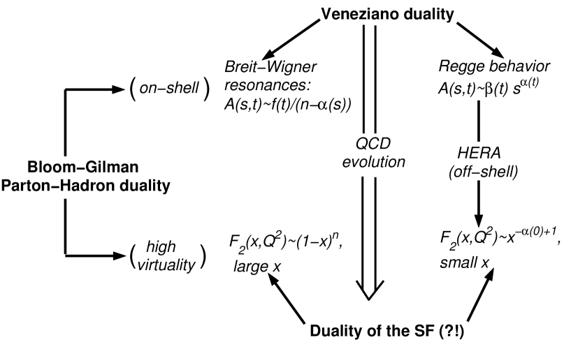
5mm normal

Figure 2: Veneziano, or resonance-reggeon duality Veneziano and Bloom-Gilman, or hadron-parton duality BG in strong interactions. From JM1dama .