HD-THEP-04-17

IFUM-789-FT

hep-ph/0404254

Towards a Nonperturbative Foundation
of the Dipole Picture:
I. Functional Methods

Carlo Ewerz ^a,b,1, Otto Nachtmann ^a,2

^a Institut für Theoretische Physik, Universität Heidelberg
Philosophenweg 16, D-69120 Heidelberg, Germany

^b Dipartimento di Fisica, Università di Milano and INFN, Sezione di Milano
Via Celoria 16, I-20133 Milano, Italy

This is the first of two papers in which we study real and virtual photon-proton scattering in a nonperturbative framework. We classify different contributions to this process and identify the leading contributions at high energies. We then study the renormalisation of the photon-quark-antiquark vertex that occurs in the leading contributions. We find something like the dipole picture in one of these contributions but also find two correction terms which can potentially become large at small photon virtualities. In the second paper we will discuss the additional approximations and assumptions that are necessary to obtain the dipole model of high energy scattering from the results found here.

  ¹ email: C.Ewerz@thphys.uni-heidelberg.de
² email: O.Nachtmann@thphys.uni-heidelberg.de

1 Introduction

The dipole picture of deep inelastic scattering at high energies [1]–[4] is a popular and successful way of describing and analysing the HERA data on electron-proton scattering, that is in particular quasi-real and virtual photon-proton scattering. In the recent past it has turned out that the framework of the dipole picture is well suited for studying the region of relatively small photon virtualities $Q^{2}$, that is the interesting transition region from perturbative to nonperturbative QCD. Particular interest concentrates on the problem of finding possible saturation effects occurring in that transition region. In essence, the dipole picture describes the deep inelastic photon-proton interaction as a two-step process in which the photon first splits into a quark-antiquark pair – a colour dipole – which then in the second step scatters off the proton. The first foundations on which the dipole picture rests were already laid in [5, 6]. For a general discussion of the dipole picture and for further references see [7]. One key problem in applying the dipole model in the transition region is to find a suitable description of the second step of the reaction, in other words to find the correct behaviour of the dipole-proton cross section. Models for this cross section have been developed and tested in inclusive as well as diffractive scattering processes, see for example [8]–[24]. Particularly popular is the Golec-Biernat–Wüsthoff model [8]–[10] which already in its first and simplest version gave a surprisingly good description of the HERA data. An important improvement of that model was obtained in [25] due to the inclusion of the correct logarithmic scaling violations according to DGLAP evolution at large $Q^{2}$ while preserving the success of the model at low $Q^{2}$. More recently, also the problem of describing the dependence of the dipole cross section on the impact parameter and hence the question of the $t$-distribution of the cross section has been addressed [26, 27].

The two-step nature of the scattering process described above is most easily visualised in a perturbative situation, and much of the theoretical development of the dipole model has been guided by the perturbative picture of deep inelastic scattering in QCD at high energies. Loosely speaking the dipole model tries to approach the transition to the nonperturbative region of small momenta from the perturbative side. Although its phenomenological success is rather encouraging it is not a priori clear that this method is in fact admissible. It is therefore very important to study whether there can be contributions to the cross section at low $Q^{2}$ which are not compatible with the formalism of the dipole model, that is contributions which cannot be correctly accommodated despite the freedom in modelling the low-$Q^{2}$ dipole-proton cross section. It is one aim of the present paper and the companion paper [28] (hereafter referred to as II) to address this question. One of our main results will in fact be the identification of two contributions to the amplitude which are not contained in the simple dipole picture. Both of these correction terms are small at large $Q^{2}$ but can become large at small $Q^{2}$. A second question which we consider to be important and which should be addressed in a nonperturbative framework is the following. It is frequently asserted that some sort of saturation must occur in real or virtual photon-proton scattering at high energies due to the Froissart-Martin-Lukaszuk bound on total cross sections. However, this bound applies only to hadron-hadron scattering and a priori is not valid for a current-induced reaction (see for instance [7]). It is usually argued that the dipole formula allows one to consider photon-proton scattering in essence as a hadron-proton reaction. But if one really wants to substantiate this type of reasoning and maybe some day derive an analogue of the Froissart-Martin-Lukaszuk bound for $\gamma p$ scattering one certainly should have a solid foundation for something like the dipole picture. It is our opinion that in order to achieve this goal one should not rely on perturbation theory alone.

In this work we start from a description of the real or virtual photon-proton scattering process in a generically nonperturbative framework developed by one of us in [29, 30]. This framework allows us to find a classification of different contributions to the cross section and to identify the approximations and assumptions that are necessary to arrive at the dipole model. We are able to identify two corrections to the dipole picture which can become large especially at low photon virtualities. In addition we find that our approach is also well suited to study two important problems which in our opinion have not yet been sufficiently appreciated so far. The first problem is that in QCD a mass-shell condition for quarks does not exist due to confinement. This is clearly not expected to be a serious problem in perturbative situations. However, if one wants to study high energy scattering in the nonperturbative domain this problem has to be taken very seriously. We will not be able to solve this deep problem in the present papers, but we hope to provide a framework in which at least the effects of assuming a mass-shell condition for quarks can be studied in more detail. The other important issue to which we would like to draw some attention concerns the electromagnetic gauge invariance in photon-proton scattering. It is well-known that gauge invariance in general imposes very strong restrictions on the amplitudes and on their factorisation. This has for example been discussed for the case of diffractive $\rho$ production at high energies in [31]. In II we find that important corrections to the simple dipole model are in fact required in order to ensure gauge invariance. It turns out that only at asymptotically high energies the simple dipole formula is obtained from the nonperturbative framework as a gauge invariant expression. This immediately raises the question whether presently accessible energies are large enough for the dipole picture to give a gauge invariant description in a sufficiently good approximation. Our framework should make it possible to address this important question in more detail.

The two papers are organised as follows. In the first paper we describe the general nonperturbative framework of our considerations and derive a classification of the contributions to the process of real or virtual Compton scattering on a proton. After discussing the relative importance of the different contributions we proceed to study in detail those which we expect to be leading in the high energy limit. In the further discussion we then focus on these contributions and discuss in particular the renormalisation of the photon-quark-antiquark vertex. The high energy limit of the amplitude obtained so far is then studied in the second paper. There we discuss how the usual formula for photon-proton scattering in the dipole picture emerges. Also in the second paper we discuss the important issue of gauge invariance. In particular we study how gauge invariance is manifest in the leading contribution to the scattering process. We then show that in the high energy limit different terms in the amplitude become gauge invariant separately. The perturbative wave function of the photon is derived and the consequences of gauge invariance for its correct definition are pointed out. Finally, we discuss some properties of the wave function of the photon and derive some simple phenomenological consequences of the dipole picture which can help to determine the limits of its applicability. We present our conclusions in II and point out some questions that in our opinion deserve further study. Some technical details of our calculations are presented in the appendices of the two papers.

2 Nonperturbative techniques and the dipole picture

Here we analyse photon induced reactions using nonperturbative techniques introduced in [29, 30]. The aim is to see if one can justify the dipole picture for high energies or if modifications of the dipole picture are necessary. Our method is quite general and can be applied to many processes.

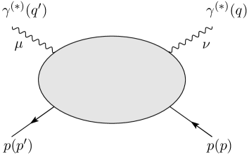
Figure 1: Compton scattering on a proton

For definiteness we consider real or virtual Compton scattering on a proton (see figure 1):

$$\gamma^{(*)}(q)+p(p)\,\,\,\longrightarrow\,\,\,\gamma^{(*)}(q^{\prime})+p(p^{\prime})\,,$$ (1)

where we indicate the four-momenta in brackets. For $q^{\prime}=q$ the absorptive part of the Compton amplitude can be related to spin-dependent and spin-independent structure functions. In the present papers we always work in leading order of the expansion in powers of the electromagnetic coupling $\alpha_{\rm em}$. Note that throughout this paper the figures are drawn such that the incoming particles are on the right hand side. We have chosen this ordering in order to make the correspondence of the figures with the equations as close as possible – despite the fact that the opposite choice is probably more common in the literature. We suppose

$$q^{2}=-Q^{2}\leq 0\,,\>\>\>\>\>q^{\prime\,2}=-Q^{\prime\,2}\leq 0\,,$$ (2)

but do not require $Q^{2}=Q^{\prime\,2}$. The usual Mandelstam variables are

$$s = (p+q)^{2}=(p^{\prime}+q^{\prime})^{2}\,,$$

$$t = (p-p^{\prime})^{2}=(q^{\prime}-q)^{2}\,,$$ (3)

$$u = (p-q^{\prime})^{2}=(p^{\prime}-q)^{2}\,.$$

Our procedure is rather general and allows us to treat the Compton amplitude for the case of real and virtual photons on the same footing. In the case of virtual photons our calculations apply to transversely as well as to longitudinally polarised photons. However, for the latter there are some subtleties in the high energy limit, as we will explain in II. We will at first keep to the cartesian indices $\mu,\nu=0,1,2,3$ for the photon polarisations.

Before going into the technical details let us now give a short non-technical description of our method. We use the reduction formula to represent the amplitude for our process (1) as an integral over vacuum expectation values of the currents and the fields for the protons. Then these vacuum expectation values are expressed as functional integrals in the usual way. Since the Lagrangian of QCD is bilinear in the quark degrees of freedom, $q$ and $\bar{q}$, we can perform the integrations over $q$ and $\bar{q}$. This allows us to give a classification of contributions to our amplitude in diagrammatic language according to the topology of the quark line skeleton, see figure 2 below. There the quark lines correspond to full quark propagators in a given external gluon field and the shaded blobs indicate the functional integration over all external gluon fields with a measure given below. The usual expectation is that at high energies the contribution shown in figure 2a will dominate. We show that also the diagram of figure 2b can give a leading contribution at high energies. We study first figure 2a in detail. We ‘cut’ the quark lines after the vertex where the photon $\gamma(q,\nu)$ enters the diagram and insert suitable factors 1, given by the Dirac operator times the free Green’s functions of the quarks. Integration by parts and the representation of the free Green’s functions of the quarks as dyadic products of quark and antiquark wave functions lead to four terms one of which can be interpreted as expected in the dipole picture. The photon $\gamma(q,\nu)$ splits into a quark-antiquark pair, which then interacts in all possible ways with the proton, see figures 7a and 8a below. However, these quarks and antiquarks are still off their energy shell, and one has to integrate over all these off-shell energies. But at high energies the leading contribution comes from the on-shell quarks. This corresponds to the contribution of a certain pinch singularity in the amplitudes considered as functions in the (off-shell) energy plane. Adding now the contribution of the diagram of figure 2b, treated in a similar way, we have indeed described the original amplitude for the process (1) at high energies as a two step process. The leading term of the amplitude is given as a convolution of the bare $\gamma q\bar{q}$ vertex function with a scattering amplitude for a bare $q\bar{q}$ pair on the proton. It remains to introduce the renormalised quantities in place of the bare ones. This we do by using the Dyson-Schwinger equation for the $\gamma q\bar{q}$ vertex function which contains all higher order QCD corrections to the vertex. Here our approach is inspired by the standard treatment of overlapping divergences in QED. Finally, we arrive at the expression shown graphically in figures 10 and 11 below. The leading contribution to the amplitude for the reaction (1) at high energies is given by two terms. The first one is a convolution of the renormalised $\gamma q\bar{q}$ vertex function, describing the splitting of the photon to the $q\bar{q}$ pair, with the renormalised amplitude for $q\bar{q}+p\rightarrow\gamma(q^{\prime},\mu)+p$. The second term describes rescattering corrections. Thus, on the side of the colour dipole amplitude, the contribution ${\cal T}^{(b)}$ from the diagram of figure 2b must be added, and on the side of the incoming photon, we find the rescattering correction. These additional terms are also leading at high energies and could be important for phenomenology especially at small photon virtualities.

In addition to deriving this general structure of the amplitude for (1) at high energies we discuss in II the problem of electromagnetic gauge invariance and the related subtleties for the amplitudes of longitudinally polarised virtual photons. In summary, from the contribution of figure 2a and 2b we find something like the dipole picture at high energies. But usually only the term ${\cal T}^{(a)}$ from the diagram of figure 2a times the photon vertex function is discussed in the dipole model. We find important additional terms as mentioned above.

A key step in our procedure is to cut the amplitude next to the vertex of the incoming photon and to insert a factor 1 consisting of the Dirac operator and of Green’s functions of the quarks. A similar step has of course been used more or less explicitly in many studies of the Compton amplitude or of diffractive photon-proton scattering. Many of those investigations are, however, restricted to the case of virtual photons in which perturbation theory can be applied. In our method this step is used in the framework of a nonperturbative description of the real and the virtual Compton amplitude. But several technical aspects of our method clearly resemble those studies, see for example [32, 33] and also [34, 35].

After this outline of our procedure we now turn to the actual calculations. These involve sometimes lengthy formulae. But we hope that the figures accompanying them will, nevertheless, make them transparent. We should point out again that in order to make the correspondence between the equations and the figures as easy as possible all figures are drawn such that they are to be read from right to left.

2.1 Classification of contributions to real or virtual Compton scattering

The matrix element for the reaction (1) is

$$\mathcal{M}^{\mu\nu}_{s^{\prime}s}(p^{\prime},p,q)=\frac{i}{2\pi m_{p}}\int d^{4}x~{}e^{-iqx}\langle p(p^{\prime},s^{\prime})|\mbox{T}^{*}J^{\mu}(0)J^{\nu}(x)|p(p,s)\rangle\,,$$ (4)

where $m_{p}$ is the proton mass, $s,s^{\prime}=\pm 1/2$ are the spin indices, and $\mbox{T}^{*}$ is the covariantised T-product. Our proton states are normalised to

$$\langle p(p^{\prime},s^{\prime})|p(p,s)\rangle=2p^{0}(2\pi)^{3}\delta_{s^{\prime}s}\,\delta^{(3)}(\mathbf{p}^{\prime}-\mathbf{p})\,.$$ (5)

All our conventions regarding kinematics, Dirac spinors etc. follow [36].

The hadronic part of the electromagnetic current is denoted by

$$J^{\lambda}(x)=\sum_{q}\bar{q}(x)Q_{q}\gamma^{\lambda}q(x)\,,$$ (6)

where $q=u,d,\dots$ are the quark field operators and $Q_{u}=2/3,Q_{d}=-1/3,\dots$ are the quark charges in units of the proton charge.

Let $\psi_{p}(x)$ be a suitable interpolating field operator for the proton. We can take $\psi_{p}$ to contain three quark fields,

$$\psi_{p}(x)=\Gamma_{\alpha\beta\gamma}u_{\alpha}(x)u_{\beta}(x)d_{\gamma}(x)\,,$$ (7)

and accordingly

$$\bar{\psi}_{p}(x)=\bar{\Gamma}_{\alpha\beta\gamma}\bar{d}_{\gamma}(x)\bar{u}_{\beta}(x)\bar{u}_{\alpha}(x)\,,$$ (8)

where $\Gamma_{\alpha\beta\gamma}$ and $\bar{\Gamma}_{\alpha\beta\gamma}$ are coefficient matrices and $\alpha,\beta,\gamma$ summarize Dirac and colour indices. Explicit constructions of field operators $\psi_{p}(x)$ of the type (7) can be found in [37, 38, 39]. Let $Z_{p}$ be the proton’s wave function renormalisation constant defined by

$$\left\langle 0|\psi_{p}(x)|p(p,s)\right\rangle=\sqrt{Z_{p}}\,e^{-ipx}u_{s}(p)\,.$$ (9)

Using now the LSZ reduction formula [40] and the representation of Green’s functions by the functional integral we get

$$\mathcal{M}^{\mu\nu}_{s^{\prime}s}(p^{\prime},p,q) = -\frac{i}{2\pi m_{p}Z_{p}}\int d^{4}y^{\prime}~{}d^{4}y~{}d^{4}x\,e^{ip^{\prime}y^{\prime}}\bar{u}_{s^{\prime}}(p^{\prime})(-i\!\stackrel{{\scriptstyle\rightarrow}}{{\!\not\!\partial}}_{y^{\prime}}+m_{p})$$

$${}\left\langle\psi_{p}(y^{\prime})J^{\mu}(0)e^{-iqx}J^{\nu}(x)\overline{\psi}_{p}(y)\right\rangle_{G,q,\bar{q}}\,(i\!\stackrel{{\scriptstyle\leftarrow}}{{\!\not\!\partial}}_{y}+m_{p})u_{s}(p)e^{-ipy}\,.$$

Here we use a shorthand notation for the functional integral. For any functional $F(G,q,\bar{q})$ of gluon and quark fields we write

$$\left\langle F(G,q,\bar{q})\right\rangle_{G,q,\bar{q}}=\frac{1}{\mathcal{Z}}\int\mathcal{D}(G,q,\bar{q})F(G,q,\bar{q})\exp\left[i\int d^{4}x\,{\cal L}_{\mbox{\scriptsize QCD}}(x)\right]\,,$$ (11)

with

$$\mathcal{Z}=\int\mathcal{D}(G,q,\bar{q})\exp\left[i\int d^{4}x\,{\cal L}_{\mbox{\scriptsize QCD}}(x)\right]\,.$$ (12)

Of course, on the r.h.s. of (2.1), the quark-field operators in $J^{\mu}$ and $\psi_{p}$ are to be replaced by the corresponding Grassmann integration variables of the functional integral. Gauge fixing and Faddeev-Popov terms in the functional integral are implied and not written out explicitly.

In (2.1) we have used translational invariance to shift the argument of the current $J^{\mu}$ to zero. In the following this makes our procedure look somewhat asymmetric with respect to the treatment of the two currents $J^{\mu}$ and $J^{\nu}$. We could equally well make the treatment completely symmetric with respect to $J^{\mu}$ and $J^{\nu}$ by shifting the argument of $\psi_{p}$ or $\bar{\psi}_{p}$ to zero in (2.1), see appendix A.

Since the Lagrangian of QCD is bilinear in the quark fields, we can immediately perform the $q,\bar{q}$ functional integral. This leads to a number of terms representing all possible contractions of quark and antiquark field operators, as is explained in appendix A. The resulting terms can be classified in terms of the quark line skeleton in the graphical representation of the amplitude. The different types of contributions to the amplitude are shown pictorially in figure 2, the explicit formulae for all terms are given explicitly in appendix A.

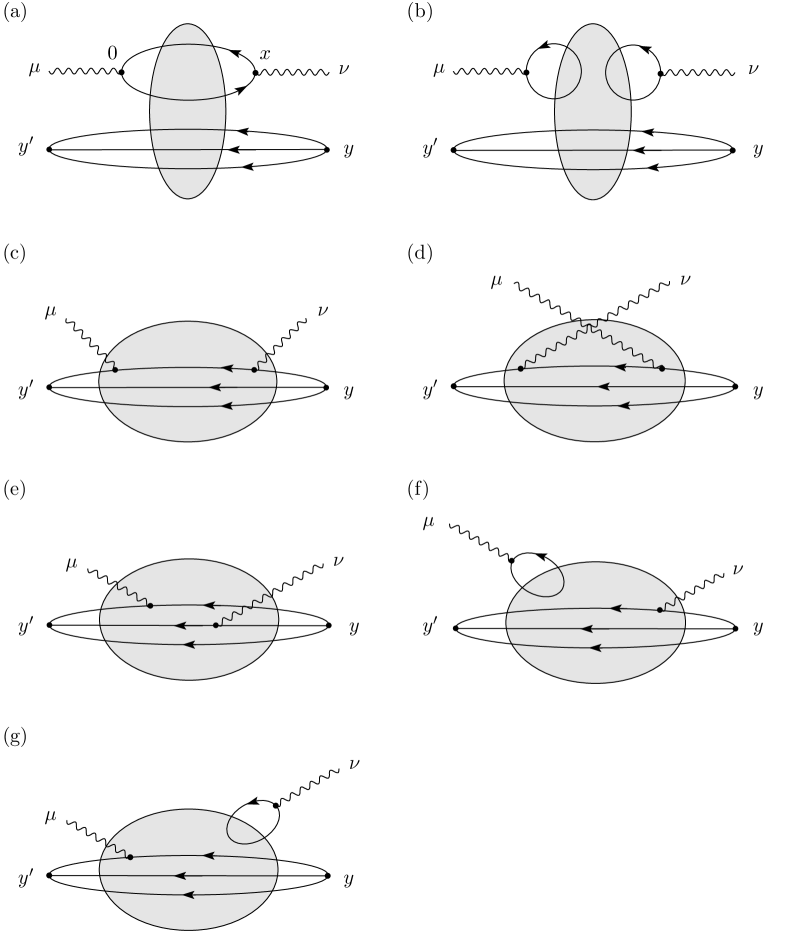
Figure 2: The diagrams resulting from the functional integral (A.8) corresponding to ${\cal J}^{(a)},\dots,{\cal J}^{(g)}$ and to the amplitudes ${\cal M}^{(a)},\dots,{\cal M}^{(g)}$ of (13)

In figure 2 each quark line corresponds to a full quark propagator in a given external gluon potential. An integration over all gluon potentials with a functional integral measure including the fermion determinant is implied. Corresponding to the diagrams of figure 2 we get the following decomposition of $\mathcal{M}^{\mu\nu}_{s^{\prime}s}$ (2.1):

$$\mathcal{M}^{\mu\nu}_{s^{\prime}s}(p^{\prime},p,q)=\mathcal{M}^{(a)\mu\nu}_{s^{\prime}s}(p^{\prime},p,q)+\ldots+\mathcal{M}^{(g)\mu\nu}_{s^{\prime}s}(p^{\prime},p,q)\,.$$ (13)

Putting all factors together we get for instance for $\mathcal{M}^{(a)\mu\nu}_{s^{\prime}s}$ (see figure 2a)

$$\mathcal{M}^{(a)\mu\nu}_{s^{\prime}s}(p^{\prime},p,q) = -\frac{i}{2\pi m_{p}Z_{p}}\int d^{4}y^{\prime}~{}d^{4}y\,e^{ip^{\prime}y^{\prime}}\bar{u}_{s^{\prime}}(p^{\prime})(-i\!\stackrel{{\scriptstyle\rightarrow}}{{\!\not\!\partial}}_{y^{\prime}}+m_{p})$$ (17)

$${}\sum_{q}Q^{2}_{q}\Big{\langle}\mathop{\vbox{\halign{#\cr\kern 1.72218pt\cr$\hbox{$\hskip 3.25696pt\vrule height=7.31946pt,width=0.29999pt,depth=-0.11153pt\kern-0.29999pt\vrule height=7.31946pt,width=23.15385pt,depth=-7.01947pt\kern-0.29999pt\vrule height=7.31946pt,width=0.29999pt,depth=1.15515pt$\hss}$\crcr\kern 1.72218pt\nointerlineskip\cr\hbox{$\displaystyle{}{\psi}{{}_{p}(y^{\prime})}{\overline{\psi}}_{p}(y)$}\crcr}}}\limits A^{(q)\mu\nu}(q)\Big{\rangle}_{G}\,(i\!\stackrel{{\scriptstyle\leftarrow}}{{\!\not\!\partial}}_{y}+m_{p})u_{s}(p)e^{-ipy}\,,$$

where the contraction $\mathop{\vbox{\halign{#\cr\kern 1.72218pt\cr$\hbox{$\hskip 3.25696pt\vrule height=7.31946pt,width=0.29999pt,depth=-0.11153pt\kern-0.29999pt\vrule height=7.31946pt,width=23.15385pt,depth=-7.01947pt\kern-0.29999pt\vrule height=7.31946pt,width=0.29999pt,depth=1.15515pt$\hss}$\crcr\kern 1.72218pt\nointerlineskip\cr\hbox{$\displaystyle{}{\psi}{{}_{p}(y^{\prime})}{\overline{\psi}}_{p}(y)$}\crcr}}}\limits$ is defined in (A.14) and

$$A^{(q)\mu\nu}(q)=\int d^{4}x\,\mathrm{Tr}\left[\gamma^{\mu}S^{(q)}_{F}(0,x;G)e^{-iqx}\gamma^{\nu}S^{(q)}_{F}(x,0;G)\right]\,.$$ (18)

Here $S^{(q)}_{F}(x,y;G)$ is the propagator for quark flavor $q$ in the external gluon potential $G$,

$$(i\gamma^{\mu}D_{\mu}-m^{(0)}_{q})S^{(q)}_{F}(x,y;G)=-\delta^{(4)}(x-y)\,.$$ (19)

In (17) we denote by $\langle\cdot\rangle_{G}$ the functional integral over the gluonic degrees of freedom, including the fermion determinant. That is, we define for any functional $F[G]$

$$\left\langle F[G]\right\rangle_{G} = \frac{1}{\mathcal{Z}^{\prime}}\int\mathcal{D}(G)F[G]\,\prod\limits_{q}\det\left[-i(i\gamma^{\lambda}D_{\lambda}-m^{(0)}_{q}+i\epsilon)\right]$$ (20)

$${}\exp\left[-i\int d^{4}x\,\frac{1}{2}\mathrm{Tr}\left(G_{\lambda\rho}(x)G^{\lambda\rho}(x)\right)\right]\,,$$

where $\mathcal{Z}^{\prime}$ is the normalisation factor obtained from the condition

$$\langle 1\rangle_{G}=1\,.$$ (21)

Again gauge fixing and Faddeev-Popov terms are implied.

In a similar way we get from (A.9) and (A.15) for the amplitude $\mathcal{M}^{(b)\mu\nu}_{s^{\prime}s}$ corresponding to figure 2b

$$\mathcal{M}^{(b)\mu\nu}_{s^{\prime}s}(p^{\prime},p,q) = -\frac{i}{2\pi m_{p}Z_{p}}\int d^{4}y^{\prime}~{}d^{4}y\,e^{ip^{\prime}y^{\prime}}\bar{u}_{s^{\prime}}(p^{\prime})(-i\!\stackrel{{\scriptstyle\rightarrow}}{{\!\not\!\partial}}_{y^{\prime}}+m_{p})$$

$${}\sum_{q^{\prime},q}Q_{q^{\prime}}Q_{q}\Big{\langle}\mathop{\vbox{\halign{#\cr\kern 1.72218pt\cr$\hbox{$\hskip 3.25696pt\vrule height=7.31946pt,width=0.29999pt,depth=-0.11153pt\kern-0.29999pt\vrule height=7.31946pt,width=23.15385pt,depth=-7.01947pt\kern-0.29999pt\vrule height=7.31946pt,width=0.29999pt,depth=1.15515pt$\hss}$\crcr\kern 1.72218pt\nointerlineskip\cr\hbox{$\displaystyle{}{\psi}{{}_{p}(y^{\prime})}{\overline{\psi}}_{p}(y)$}\crcr}}}\limits(-1)\mathrm{Tr}\left[\gamma^{\mu}S_{F}^{(q^{\prime})}(0,0;G)\right]$$

$${}\int d^{4}x\,\mathrm{Tr}\left[e^{-iqx}\gamma^{\nu}S_{F}^{(q)}(x,x;G)\right]\Big{\rangle}_{G}(i\!\stackrel{{\scriptstyle\leftarrow}}{{\!\not\!\partial}}_{y}+m_{p})u_{s}(p)e^{-ipy}\,.$$

The corresponding expressions for the other contributions $\mathcal{M}^{(c)}$ - $\mathcal{M}^{(g)}$ are given explicitly in appendix A.

The methods used here for the classification of different contributions to the amplitude can also be applied to other current induced reactions at high energies. In the case of exclusive reactions for example one chooses appropriate interpolating field operators for the produced hadrons and can proceed exactly as discussed here for the Compton amplitude.

2.2 Relative size of different contributions

With the diagrams of figure 2 we have given a classification of all contributions to the Compton amplitude, see (13). At high energies $\sqrt{s}$ we expect the diagrams of figures 2a and 2b, that is $\mathcal{M}^{(a)}$ of (17) and $\mathcal{M}^{(b)}$ of (2.1), to give the dominant contribution. Indeed, let us consider the diagrams of figures 2a-2g for large $\sqrt{s}$. In figure 2c for instance we find at Born level that a large momentum of order $\sqrt{s}$ has to flow through the upper quark line. This leads to a suppression of order $1/\sqrt{s}$ relative to the diagrams of figures 2a, 2b. Similar arguments apply to the diagrams of figures 2d-2g.

Going one step further in sophistication we can have a look at resummed perturbation theory. In the perturbative framework the generic diagrams of figures 2a and 2b include gluon ladder diagrams, see figures 3 and 4, respectively.

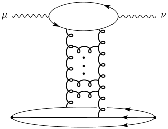
Figure 3: Perturbative gluon ladder diagram which is contained in the generic diagram of figure 2a for the amplitude $\mathcal{M}^{(a)}$

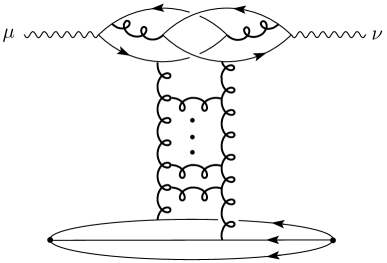
Figure 4: Perturbative gluon ladder diagram which is contained in the generic diagram of figure 2b for the amplitude $\mathcal{M}^{(b)}$

These are, of course, just the diagrams containing the leading order BFKL pomeron exchange [41, 42]. The leading perturbative diagrams contained in the generic diagrams of figures 2c-2g, on the other hand, do not contain such gluon ladders. Instead, they typically contain quark-antiquark exchanges in the $t$-channel. As an example figure 5 shows a perturbative quark ladder diagram contributing to the generic diagram of figure 2c.

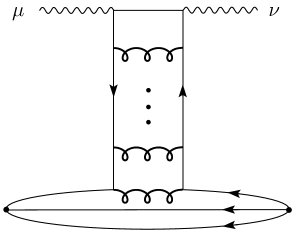
Figure 5: Perturbative quark ladder diagram which is contained in the generic diagram of figure 2c for the amplitude $\mathcal{M}^{(c)}$

But it is well known that diagrams with quark-antiquark exchanges (or more generally fermion-antifermion exchanges) in the $t$-channel are suppressed by powers of the energy with respect to the corresponding diagrams containing gluon (or more generally vector boson) exchanges. Similarly, also the generic diagrams in figures 2d and 2e contain quark-antiquark exchanges as the leading terms in perturbation theory. Presumably also the leading terms of the generic diagrams of figures 2f and 2g correspond to quark-antiquark exchanges, see figure 6,

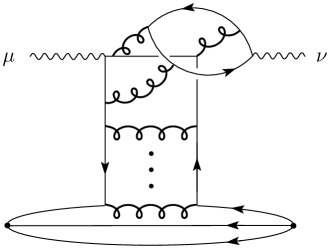
Figure 6: Perturbative diagram which is contained in the generic diagram of figure 2g for the amplitude $\mathcal{M}^{(g)}$

where this is shown for the diagram of figure 2g. We can hence conclude that the leading perturbative diagrams for the generic diagrams of figures 2c-2g are suppressed by powers of $\sqrt{s}$ with respect to the leading perturbative contributions to the amplitudes $\mathcal{M}^{(a)}$ and $\mathcal{M}^{(b)}$.

We also arrive at the same conclusion when we switch from perturbation theory to Regge theory. Quite generally, we expect the dominant contribution from the diagrams of figures 2a and 2b to be due to pomeron exchange, soft and hard, with its well-known phenomenological properties, see for instance [7]. On the other hand, we estimate that the main contribution from the generic diagram of figure 2c for large $\sqrt{s}$ is due to reggeon exchange which would correspond to the diagram of figure 5, now interpreted as a diagram of Regge theory. Again, we know from phenomenology that reggeon exchanges are suppressed by a factor of roughly $1/\sqrt{s}$ relative to soft pomeron exchange, see [7]. Thus we can argue that the generic diagrams of figure 2c and in a similar way those of figures 2d and 2e correspond to reggeon exchanges and are thus not leading for large $\sqrt{s}$. The same holds for the diagrams of figures 2f and 2g, as is illustrated in figure 6. Again we find that the amplitudes $\mathcal{M}^{(c)}$ - $\mathcal{M}^{(g)}$ are subleading at high energy $\sqrt{s}$.

Let us now discuss the relative magnitudes of the amplitudes $\mathcal{M}^{(a)}$ and $\mathcal{M}^{(b)}$ corresponding to the figures 3 and 4. At high energies the leading contributions to both amplitudes have the same dependence on the energy. As discussed above that dependence results from Pomeron exchange or from gluon ladder diagrams, depending on whether one describes it in terms of Regge theory or perturbative QCD (pQCD). The typical perturbative diagrams are shown in figures 3 and 4, respectively, and in pQCD these diagrams represent the leading contribution at high energies. The main difference between the two amplitudes is the coupling of the gluon ladder (or the Pomeron) to the incoming and outgoing photon, or in perturbative language the impact factor. In the impact factor in $\mathcal{M}^{(b)}$ there are two quark loops which are connected by gluon lines. Due to the charge parity of the photon a minimum number of three gluons is required to couple to each of these loops, and the diagram shown in figure 4 is hence the lowest order contribution to the impact factor of $\mathcal{M}^{(b)}$. Compared with the amplitude $\mathcal{M}^{(a)}$ the amplitude $\mathcal{M}^{(b)}$ therefore contains two additional factors of $\alpha_{s}$ which are not compensated by any large logarithms. The relevant scale of $\alpha_{s}$ is determined by the photon virtuality $Q^{2}$. Consequently, the amplitude $\mathcal{M}^{(b)}$ is strongly suppressed at high virtualities. At small virtualities, however, $\alpha_{s}$ becomes large and that suppression is no longer relevant. Besides these factors of $\alpha_{s}$ there appears to be no other simple mechanism suppressing the diagrams of figure 4. Accordingly, these diagrams can potentially give an important contribution in the region of low photon virtualities. In our opinion their contribution, which is often neglected in applications of the dipole picture of high energy scattering, deserves further study. It would be especially interesting to find ways of estimating the relative size of the terms $\mathcal{M}^{(a)}$ and $\mathcal{M}^{(b)}$ at low $Q^{2}$ using experimental data.

It should be noted here that in our development of the dipole picture below we find that perturbative diagrams contained in figures 2a and 2b contribute to the colour dipole amplitude side and photon wave function side such that one can speak of a mixing of the diagram classes (a) and (b) in the colour dipole picture. This is relevant in higher orders in $\alpha_{s}$ as we will discuss when we make the transition to renormalised quantities in section 2.4 below. The preceding discussion refers to the leading terms (at large $\sqrt{s}$ and large $Q^{2}$) and is therefore not affected by this effect.

From the observations made here we conclude that at high energies the amplitude $\mathcal{M}^{(a)}$ is expected to give the leading contribution if the photon virtuality is large, and that at lower virtualities also the amplitude $\mathcal{M}^{(b)}$ should become important. We will therefore in the following discuss in detail the amplitude $\mathcal{M}^{(a)}$, given in (17), which corresponds to the diagram of figure 2a. For the amplitude $\mathcal{M}^{(b)}$, figure 2b, the same steps can be done in a completely analogous way, see appendix C.

Finally we note that for the hypothetical case of scattering of an isovector photon on an $\Omega^{-}$ target only the diagram of figure 2a exists as long as one assumes equal up and down quark masses and neglects higher orders in the electromagnetic coupling $\alpha_{\rm em}$, as we do throughout the present papers. Indeed, in this case the current has the structure

$$J^{\mu}_{\rm isovector}=\frac{1}{2}\bar{u}\gamma^{\mu}u-\frac{1}{2}\bar{d}\gamma^{\mu}d\,,$$ (26)

whereas the $\Omega^{-}$ consists of three $s$-quarks. Thus none of the diagrams of figures 2b-2g can be drawn for this case and $\mathcal{M}^{(a)}$ gives the complete amplitude.

2.3 From current to quark scattering for a fixed gluon potential

In the following we consider the diagram of figure 2a. We will in essence cut the quark lines at the vertex marked $x$, insert factors of $1$, and relate the amplitude for the scattering of the photon on the proton to that of scattering of a $q\bar{q}$ pair on the proton. We recall first that the free quark propagator for mass $m_{q}$ satisfies

$$(i\!\stackrel{{\scriptstyle\rightarrow}}{{\!\not\!\partial}}_{x}-m_{q})S_{F}^{(q,0)}(x,y) = {}-\delta^{(4)}(x-y)\,,$$ (27)

$$S^{(q,0)}_{F}(x,y)(i\!\stackrel{{\scriptstyle\leftarrow}}{{\!\not\!\partial}}_{y}+m_{q}) = {}\delta^{(4)}(x-y)\,.$$ (28)

A simple exercise shows that $S_{F}^{(q,0)}$ can be written as a sum of dyadic products of quark and antiquark wave functions, see (B.15) of appendix B.

We shall now use (27), (28) and (B.15) to rewrite $A^{(q)\mu\nu}(q)$ of (18) in a form where we can make the transition from current scattering to $q\bar{q}$ scattering. Inserting factors of one in (18) we get

$$A^{(q)\mu\nu}(q) = \int d^{4}x~{}d^{4}z~{}d^{4}z^{\prime}\,\mathrm{Tr}\left[\gamma^{\mu}S^{(q)}_{F}(0,z;G)\delta^{(4)}(z-x)\right.$$ (29)

$${}\left.e^{-iqx}\gamma^{\nu}\delta^{(4)}(x-z^{\prime})S^{(q)}_{F}(z^{\prime},0;G)\right]$$

$$= \int d^{4}x~{}d^{4}z~{}d^{4}z^{\prime}\,\mathrm{Tr}\left[\gamma^{\mu}S^{(q)}_{F}(0,z;G)(-i\!\stackrel{{\scriptstyle\rightarrow}}{{\!\not\!\partial}}_{z}+m_{q})S^{(q,0)}_{F}(z,x)\right.$$

$${}\left.e^{-iqx}\gamma^{\nu}S^{(q,0)}_{F}(x,z^{\prime})(i\!\stackrel{{\scriptstyle\leftarrow}}{{\!\not\!\partial}}_{z^{\prime}}+m_{q})S^{(q)}_{F}(z^{\prime},0;G)\right]\,.$$

Integration by parts and use of (B.15) leads us to a representation of $A^{(q)\mu\nu}(q)$ as a sum of four terms which we can interpret in terms of $q$ and $\bar{q}$ scattering. The key step in using (B.15) is a decomposition of the free propagator $S^{(q,0)}_{F}$ as a spin and colour sum over Dirac spinors, see (B.4), (B.5). Those spinors immediately lead to an interpretation in terms of quarks and antiquarks. The details are given in appendix B. The final result derived there is (see (B))

$$A^{(q)\mu\nu}(q)=\sum^{4}_{j=1}A^{(q)\mu\nu}_{j}(q)\,,$$ (30)

where

$$A^{(q)\mu\nu}_{j}(q)=\frac{1}{2\pi}\int\frac{d\omega}{\omega+i\epsilon}\int\frac{d^{3}k}{(2\pi)^{3}2k^{0}}\,a_{j}\,,$$ (31)

with

$$a_{1} = -\sum_{r,r^{\prime}}(\overline{k^{\prime(1)}_{\omega},r^{\prime}}|B^{(q)\mu}|k_{\omega},r)\bar{u}_{r}(k)\gamma^{\nu}v_{r^{\prime}}(k^{{\prime}(1)})$$ (32)

$${}(q^{0}-k^{0}-k^{\prime(1)0}-\omega+i\epsilon)^{-1}(2k^{\prime(1)0})^{-1}\,,$$

$$a_{2} = \sum_{r,r^{\prime}}(k^{\prime(2)}_{\omega},r^{\prime}|B^{(q)\mu}|k_{\omega},r)\bar{u}_{r}(k)\gamma^{\nu}u_{r^{\prime}}(k^{{\prime}(2)})$$ (33)

$${}(-q^{0}+k^{0}-k^{\prime(2)0}+\omega+i\epsilon)^{-1}(2k^{\prime(2)0})^{-1}\,,$$

$$a_{3} = -\sum_{r,r^{\prime}}(k^{\prime(3)}_{\omega},r^{\prime}|B^{(q)\mu}|\overline{k_{\omega},r})\bar{v}_{r}(k)\gamma^{\nu}u_{r^{\prime}}(k^{{\prime}(3)})$$ (34)

$${}(-q^{0}-k^{0}-k^{\prime(3)0}-\omega+i\epsilon)^{-1}(2k^{\prime(3)0})^{-1}\,,$$

$$a_{4} = \sum_{r,r^{\prime}}(\overline{k^{\prime(4)}_{\omega},r^{\prime}}|B^{(q)\mu}|\overline{k_{\omega},r})\bar{v}_{r}(k)\gamma^{\nu}v_{r^{\prime}}(k^{{\prime}(4)})$$ (35)

$${}(q^{0}+k^{0}-k^{\prime(4)0}+\omega+i\epsilon)^{-1}(2k^{\prime(4)0})^{-1}\,.$$

The operator $B^{(q)\mu}$ is defined in (B.24) and $k^{\prime(j)},k^{\prime(j)}_{\omega}$ in (B)-(B). Here $r,r^{\prime}$ are spin and colour indices with $r=(\lambda,A)$, $\lambda=\pm 1/2$ and $A=1,2,3$. The four terms are illustrated in figure 7.

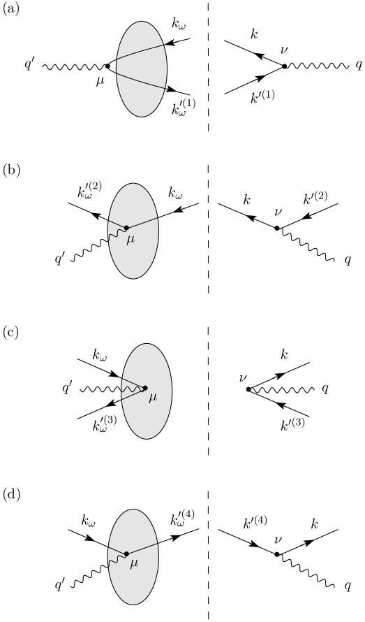
Figure 7: Interpretation of the four terms $A_{j}^{(q)\mu\nu}(q)$ of (31) where $j=1,\dots,4$ corresponds to (a), …, (d). The shading indicates the fixed gluon potential. The arrows on the lines indicate the interpretation as quark or antiquark. The orientation of the momentum assignment to the lines is from right to left for all lines, irrespective of the arrows on the lines.

In that figure the dashed vertical line indicates an integration over $\omega$ and over the three-momentum $\mathbf{k}$ according to (31). We emphasise that the vertical line does not imply that all quark and antiquark lines are set on-shell, see the discussion below. The arrows on the lines indicate the interpretation as quark or antiquark. The orientation of the momentum assignment to the lines is from right to left for all lines, irrespective of the arrows on the lines. The interpretation of $A^{(q)\mu\nu}_{j}(q)$ is now easily obtained (see figure 7):

• The term $A^{(q)\mu\nu}_{1}(q)$ corresponds in essence to the splitting of the initial real or virtual photon into a $q\bar{q}$ pair with momenta $k,k^{\prime(1)}$. This is combined with the amplitude for a $q\bar{q}$ pair of momenta $k_{\omega},k^{\prime(1)}_{\omega}$ scattering on the fixed gluon potential and recombining to the final real or virtual photon $q^{\prime}$ (figure 7a).

• The term $A^{(q)\mu\nu}_{2}(q)$ corresponds to a quark of momentum $k^{\prime(2)}$ absorbing the photon $q$ and going to a quark of momentum $k$. This is combined with the amplitude for a quark $k_{\omega}$ shaking off a photon $q^{\prime}$ in the fixed gluon potential and going to quark $k^{\prime(2)}_{\omega}$ (figure 7b).

• The term $A^{(q)\mu\nu}_{3}(q)$ corresponds to an antiquark $k$ and quark $k^{\prime(3)}$ annihilating by absorption of a photon $q$. This is combined with the amplitude for the creation of a quark $k^{\prime(3)}_{\omega}$, antiquark $k_{\omega}$ and photon $q^{\prime}$ in the fixed gluon potential (figure 7c).

• The term $A^{(q)\mu\nu}_{4}(q)$ corresponds to an antiquark $k$ absorbing a photon $q$ and going to an antiquark $k^{\prime(4)}$. This is combined with the amplitude for an antiquark $k^{\prime(4)}_{\omega}$ going to an antiquark $k_{\omega}$ with emission of a photon $q^{\prime}$ in the fixed gluon potential (figure 7d).

Several points are noteworthy here. First, we have nowhere made the assumption that free quarks exist. Second, the mass parameter $m_{q}$ in the above formulae is completely arbitrary. Further, the spinors $u$ and $v$ in the splitting of the photon $q$ into a quark-antiquark pair etc. and the spinors in the scattering amplitudes $\overline{(k^{\prime(1)}_{\omega},r^{\prime}}|B^{(q)\mu}|k_{\omega},r)$ etc. are always those of quarks on the mass shell $m_{q}$, see (B). But in the plane wave factors on the r.h.s. of (B) the energies $k^{0}_{\omega},k^{\prime(1)}_{\omega}$ etc. are not equal to the energies of on-shell quarks, see (B.9) and (B)-(B). For the diagrams in figure 7 this means that the quark and antiquark lines to the right of the vertical line have energies corresponding to on-shell quarks. The quark and antiquark lines to the left of the vertical line, on the other hand, have energies corresponding to off-shell quarks, and these energies contain the integration parameter $\omega$. In this respect our result is reminiscent of noncovariant perturbation theory. But we stress that no perturbation expansion has been made in our approach.

We should add a remark here concerning the interpretation of the different terms in figure 7. On first sight the occurrence of the last three diagrams might appear counterintuitive. We emphasise that all diagrams are obtained from the term $\mathcal{M}^{(a)}$ corresponding to figure 2a. The decomposition into the four terms of figure 7 originates from the decomposition of propagators into spin sums. In that sense the free propagator contains all possible quark and antiquark spinor states, giving rise to the different combinations of incoming and outgoing quarks and antiquarks in the four terms in figure 7. Also that decomposition reminds one of noncovariant perturbation theory. Loosely speaking, the quark loop of the upper part of figure 2a is in figure 7 cut and deformed in such a way that the intermediate quark and antiquark are ‘bent’ into the initial or final state.

2.4 From current to quark scattering in QFT

Now we are ready to insert our result for $A^{(q)\mu\nu}(q)$ (30)-(35) in (17) and to analyse the resulting expression. We get

$$\mathcal{M}^{(a)\mu\nu}_{s^{\prime}s}(p^{\prime},p,q)=\sum^{4}_{j=1}\mathcal{M}^{(a,j)\mu\nu}_{s^{\prime}s}(p^{\prime},p,q)\,,$$ (36)

$$\mathcal{M}^{(a,j)\mu\nu}_{s^{\prime}s}(p^{\prime},p,q) = -\frac{i}{2\pi m_{p}Z_{p}}\int d^{4}y^{\prime}\,d^{4}y\,e^{ip^{\prime}y^{\prime}}\bar{u}_{s^{\prime}}(p^{\prime})(-i\!\stackrel{{\scriptstyle\rightarrow}}{{\!\not\!\partial}}_{y^{\prime}}+m_{p})$$ (40)

$${}\sum_{q}Q^{2}_{q}\Big{\langle}\mathop{\vbox{\halign{#\cr\kern 1.72218pt\cr$\hbox{$\hskip 3.25696pt\vrule height=7.31946pt,width=0.29999pt,depth=-0.11153pt\kern-0.29999pt\vrule height=7.31946pt,width=23.15385pt,depth=-7.01947pt\kern-0.29999pt\vrule height=7.31946pt,width=0.29999pt,depth=1.15515pt$\hss}$\crcr\kern 1.72218pt\nointerlineskip\cr\hbox{$\displaystyle{}{\psi}{{}_{p}(y^{\prime})}{\overline{\psi}}_{p}(y)$}\crcr}}}\limits A^{(q)\mu\nu}_{j}(q)\Big{\rangle}_{G}\,(i\!\stackrel{{\scriptstyle\leftarrow}}{{\!\not\!\partial}}_{y}+m_{p})u_{s}(p)e^{-ipy}\,,$$

$$\mathcal{M}^{(a,1)\mu\nu}_{s^{\prime}s}(p^{\prime},p,q)\! = \!\frac{1}{2\pi}\sum_{q}Q^{2}_{q}\int\frac{d\omega}{\omega+i\epsilon}\int\frac{d^{3}k}{(2\pi)^{3}2k^{0}}(q^{0}-k^{0}-k^{{\prime}(1)0}-\omega+i\epsilon)^{-1}$$ (41)

$${}(2k^{{\prime}(1)0})^{-1}\sum_{r^{\prime},r}\langle\gamma(q^{\prime},\mu),p(p^{\prime},s^{\prime})|\mathcal{T}^{(a)}|\bar{q}(k^{{\prime}(1)}_{\omega},r^{\prime}),q(k_{\omega},r),p(p,s)\rangle$$

$${}\bar{u}_{r}(k)Z_{q}\gamma^{\nu}v_{r^{\prime}}(k^{{\prime}(1)})\,,$$

$$\mathcal{M}^{(a,2)\mu\nu}_{s^{\prime}s}(p^{\prime},p,q)\! = \!\frac{1}{2\pi}\sum_{q}Q^{2}_{q}\int\frac{d\omega}{\omega+i\epsilon}\int\frac{d^{3}k}{(2\pi)^{3}2k^{0}}(-q^{0}+k^{0}-k^{{\prime}(2)0}+\omega+i\epsilon)^{-1}$$ (42)

$${}(2k^{{\prime}(2)0})^{-1}\sum_{r^{\prime},r}\langle\gamma(q^{\prime},\mu),q(k^{{\prime}(2)}_{\omega},r^{\prime}),p(p^{\prime},s^{\prime})|\mathcal{T}^{(a)}|q(k_{\omega},r),p(p,s)\rangle$$

$${}\bar{u}_{r}(k)Z_{q}\gamma^{\nu}u_{r^{\prime}}(k^{{\prime}(2)})\,,$$

$$\mathcal{M}^{(a,3)\mu\nu}_{s^{\prime}s}(p^{\prime},p,q)\! = \!\frac{1}{2\pi}\sum_{q}Q^{2}_{q}\int\frac{d\omega}{\omega+i\epsilon}\int\frac{d^{3}k}{(2\pi)^{3}2k^{0}}(-q^{0}-k^{0}-k^{{\prime}(3)0}-\omega+i\epsilon)^{-1}$$ (43)

$${}(2k^{{\prime}(3)0})^{-1}\sum_{r^{\prime},r}\langle\gamma(q^{\prime},\mu),\bar{q}(k_{\omega},r),q(k^{{\prime}(3)}_{\omega},r^{\prime}),p(p^{\prime},s^{\prime})|\mathcal{T}^{(a)}|p(p,s)\rangle$$

$${}\bar{v}_{r}(k)Z_{q}\gamma^{\nu}u_{r^{\prime}}(k^{{\prime}(3)})\,,$$

$$\mathcal{M}^{(a,4)\mu\nu}_{s^{\prime}s}(p^{\prime},p,q)\! = \!\frac{1}{2\pi}\sum_{q}Q^{2}_{q}\int\frac{d\omega}{\omega+i\epsilon}\int\frac{d^{3}k}{(2\pi)^{3}2k^{0}}(q^{0}+k^{0}-k^{{\prime}(4)0}+\omega+i\epsilon)^{-1}$$ (44)

$${}(2k^{{\prime}(4)0})^{-1}\sum_{r^{\prime},r}\langle\gamma(q^{\prime},\mu),\bar{q}(k_{\omega},r),p(p^{\prime},s^{\prime})|\mathcal{T}^{(a)}|\bar{q}(k^{{\prime}(4)}_{\omega},r^{\prime}),p(p,s)\rangle$$

$${}(-1)\bar{v}_{r}(k)Z_{q}\gamma^{\nu}v_{r^{\prime}}(k^{{\prime}(4)})\,,$$

where we have defined

$$\langle\gamma(q^{\prime},\mu),p(p^{\prime},s^{\prime})|\mathcal{T}^{(a)}|\bar{q}(k^{{\prime}(1)}_{\omega},r^{\prime}),q(k_{\omega},r),p(p,s)\rangle=$$ (48)

$$= {}-\frac{i}{2\pi m_{p}Z_{p}Z_{q}}\int d^{4}y^{\prime}\,d^{4}y\,e^{ip^{\prime}y^{\prime}}\bar{u}_{s^{\prime}}(p^{\prime})(-i\!\stackrel{{\scriptstyle\rightarrow}}{{\!\not\!\partial}}_{y^{\prime}}+m_{p})$$

$${}\Big{\langle}\mathop{\vbox{\halign{#\cr\kern 1.72218pt\cr$\hbox{$\hskip 3.25696pt\vrule height=7.31946pt,width=0.29999pt,depth=-0.11153pt\kern-0.29999pt\vrule height=7.31946pt,width=23.15385pt,depth=-7.01947pt\kern-0.29999pt\vrule height=7.31946pt,width=0.29999pt,depth=1.15515pt$\hss}$\crcr\kern 1.72218pt\nointerlineskip\cr\hbox{$\displaystyle{}{\psi}{{}_{p}(y^{\prime})}{\overline{\psi}}_{p}(y)(-1)(\overline{k_{\omega}^{{\prime}(1)},r^{\prime}}|B^{(q)\mu}|k_{\omega},r)\Big{\rangle}_{G}\,(i\!\stackrel{{\scriptstyle\leftarrow}}{{\!\not\!\partial}}_{y}+m_{p})u_{s}(p)e^{-ipy}$}\crcr}}}\limits\,,$$

$$\langle\gamma(q^{\prime},\mu),q(k^{{\prime}(2)}_{\omega},r^{\prime}),p(p^{\prime},s^{\prime})|\mathcal{T}^{(a)}|q(k_{\omega},r),p(p,s)\rangle=$$ (52)

$$= {}-\frac{i}{2\pi m_{p}Z_{p}Z_{q}}\int d^{4}y^{\prime}\,d^{4}y\,e^{ip^{\prime}y^{\prime}}\bar{u}_{s^{\prime}}(p^{\prime})(-i\!\stackrel{{\scriptstyle\rightarrow}}{{\!\not\!\partial}}_{y^{\prime}}+m_{p})$$

$${}\Big{\langle}\mathop{\vbox{\halign{#\cr\kern 1.72218pt\cr$\hbox{$\hskip 3.25696pt\vrule height=7.31946pt,width=0.29999pt,depth=-0.11153pt\kern-0.29999pt\vrule height=7.31946pt,width=23.15385pt,depth=-7.01947pt\kern-0.29999pt\vrule height=7.31946pt,width=0.29999pt,depth=1.15515pt$\hss}$\crcr\kern 1.72218pt\nointerlineskip\cr\hbox{$\displaystyle{}{\psi}{{}_{p}(y^{\prime})}{\overline{\psi}}_{p}(y)(k^{{\prime}(2)}_{\omega},r^{\prime}|B^{(q)\mu}|k_{\omega},r)\Big{\rangle}_{G}\,(i\!\stackrel{{\scriptstyle\leftarrow}}{{\!\not\!\partial}}_{y}+m_{p})u_{s}(p)e^{-ipy}$}\crcr}}}\limits\,,$$

$$\langle\gamma(q^{\prime},\mu),\bar{q}(k_{\omega},r),q(k^{{\prime}(3)}_{\omega},r^{\prime}),p(p^{\prime},s^{\prime})|\mathcal{T}^{(a)}|p(p,s)\rangle=$$ (56)

$$= {}-\frac{i}{2\pi m_{p}Z_{p}Z_{q}}\int d^{4}y^{\prime}\,d^{4}y\,e^{ip^{\prime}y^{\prime}}\bar{u}_{s^{\prime}}(p^{\prime})(-i\!\stackrel{{\scriptstyle\rightarrow}}{{\!\not\!\partial}}_{y^{\prime}}+m_{p})$$

$${}\Big{\langle}\mathop{\vbox{\halign{#\cr\kern 1.72218pt\cr$\hbox{$\hskip 3.25696pt\vrule height=7.31946pt,width=0.29999pt,depth=-0.11153pt\kern-0.29999pt\vrule height=7.31946pt,width=23.15385pt,depth=-7.01947pt\kern-0.29999pt\vrule height=7.31946pt,width=0.29999pt,depth=1.15515pt$\hss}$\crcr\kern 1.72218pt\nointerlineskip\cr\hbox{$\displaystyle{}{\psi}{{}_{p}(y^{\prime})}{\overline{\psi}}_{p}(y)(-1)(k^{{\prime}(3)}_{\omega},r^{\prime}|B^{(q)\mu}|\overline{k_{\omega},r})\Big{\rangle}_{G}\,(i\!\stackrel{{\scriptstyle\leftarrow}}{{\!\not\!\partial}}_{y}+m_{p})u_{s}(p)e^{-ipy}$}\crcr}}}\limits\,,$$

$$\langle\gamma(q^{\prime},\mu),\bar{q}(k_{\omega},r),p(p^{\prime},s^{\prime})|\mathcal{T}^{(a)}|\bar{q}(k^{{\prime}(4)}_{\omega},r^{\prime}),p(p,s)\rangle=$$ (60)

$$= {}-\frac{i}{2\pi m_{p}Z_{p}Z_{q}}\int d^{4}y^{\prime}\,d^{4}y\,e^{ip^{\prime}y^{\prime}}\bar{u}_{s^{\prime}}(p^{\prime})(-i\!\stackrel{{\scriptstyle\rightarrow}}{{\!\not\!\partial}}_{y^{\prime}}+m_{p})$$

$${}\Big{\langle}\mathop{\vbox{\halign{#\cr\kern 1.72218pt\cr$\hbox{$\hskip 3.25696pt\vrule height=7.31946pt,width=0.29999pt,depth=-0.11153pt\kern-0.29999pt\vrule height=7.31946pt,width=23.15385pt,depth=-7.01947pt\kern-0.29999pt\vrule height=7.31946pt,width=0.29999pt,depth=1.15515pt$\hss}$\crcr\kern 1.72218pt\nointerlineskip\cr\hbox{$\displaystyle{}{\psi}{{}_{p}(y^{\prime})}{\overline{\psi}}_{p}(y)(-1)(\overline{k^{{\prime}(4)}_{\omega},r^{\prime}}|B^{(q)\mu}|\overline{k_{\omega},r})\Big{\rangle}_{G}\,(i\!\stackrel{{\scriptstyle\leftarrow}}{{\!\not\!\partial}}_{y}+m_{p})u_{s}(p)e^{-ipy}$}\crcr}}}\limits\,.$$

Here it seems that we can already make a connection to the usual dipole picture for photon-induced reactions. The amplitude $\mathcal{M}^{(a,1)}$ (41) has been written as a product of a term describing the splitting of the initial photon $\gamma(q,\nu)$ into quark and antiquark and the subsequent scattering of the quark and antiquark off the proton to give the final state $|p(p^{\prime},s^{\prime}),\gamma(q^{\prime},\mu)\rangle$. But there are two obvious complications.

First, we have written $\mathcal{M}^{(a)}$ as a sum of four terms in (36). The interpretation of these terms is easily obtained from (41)-(44) and is shown in figures 8a-8d. It is analogous to the interpretation of the four diagrams of figure 7 in the preceding section.

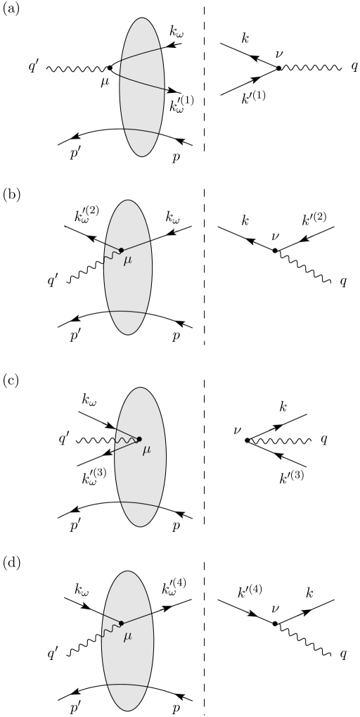
Figure 8: Interpretation of the four terms $\mathcal{M}^{(a,j)}_{s^{\prime}s}(p^{\prime},p,q)$ (41)-(44) where $j=1,\dots,4$ corresponds to (a),…,(d). The shading indicates all possible interactions of the proton with the quarks at the top of the diagrams. The arrows on the lines indicate the interpretation as particle or antiparticle. The orientation of the momentum assignment to the lines is from right to left for all lines, irrespective of the arrows on the lines.

The vertex diagrams on the r.h.s. of figure 8 correspond to the vertex factors $\bar{u}_{r}(k)Z_{q}\gamma^{\nu}v_{r^{\prime}}(k^{\prime(1)})$ etc. in (41)-(44). The diagrams on the l.h.s. of figure 8 correspond to the matrix elements (48)-(60). We emphasise that these are matrix elements for quarks off the energy shell. The normalisations in (48)-(60) are, however, chosen with correct LSZ factors and wave function renormalisation constants in such a way that the matrix elements of $\mathcal{T}^{(a)}$ are finite and would correspond to physical $T$-matrix elements under the following conditions:

• The quarks $q$ are supposed to have a mass shell with a pole mass $m_{q,{\mathrm{pole}}}$ and we choose our mass parameter – which is still at our free disposal – equal to the pole mass. That is, we set $m_{q}=m_{q,{\mathrm{pole}}}$.

• We replace the momenta of the quarks and antiquarks in (48)-(60) – which are in general off the energy shell – by the on-shell momenta. That is we make the replacement $k_{\omega}\to k$, $k_{\omega}^{(1)}\to k^{(1)}$ etc.

Keeping these points in mind we see that figure 8a is clearly interpretable in the dipole picture, in contrast to the other three diagrams. Figure 8b describes the absorption of the photon $q$ on a quark $k^{{\prime}(2)}$ going to quark $k$. This is combined with the amplitude for scattering of quark $k_{\omega}$ on the proton giving quark $k^{{\prime}(2)}_{\omega}$, a photon $q^{\prime}$ and the proton $p^{\prime}$. The interpretation of the figures 8c and 8d is analogous.

A second complication arises when we consider the renormalisation of the photon vertex. We have inserted a wave function renormalisation factor $Z^{-1}_{q}$ in the scattering amplitudes $\mathcal{T}^{(a)}$ (48)-(60), since otherwise they would not be finite. Correspondingly an explicit factor $Z_{q}$ has been put into the splitting function of the initial photon $\gamma(q,\nu)$. Thus we are still dealing with (in general) divergent integrands in (41)-(44) due to the explicit factor $Z_{q}$. This divergence in $Z_{q}$ must, however, be cancelled by a divergence in the integral over $\omega$ and $\mathbf{k}$.

The situation here is similar to the case of overlapping divergences in QED. The way to deal with such overlapping divergences is well known (see for instance [43]). Let $\Gamma^{(q)\nu}(l,l^{\prime})$ be the renormalised $\gamma q\bar{q}$ vertex function. This function satisfies a Dyson-Schwinger equation shown diagrammatically in figure 9, which is obtained as a straightforward generalisation of the corresponding equation in QED, see [43].

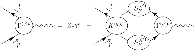
Figure 9: The equation satisfied by the renormalised $\gamma q\bar{q}$ vertex function in diagrammatic form. In the last term a sum over the quark flavour $q^{\prime}$ (see eq. (61)) is implied. The arrows on the lines indicate the interpretation as quark or antiquark.

Here $K^{(q,q^{\prime})}$ is the renormalised kernel of $q^{\prime}\bar{q}^{\prime}$ to $q\bar{q}$ scattering which contains all connected Feynman diagrams which are quark-antiquark two particle irreducible in the $s$-channel and $S^{(q^{\prime})}_{F}$ is the renormalised quark propagator. Since we neglect all higher order terms in the electromagnetic coupling $\alpha_{\rm em}$ the diagram expansion of the kernel comprises only QCD diagrams. Among the diagrams contained in $K^{(q,q^{\prime})}$ is the one-gluon exchange between the quark and antiquark, as well as the annihilation of the quark and antiquark into three gluons in the $s$-channel which then create another quark-antiquark pair (compare the diagram in figure 13 below). In the latter type of diagram the photon can couple to a $q\bar{q}$ pair of a different flavour than the one on the left. This possibility requires the two flavour indices in the notation $K^{(q,q^{\prime})}$.

In a shorthand notation the Dyson-Schwinger equation reads

$$\Gamma^{(q)\nu}(l,l^{\prime})=Z_{q}\gamma^{\nu}-\sum_{q^{\prime}}\int K^{(q,q^{\prime})}S^{(q^{\prime})}_{F}\Gamma^{(q^{\prime})\nu}S^{(q^{\prime})}_{F}\,.$$ (61)

Solving for $Z_{q}\gamma^{\nu}$ we get

$$Z_{q}\gamma^{\nu}=\Gamma^{(q)\nu}(l,l^{\prime})+\sum_{q^{\prime}}\int K^{(q,q^{\prime})}S^{(q^{\prime})}_{F}\Gamma^{(q^{\prime})\nu}S^{(q^{\prime})}_{F}\,.$$ (62)

All quantities on the r.h.s. of this equation are renormalised quantities, in particular, they are finite. The divergence of $Z_{q}$ originates from the integration in the last term. Replacing now $Z_{q}\gamma^{\nu}$ in (41)-(44) according to (62) we get expressions for $\mathcal{M}^{(a,j)}$ for $j=1,\ldots,4$ where all integrands are finite. We still have some freedom how to choose the momenta $l,l^{\prime}$ on the r.h.s. of (62). A natural choice for $\mathcal{M}^{(a,1)}$ is

$$l=k,~{}l^{\prime}=-k^{{\prime}(1)}\,.$$ (63)

With this the final result for $\mathcal{M}^{(a,1)}$ is shown in diagrammatic form in figure 10

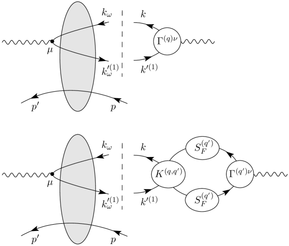
Figure 10: The two terms for the amplitude $\mathcal{M}^{(a,1)}$ (2.4) in diagrammatic form. Again a sum over the quark flavours $q^{\prime}$ is implied in the second term. The arrows on the lines indicate the interpretation as particle or antiparticle. The orientation of the momentum assignment to the lines is from right to left, irrespective of the arrows on the lines.

and reads

$$\mathcal{M}^{(a,1)\mu\nu}_{s^{\prime}s}(p^{\prime},p,q)\! = \!\frac{1}{2\pi}\sum_{q}Q^{2}_{q}\int\frac{d\omega}{\omega+i\epsilon}\int\frac{d^{3}k}{(2\pi)^{3}2k^{0}}(q^{0}-k^{0}-k^{\prime(1)0}-\omega+i\epsilon)^{-1}$$

$${}(2k^{\prime(1)0})^{-1}\sum_{r^{\prime},r}\langle\gamma(q^{\prime},\mu),p(p^{\prime},s^{\prime})|\mathcal{T}^{(a)}|\bar{q}(k^{\prime(1)}_{\omega},r^{\prime}),q(k_{\omega},r),p(p,s)\rangle$$

$${}\bar{u}_{r}(k)\left\{\Gamma^{(q)\nu}(k,-k^{\prime(1)})+\sum_{q^{\prime}}\int K^{(q,q^{\prime})}S^{(q^{\prime})}_{F}\Gamma^{(q^{\prime})\nu}S^{(q^{\prime})}_{F}\right\}v_{r^{\prime}}(k^{\prime(1)})\,.$$

The explicit expressions and diagrammatic forms for $\mathcal{M}^{(a,j)},j=2,3,4$ are analogous and easily constructed. In II we shall study the high energy limit, where we will find that $\mathcal{M}^{(a,1)}$ gives the leading term.

The integrations over $\omega$ and $\mathbf{k}$ (2.4) should be convergent and finite, but only for both terms in the curly brackets inserted together. If we insert for instance only $\Gamma^{(q)\nu}$ a divergence could occur. It would be very interesting to study in detail how the divergences cancel in this equation. It is likely that already a one-loop calculation would reveal the structure of this cancellation, possibly even in a simple model like the abelian gluon model proposed in [44].

For the amplitude ${\cal M}^{(b)}$ corresponding to the generic diagram of figure 2b all the same steps can be performed as for ${\cal M}^{(a)}$. We get again a decomposition as in (36),

$$\mathcal{M}^{(b)\mu\nu}_{s^{\prime}s}(p^{\prime},p,q)=\sum_{j=1}^{4}\mathcal{M}^{(b,j)\mu\nu}_{s^{\prime}s}(p^{\prime},p,q)\,,$$ (65)

where of these four terms the important term at high energies is

$$\mathcal{M}^{(b,1)\mu\nu}_{s^{\prime}s}(p^{\prime},p,q)\! = \!\frac{1}{2\pi}\sum_{q^{\prime\prime},q}Q_{q^{\prime\prime}}Q_{q}\int\frac{d\omega}{\omega+i\epsilon}\int\frac{d^{3}k}{(2\pi)^{3}2k^{0}}(q^{0}-k^{0}-k^{\prime(1)0}-\omega+i\epsilon)^{-1}$$

$${}\!(2k^{\prime(1)0})^{-1}\sum_{r^{\prime},r}\langle\gamma(q^{\prime},\mu),p(p^{\prime},s^{\prime})|\mathcal{T}^{(q^{\prime\prime},b)}|\bar{q}(k^{\prime(1)}_{\omega},r^{\prime}),q(k_{\omega},r),p(p,s)\rangle$$

$${}\!\bar{u}_{r}(k)\left\{\Gamma^{(q)\nu}(k,-k^{\prime(1)})+\sum_{q^{\prime}}\int K^{(q,q^{\prime})}S^{(q^{\prime})}_{F}\Gamma^{(q^{\prime})\nu}S^{(q^{\prime})}_{F}\right\}v_{r^{\prime}}(k^{\prime(1)})\,.$$

Graphically this is represented in figure 11.

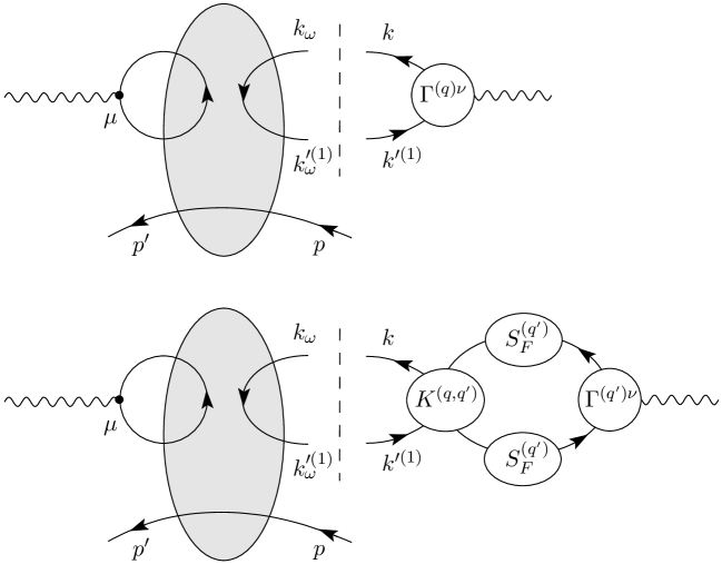
Figure 11: The two terms for the amplitude $\mathcal{M}^{(b,1)}$ (2.4) in diagrammatic form. The interpretation of the lines is as in figure 10.

The explicit expressions are given in appendix C. The matrix element $\langle\gamma,p|\mathcal{T}^{(q^{\prime\prime},b)}|\bar{q},q,p\rangle$ in (2.4) represents the scattering of a $q\bar{q}$ dipole on a proton giving a photon component $\bar{q}^{\prime\prime}\gamma^{\mu}q^{\prime\prime}$ and a proton.

It is instructive to illustrate the overlapping divergences problem which is solved by (2.4) and (2.4) with two simple perturbative diagrams. Consider first the diagram of figure 12.

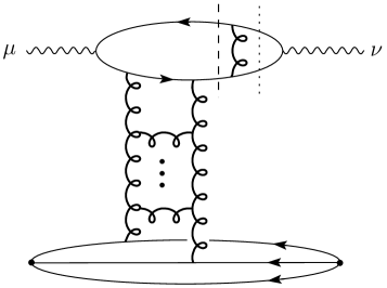
Figure 12: Perturbative diagram contributing to the amplitude $\mathcal{M}^{(a,1)}$

Cutting this diagram along the dashed line gives a higher order correction to the photon vertex function. Cutting it along the dotted line we find a higher order correction to the scattering amplitude of the colour dipole on the proton. In the expression (2.4) both corrections are taken into account and the ‘double counting’ problem is exactly taken care of by the kernel term $K^{(q,q^{\prime})}$.

This double counting or overlapping divergences problem in the ‘cut’ diagrams and its solution in (2.4) and (2.4) also ‘mixes’ the diagrams of figures 2a and 2b. This is despite the fact that these diagram classes are clearly identifiable and do not mix at the starting level. Indeed, consider figure 13, which is clearly a diagram of type 2b, and cut the diagram first along the dotted line.

Figure 13: Perturbative diagram contributing to the amplitude $\mathcal{M}^{(a,1)}$ but also to $\mathcal{M}^{(b,1)}$

Then we have a colour dipole-proton amplitude of type 2b with a simple vertex on the photon side. Cutting along the dashed line, we can interpret it as a colour dipole-proton amplitude of type 2a with a vertex correction on the photon side. This shows that great care has to be exercised when cutting perturbative diagrams and trying to interpret them in terms of colour dipole amplitude times photon wave function. We would like to stress that the original classification of diagram types in figure 2 is not affected by this. The ‘mixing’ of diagram classes comes into play only when one considers cut diagrams, and then an individual diagram like the one in figure 13 can be associated with higher order corrections occurring to the left or to the right from the cut, depending on the position of the cut.

Finally we want to make some remarks concerning the outgoing photon. As we indicate briefly in appendix A one can treat the outgoing photon $\gamma(q^{\prime},\mu)$ of the Compton amplitude in complete analogy to the incoming photon $\gamma(q,\nu)$, performing all the steps we have done for the incoming photon in the same manner, including the renormalisation of the the photon vertex via its Dyson-Schwinger equation. The resulting expressions would in their form be completely symmetric in the incoming and outgoing photon. For the purpose of the present papers, especially for the study of the high energy limit to be discussed in II, it will however be sufficient to treat only the incoming photon in this way.

3 Summary

In the present paper we have studied the real and virtual Compton amplitude for photon-nucleon scattering in a nonperturbative framework. We have classified the different contributions to the amplitude according to their quark line skeleton. We have discussed the relative magnitude of the different contributions and have identified the two contributions $\mathcal{M}^{(a)}$ and $\mathcal{M}^{(b)}$ represented by figures 2a and 2b as the leading ones at high energies. Concentrating on these two contributions we have then inserted on the quark lines after the incoming photon vertex suitable factors of one, given by the free Dirac operator acting on the free quark propagator for a chosen mass $m_{q}$. After integrating by parts we have used spin times colour sum decompositions for the free quark propagators to obtain expressions which bring us closer to the dipole picture of high energy scattering. For both amplitudes $\mathcal{M}^{(a)}$ and $\mathcal{M}^{(b)}$ we obtained four terms where in each case only one had the structure of a vertex function describing the splitting of the photon into a $q\bar{q}$ pair convoluted with a scattering amplitude for an off energy shell $q\bar{q}$ pair on the proton. The results for these parts of the amplitudes $\mathcal{M}^{(a)}$ and $\mathcal{M}^{(b)}$ are given in (2.4) and (2.4), respectively, see figures 10 and 11. In II these results will allow us to isolate the leading term in the high energy limit. A key point in the present paper is that we have taken into account the renormalisation of the photon-quark-antiquark vertex. We find that the renormalisation induces an important rescattering correction which is usually not taken into account in the dipole picture.

From the contribution of figure 2a we will be able to obtain the usual dipole picture of photon-proton scattering after suitable further approximations. We will in fact show that this is the leading term at high energies and large photon virtualities. We find, however, that there are two important correction terms which can potentially become large at small photon virtualities, that is in the interesting transition region from the perturbative to the nonperturbative regime. The first correction comes from the rescattering of the quark and antiquark into which the virtual photon splits, the second correction comes from the contribution of figure 2b. Both of them are suppressed only at large photon virtualities but not due to large energies.

The motivation for the dipole picture of high energy scattering is closely related to the notion of light-cone wave functions, see for example [45, 46]. When applied to a real or virtual photon this concept naturally suggests to include in addition to the quark-antiquark component also higher Fock states of the photon like for example the quark-antiquark-gluon component of the wave function etc., and to sum the amplitudes for the scattering of these components off the proton. Also the perturbative framework can be arranged according to this view. We emphasise that in our treatment nothing is missing and, in particular, higher Fock states do not and should not occur explicitly here. Recall in this context that the solution of the overlapping divergences problem for the vacuum polarisation in QED (see [43]) also does not involve analogues of higher Fock states for the photon. Nevertheless we think that it is an interesting problem for further investigations to try to see where and how the various terms of a Fock state expansion of the photon as discussed for instance in [33] can be identified in our approach.

In the second paper we will discuss in detail the high energy limit of the expressions (2.4) and (2.4) obtained here from the contributions of figures 2a and 2b. We will also study the problem of gauge invariance. In particular, we will discuss whether different parts of the amplitude are separately gauge invariant. We point out the consequences of this issue for the correct definition of the perturbative wave function of the photon. Finally we derive some phenomenological consequences of the simple dipole picture which can help to find its range of validity. With this brief outlook we want to close the present paper, further conclusions will be presented in the second paper.

Appendix A Propagators and decomposition of the Compton amplitude

In this appendix we give the derivation of the analytic expressions for the diagrams of figure 2. We start with the Lagrangian of QCD

$${\cal L}_{\mbox{\scriptsize QCD}}(x)=-\frac{1}{2}\mathrm{Tr}\left(G_{\lambda\rho}(x)G^{\lambda\rho}(x)\right)+\sum_{q}\bar{q}(x)(i\gamma^{\lambda}D_{\lambda}-m^{(0)}_{q})q(x)\,,$$ (A.1)

where $G_{\lambda\rho}$ is the matrix-valued gluon field strength tensor and $D_{\lambda}$ the covariant derivative (for the notation see [36]):

$$G_{\lambda\rho}(x) = \left(\partial_{\lambda}G^{a}_{\rho}(x)-\partial_{\rho}G^{a}_{\lambda}(x)-g^{(0)}f_{abc}G^{b}_{\lambda}(x)G^{c}_{\rho}(x)\right)\frac{\lambda_{a}}{2}\,,$$ (A.2)

$$D_{\lambda}q(x) = \left(\partial_{\lambda}+ig^{(0)}G^{a}_{\lambda}\frac{\lambda_{a}}{2}\right)q(x)\,.$$ (A.3)

Here $g^{(0)}$ is the bare coupling parameter and $m^{(0)}_{q}$ are the bare quark masses. Since ${\cal L}_{\mbox{\scriptsize QCD}}$ is bilinear in the quark fields we can immediately perform the $q$ and $\bar{q}$ functional integrals in (2.1). To write the result in a concise form we use the quark propagator $S^{(q)}_{F}(x,y;G)$ for given gluon potential, see (19). This propagator satisfies Lippmann-Schwinger relations. Let $S_{F}^{(q,0)}$ be the free propagator for mass $m_{q}$ (see (27), (28)). Then we have in matrix notation

$$S_{F}^{(q)}(G) = S_{F}^{(q,0)}-S_{F}^{(q,0)}\left(g^{(0)}\not\!G^{a}\frac{\lambda_{a}}{2}+m_{q}^{(0)}-m_{q}\right)S_{F}^{(q)}(G)$$ (A.4)

$$= S_{F}^{(q,0)}-S_{F}^{(q)}(G)\left(g^{(0)}\not\!G^{a}\frac{\lambda_{a}}{2}+m_{q}^{(0)}-m_{q}\right)S_{F}^{(q,0)}\,.$$

From (A.4) we get

$$S_{F}^{(q)}(x,y;G)\left(i\!\stackrel{{\scriptstyle\leftarrow}}{{\not\!\!D}}_{y}+m_{q}^{(0)}\right) = S_{F}^{(q)}(x,y;G)\left(i\!\stackrel{{\scriptstyle\leftarrow}}{{\!\not\!\partial}}_{y}+g^{(0)}\not\!G^{a}\frac{\lambda_{a}}{2}+m_{q}^{(0)}\right)$$ (A.5)

$$= \delta^{(4)}(x-y)\,.$$

We define the contraction of two quark fields of flavour $q$ as

$$\mathop{\vbox{\halign{#\cr\kern 1.72218pt\cr$\hbox{$\hskip 2.41145pt\vrule height=3.65973pt,width=0.29999pt,depth=2.52737pt\kern-0.29999pt\vrule height=3.65973pt,width=18.40453pt,depth=-3.35974pt\kern-0.29999pt\vrule height=3.65973pt,width=0.29999pt,depth=1.15515pt$\hss}$\crcr\kern 1.72218pt\nointerlineskip\cr\hbox{$\displaystyle{}{q}{(x)}{\overline{q}}(y)=\frac{1}{i}S^{(q)}_{F}(x,y;G)$}\crcr}}}\limits$$ (A.6)

and represent it by a line in our diagrams:

In a functional integral over gluon and quark degrees of freedom we then have to contract all quark fields in all possible ways and integrate over the remaining gluon degrees of freedom including the fermion determinant. Schematically we have:

$$\Big{\langle}\ldots q(x)\bar{q}(y)\ldots\Big{\rangle}_{G,q,\bar{q}} = \Big{\langle}\ldots\frac{1}{i}S^{(q)}_{F}(x,y;G)\ldots\Big{\rangle}_{G}$$ (A.7)

$$+\,\textup{all other contractions of quark fields.}$$

Here the functional integral on the l.h.s. is defined in (11), (12), that on the r.h.s. in (20), (21). For the functional integral in (2.1) (there written already for $x^{\prime}=0$) we find in this way

$$\Big{\langle}\psi_{p}(y^{\prime})J^{\mu}(x^{\prime})J^{\nu}(x)\overline{\psi}_{p}(y)\Big{\rangle}_{G,q,\bar{q}}=$$ (A.8)

$$= \sum_{q^{\prime},q}Q_{q^{\prime}}Q_{q}\Big{\langle}\Gamma_{\alpha^{\prime}\beta^{\prime}\gamma^{\prime}}u_{\alpha^{\prime}}(y^{\prime})u_{\beta^{\prime}}(y^{\prime})d_{\gamma^{\prime}}(y^{\prime})\bar{q}^{\prime}(x^{\prime})\gamma^{\mu}q^{\prime}(x^{\prime})\bar{q}(x)\gamma^{\nu}q(x)$$

$$\hskip 56.9055pt\bar{\Gamma}_{\alpha\beta\gamma}\bar{d}_{\gamma}(y)\bar{u}_{\beta}(y)\bar{u}_{\alpha}(y)\Big{\rangle}_{G,q,\bar{q}}$$

$$= \mathcal{J}^{(a)}+\ldots+\mathcal{J}^{(g)}\,.$$

The integration over quark and antiquark fields gives rise to a number of terms in which these fields are contracted in all possible ways. The resulting propagators can be understood as defining a quark line skeleton for the graphical representation of the respective term. We have classified the different types of diagrams in figure 2, and the terms $\mathcal{J}^{(a)}$ to $\mathcal{J}^{(g)}$ in the last line above are defined as corresponding to this classification.

Inserting the expression (A.8) in (2.1) leads to the decomposition of the amplitude in (13) with

$$\mathcal{M}^{(a)\mu\nu}_{s^{\prime}s}(p^{\prime},p,q) = -\frac{i}{2\pi m_{p}Z_{p}}\int d^{4}y^{\prime}~{}d^{4}y\,e^{ip^{\prime}y^{\prime}}\bar{u}_{s^{\prime}}(p^{\prime})(-i\!\stackrel{{\scriptstyle\rightarrow}}{{\!\not\!\partial}}_{y^{\prime}}+m_{p})$$ (A.9)

$$\int d^{4}x\,e^{-iqx}\left.{\cal J}^{(a)}\right|_{x^{\prime}=0}(i\!\stackrel{{\scriptstyle\leftarrow}}{{\!\not\!\partial}}_{y}+m_{p})u_{s}(p)e^{-ipy}\,,$$

and ${\cal M}^{(b)}$ to ${\cal M}^{(g)}$ are related to $\mathcal{J}^{(a)},\ldots,\mathcal{J}^{(g)}$ in a completely analogous way. The expressions $\mathcal{J}^{(a)},\ldots,\mathcal{J}^{(g)}$ for $x^{\prime}=0$ are represented in diagrammatic language in figure 2. The general rule is that for each quark line in a diagram in figure 2 one has to insert a factor $-iS^{(q)}_{F}(x,y;G)$ according to (A.6). The vertices with the photon just represent the coupling $\gamma^{\nu}Q_{q}$. The functional integral $\langle~{}\rangle_{G}$ as defined in (20) has to be performed over the integrand resulting in this way. This is indicated by the shading in figures 2a to 2g. The explicit expressions are

$$\mathcal{J}^{(a)}=\sum_{q}Q^{2}_{q}\Bigg{\langle}\mathop{\vbox{\halign{#\cr\kern 1.72218pt\cr$\hbox{$\hskip 3.25696pt\vrule height=7.31946pt,width=0.29999pt,depth=-0.11153pt\kern-0.29999pt\vrule height=7.31946pt,width=23.15385pt,depth=-7.01947pt\kern-0.29999pt\vrule height=7.31946pt,width=0.29999pt,depth=1.15515pt$\hss}$\crcr\kern 1.72218pt\nointerlineskip\cr\hbox{$\displaystyle{}{\psi}{{}_{p}(y^{\prime})}{\overline{\psi}}_{p}(y)$}\crcr}}}\limits(-1)\mathrm{Tr}\left[\gamma^{\mu}\frac{1}{i}S_{F}^{(q)}(x^{\prime},x;G)\gamma^{\nu}\frac{1}{i}S_{F}^{(q)}(x,x^{\prime};G)\right]\Bigg{\rangle}_{G}\,,$$ (A.10)

where

$$\mathop{\vbox{\halign{#\cr\kern 1.72218pt\cr$\hbox{$\hskip 3.25696pt\vrule height=7.31946pt,width=0.29999pt,depth=-0.11153pt\kern-0.29999pt\vrule height=7.31946pt,width=23.15385pt,depth=-7.01947pt\kern-0.29999pt\vrule height=7.31946pt,width=0.29999pt,depth=1.15515pt$\hss}$\crcr\kern 1.72218pt\nointerlineskip\cr\hbox{$\displaystyle{}{\psi}{{}_{p}(y^{\prime})}{\overline{\psi}}_{p}(y)$}\crcr}}}\limits = \Gamma_{\alpha^{\prime}\beta^{\prime}\gamma^{\prime}}\bar{\Gamma}_{\alpha\beta\gamma}\,\frac{1}{i}S^{(d)}_{F\gamma^{\prime}\gamma}(y^{\prime},y;G)$$ (A.14)

$${}\biggl{\{}\frac{1}{i}S^{(u)}_{F\beta^{\prime}\beta}(y^{\prime},y;G)\frac{1}{i}S^{(u)}_{F\alpha^{\prime}\alpha}(y^{\prime},y;G)-(\alpha\leftrightarrow\beta)\biggr{\}}\,,$$

further

$$\mathcal{J}^{(b)}=\sum_{q^{\prime},q}Q_{q^{\prime}}Q_{q}\Bigg{\langle}\mathop{\vbox{\halign{#\cr\kern 1.72218pt\cr$\hbox{$\hskip 3.25696pt\vrule height=7.31946pt,width=0.29999pt,depth=-0.11153pt\kern-0.29999pt\vrule height=7.31946pt,width=23.15385pt,depth=-7.01947pt\kern-0.29999pt\vrule height=7.31946pt,width=0.29999pt,depth=1.15515pt$\hss}$\crcr\kern 1.72218pt\nointerlineskip\cr\hbox{$\displaystyle{}{\psi}{{}_{p}(y^{\prime})}{\overline{\psi}}_{p}(y)$}\crcr}}}\limits\mathrm{Tr}\left[\gamma^{\mu}\frac{1}{i}S_{F}^{(q^{\prime})}(x^{\prime},x^{\prime};G)\right]\mathrm{Tr}\left[\gamma^{\nu}\frac{1}{i}S^{(q)}_{F}(x,x;G)\right]\Bigg{\rangle}_{G}\,,$$ (A.15)

and

$$\mathcal{J}^{(c)}=\Gamma_{\alpha^{\prime}\beta^{\prime}\gamma^{\prime}}\bar{\Gamma}_{\alpha\beta\gamma}\Bigg{\langle}Q^{2}_{d}\left[\frac{1}{i}S^{(d)}_{F}(y^{\prime},x^{\prime};G)\gamma^{\mu}\frac{1}{i}S^{(d)}_{F}(x^{\prime},x;G)\gamma^{\nu}\frac{1}{i}S^{(d)}_{F}(x,y;G)\right]_{\gamma^{\prime}\gamma}$$ (A.16)

$${}\hskip 8.5359pt\left[\frac{1}{i}S^{(u)}_{F\beta^{\prime}\beta}(y^{\prime},y;G)\frac{1}{i}S^{(u)}_{F\alpha^{\prime}\alpha}(y^{\prime},y;G)-(\alpha\leftrightarrow\beta)\right]$$

$${}+Q^{2}_{u}\frac{1}{i}S^{(d)}_{F\gamma^{\prime}\gamma}(y^{\prime},y;G)$$

$${}\hskip 8.5359pt\biggl{\{}\left[\frac{1}{i}S^{(u)}_{F}(y^{\prime},x^{\prime};G)\gamma^{\mu}\frac{1}{i}S^{(u)}_{F}(x^{\prime},x;G)\gamma^{\nu}\frac{1}{i}S^{(u)}_{F}(x,y;G)\right]_{\beta^{\prime}\beta}\frac{1}{i}S^{(u)}_{F\alpha^{\prime}\alpha}(y^{\prime},y;G)$$

$${}\hskip 8.5359pt-(\alpha^{\prime}\leftrightarrow\beta^{\prime})-(\alpha\leftrightarrow\beta)+(\alpha\leftrightarrow\beta,\alpha^{\prime}\leftrightarrow\beta^{\prime})\biggr{\}}\Bigg{\rangle}_{G}\,.$$

${\cal J}^{(d)}$ is as ${\cal J}^{(c)}$ but with $\mu\leftrightarrow\nu$ and $x\leftrightarrow x^{\prime}$. Explicitly,

$$\mathcal{J}^{(d)}=\Gamma_{\alpha^{\prime}\beta^{\prime}\gamma^{\prime}}\bar{\Gamma}_{\alpha\beta\gamma}\Bigg{\langle}Q^{2}_{d}\left[\frac{1}{i}S^{(d)}_{F}(y^{\prime},x;G)\gamma^{\nu}\frac{1}{i}S^{(d)}_{F}(x,x^{\prime};G)\gamma^{\mu}\frac{1}{i}S^{(d)}_{F}(x^{\prime},y;G)\right]_{\gamma^{\prime}\gamma}$$ (A.17)

$${}\hskip 8.5359pt\left[\frac{1}{i}S^{(u)}_{F\beta^{\prime}\beta}(y^{\prime},y;G)\frac{1}{i}S^{(u)}_{F\alpha^{\prime}\alpha}(y^{\prime},y;G)-(\alpha\leftrightarrow\beta)\right]$$

$${}+Q^{2}_{u}\frac{1}{i}S^{(d)}_{F\gamma^{\prime}\gamma}(y^{\prime},y;G)$$

$${}\hskip 8.5359pt\biggl{\{}\left[\frac{1}{i}S^{(u)}_{F}(y^{\prime},x;G)\gamma^{\nu}\frac{1}{i}S^{(u)}_{F}(x,x^{\prime};G)\gamma^{\mu}\frac{1}{i}S^{(u)}_{F}(x^{\prime},y;G)\right]_{\beta^{\prime}\beta}\frac{1}{i}S^{(u)}_{F\alpha^{\prime}\alpha}(y^{\prime},y;G)$$

$${}\hskip 8.5359pt-(\alpha^{\prime}\leftrightarrow\beta^{\prime})-(\alpha\leftrightarrow\beta)+(\alpha\leftrightarrow\beta,\alpha^{\prime}\leftrightarrow\beta^{\prime})\biggr{\}}\Bigg{\rangle}_{G}\,.$$

We further have

$$\mathcal{J}^{(e)}=\Gamma_{\alpha^{\prime}\beta^{\prime}\gamma^{\prime}}\bar{\Gamma}_{\alpha\beta\gamma}\Bigg{\langle}\bigg{\{}Q^{2}_{u}\frac{1}{i}S^{(d)}_{F\gamma^{\prime}\gamma}(y^{\prime},y;G)$$ (A.18)

$${}\bigg{[}\left(\frac{1}{i}S^{(u)}_{F}(y^{\prime},x;G)\gamma^{\nu}\frac{1}{i}S^{(u)}_{F}(x,y;G)\right)_{\alpha^{\prime}\alpha}\left(\frac{1}{i}S^{(u)}_{F}(y^{\prime},x^{\prime};G)\gamma^{\mu}\frac{1}{i}S^{(u)}_{F}(x^{\prime},y;G)\right)_{\beta^{\prime}\beta}$$

$${}-(\alpha^{\prime}\leftrightarrow\beta^{\prime})-(\alpha\leftrightarrow\beta)+(\alpha^{\prime}\leftrightarrow\beta^{\prime},\alpha\leftrightarrow\beta)\bigg{]}$$

$${}+Q_{u}Q_{d}\bigg{[}\left(\frac{1}{i}S^{(d)}_{F}(y^{\prime},x^{\prime};G)\gamma^{\mu}\frac{1}{i}S^{(d)}_{F}(x^{\prime},y;G)\right)_{\gamma^{\prime}\gamma}$$

$${}\hskip 46.94687pt\left(\frac{1}{i}S^{(u)}_{F}(y^{\prime},x;G)\gamma^{\nu}\frac{1}{i}S^{(u)}_{F}(x,y;G)\right)_{\alpha^{\prime}\alpha}\frac{1}{i}S^{(u)}_{F\,\beta^{\prime}\beta}(y^{\prime},y;G)$$

$${}\hskip 46.94687pt-(\alpha^{\prime}\leftrightarrow\beta^{\prime})-(\alpha\leftrightarrow\beta)+(\alpha^{\prime}\leftrightarrow\beta^{\prime},\alpha\leftrightarrow\beta)\bigg{]}$$

$${}+Q_{u}Q_{d}\bigg{[}\left(\frac{1}{i}S^{(d)}_{F}(y^{\prime},x;G)\gamma^{\nu}\frac{1}{i}S^{(d)}_{F}(x,y;G)\right)_{\gamma^{\prime}\gamma}$$

$${}\hskip 46.94687pt\left(\frac{1}{i}S^{(u)}_{F}(y^{\prime},x^{\prime};G)\gamma^{\mu}\frac{1}{i}S^{(u)}_{F}(x^{\prime},y;G)\right)_{\alpha^{\prime}\alpha}\frac{1}{i}S^{(u)}_{F\,\beta^{\prime}\beta}(y^{\prime},y;G)$$

$${}\hskip 46.94687pt-(\alpha^{\prime}\leftrightarrow\beta^{\prime})-(\alpha\leftrightarrow\beta)+(\alpha^{\prime}\leftrightarrow\beta^{\prime},\alpha\leftrightarrow\beta)\bigg{]}\biggr{\}}\Bigg{\rangle}_{G}\,,$$

$$\mathcal{J}^{(f)}=\Gamma_{\alpha^{\prime}\beta^{\prime}\gamma^{\prime}}\bar{\Gamma}_{\alpha\beta\gamma}\Bigg{\langle}\bigg{[}\sum_{q^{\prime}}Q_{q^{\prime}}(-1)\mathrm{Tr}\left(\gamma^{\mu}\frac{1}{i}S_{F}^{(q^{\prime})}(x^{\prime},x^{\prime};G)\right)\bigg{]}$$ (A.19)

$${}\bigg{\{}Q_{u}\frac{1}{i}S^{(d)}_{F\gamma^{\prime}\gamma}(y^{\prime},y;G)\bigg{[}\left(\frac{1}{i}S^{(u)}_{F}(y^{\prime},x;G)\gamma^{\nu}\frac{1}{i}S^{(u)}_{F}(x,y;G)\right)_{\alpha^{\prime}\alpha}\frac{1}{i}S^{(u)}_{F\beta^{\prime}\beta}(y^{\prime},y;G)$$

$${}-(\alpha^{\prime}\leftrightarrow\beta^{\prime})-(\alpha\leftrightarrow\beta)+(\alpha^{\prime}\leftrightarrow\beta^{\prime},\alpha\leftrightarrow\beta)\bigg{]}$$

$${}+Q_{d}\bigg{(}\frac{1}{i}S^{(d)}_{F}(y^{\prime},x;G)\gamma^{\nu}\frac{1}{i}S^{(d)}_{F}(x,y;G)\bigg{)}_{\gamma^{\prime}\gamma}$$

$${}\bigg{[}\frac{1}{i}S^{(u)}_{F\alpha^{\prime}\alpha}(y^{\prime},y;G)\frac{1}{i}S^{(u)}_{F\beta^{\prime}\beta}(y^{\prime},y;G)-(\alpha\leftrightarrow\beta)\bigg{]}\bigg{\}}\Bigg{\rangle}_{G}\,,$$

$$\mathcal{J}^{(g)}=\Gamma_{\alpha^{\prime}\beta^{\prime}\gamma^{\prime}}\bar{\Gamma}_{\alpha\beta\gamma}\Bigg{\langle}\bigg{[}\sum_{q}Q_{q}(-1)\mathrm{Tr}\left(\gamma^{\nu}\frac{1}{i}S_{F}^{(q)}(x,x;G)\right)\bigg{]}$$ (A.20)

$${}\bigg{\{}Q_{u}\frac{1}{i}S^{(d)}_{F\gamma^{\prime}\gamma}(y^{\prime},y;G)\bigg{[}\left(\frac{1}{i}S^{(u)}_{F}(y^{\prime},x^{\prime};G)\gamma^{\mu}\frac{1}{i}S^{(u)}_{F}(x^{\prime},y;G)\right)_{\alpha^{\prime}\alpha}\frac{1}{i}S^{(u)}_{F\beta^{\prime}\beta}(y^{\prime},y;G)$$

$${}-(\alpha^{\prime}\leftrightarrow\beta^{\prime})-(\alpha\leftrightarrow\beta)+(\alpha^{\prime}\leftrightarrow\beta^{\prime},\alpha\leftrightarrow\beta)\bigg{]}$$

$${}+Q_{d}\bigg{(}\frac{1}{i}S^{(d)}_{F}(y^{\prime},x^{\prime};G)\gamma^{\mu}\frac{1}{i}S^{(d)}_{F}(x^{\prime},y;G)\bigg{)}_{\gamma^{\prime}\gamma}$$

$${}\bigg{[}\frac{1}{i}S^{(u)}_{F\alpha^{\prime}\alpha}(y^{\prime},y;G)\frac{1}{i}S^{(u)}_{F\beta^{\prime}\beta}(y^{\prime},y;G)-(\alpha\leftrightarrow\beta)\bigg{]}\bigg{\}}\Bigg{\rangle}_{G}\,.$$

Finally, we indicate how we can make an analysis of the amplitude (2.1) treating incoming and outgoing photons in a symmetric way. Using translational invariance of the functional integral we can write (2.1) also as follows

$$\mathcal{M}^{\mu\nu}_{s^{\prime}s}(p^{\prime},p,q)=-\frac{i}{2\pi m_{p}Z_{p}}\int d^{4}y\,d^{4}x^{\prime}\,d^{4}x\bigg{[}\bar{u}_{s^{\prime}}(p^{\prime})(-i\!\stackrel{{\scriptstyle\rightarrow}}{{\!\not\!\partial}}_{y^{\prime}}+m_{p})$$ (A.21)

$${}\left\langle\psi_{p}(y^{\prime})e^{iq^{\prime}x^{\prime}}J^{\mu}(x^{\prime})e^{-iqx}J^{\nu}(x)\overline{\psi}_{p}(y)\right\rangle_{G,q,\bar{q}}(i\!\stackrel{{\scriptstyle\leftarrow}}{{\!\not\!\partial}}_{y}+m_{p})u_{s}(p)e^{-ipy}\left.\bigg{]}\right|_{y^{\prime}=0}\,.\,\,\,\,$$

Inserting here the decomposition (A.8) of the functional integral we obtain

$$\mathcal{M}^{(a)\mu\nu}_{s^{\prime}s}(p^{\prime},p,q) = -\frac{i}{2\pi m_{p}Z_{p}}\int d^{4}y\,d^{4}x^{\prime}\,d^{4}x\,e^{iq^{\prime}x^{\prime}}e^{-iqx}e^{-ipy}$$ (A.22)

$${}\bar{u}_{s^{\prime}}(p^{\prime})(-i\!\stackrel{{\scriptstyle\rightarrow}}{{\!\not\!\partial}}_{y^{\prime}}+m_{p})\left.\mathcal{J}^{(a)}(i\!\stackrel{{\scriptstyle\leftarrow}}{{\!\not\!\partial}}_{y}+m_{p})u_{s}(p)\right|_{y^{\prime}=0}\,,$$

and similarly for $\mathcal{M}^{(b)},\dots,\mathcal{M}^{(g)}$. With (A.10) we now find

$$\mathcal{M}^{(a)\mu\nu}_{s^{\prime}s}(p^{\prime},p,q) = -\frac{i}{2\pi m_{p}Z_{p}}\int d^{4}y\bigg{[}\bar{u}_{s^{\prime}}(p^{\prime})(-i\!\stackrel{{\scriptstyle\rightarrow}}{{\!\not\!\partial}}_{y^{\prime}}+m_{p})$$ (A.26)

$${}\sum_{q}Q_{q}^{2}\Big{\langle}\mathop{\vbox{\halign{#\cr\kern 1.72218pt\cr$\hbox{$\hskip 3.25696pt\vrule height=7.31946pt,width=0.29999pt,depth=-0.11153pt\kern-0.29999pt\vrule height=7.31946pt,width=23.15385pt,depth=-7.01947pt\kern-0.29999pt\vrule height=7.31946pt,width=0.29999pt,depth=1.15515pt$\hss}$\crcr\kern 1.72218pt\nointerlineskip\cr\hbox{$\displaystyle{}{\psi}{{}_{p}(y^{\prime})}{\overline{\psi}}_{p}(y)$}\crcr}}}\limits\tilde{A}^{(q)\mu\nu}(q^{\prime},q)\Big{\rangle}_{G}(i\!\stackrel{{\scriptstyle\leftarrow}}{{\!\not\!\partial}}_{y}+m_{p})u_{s}(p)e^{-ipy}\left.\bigg{]}\right|_{y^{\prime}=0}\,,$$

where

$$\tilde{A}^{(q)\mu\nu}(q^{\prime},q) = \int d^{4}x^{\prime}\,d^{4}x\,\mathrm{Tr}\left[e^{iq^{\prime}x^{\prime}}\gamma^{\mu}S^{(q)}_{F}(x^{\prime},x;G)e^{-iqx}\gamma^{\nu}S^{(q)}_{F}(x,x^{\prime};G)\right]\,.\hskip 8.5359pt$$ (A.27)

The further analysis of $\tilde{A}^{(q)\mu\nu}$ can then be done exactly as for $A^{(q)\mu\nu}$ of (18) in section 2.3. The representation (A.26), (A.27) for the amplitude then also allows the treatment of the final state photon $\gamma(q^{\prime},\mu)$ in the same way as the initial state photon, that is replacing it by a dipole in the way explained in section 2.

Appendix B Decomposition using spin sums

The free quark propagator for mass $m_{q}$ can be written as follows

$$S^{(q,0)}_{F}(x,y) = -\int\frac{d^{4}k}{(2\pi)^{4}}\,e^{-ik(x-y)}\frac{\not\!k+m_{q}}{k^{2}-m^{2}_{q}+i\epsilon}\,\mathbf{1}_{3}$$ (B.1)

$$= \theta(x^{0}-y^{0})\frac{i}{(2\pi)^{3}}\int\frac{d^{3}k}{2k^{0}}\,e^{-ik(x-y)}(\not\!k+m_{q})\,\mathbf{1}_{3}$$

$${}+\theta(y^{0}-x^{0})\frac{i}{(2\pi)^{3}}\int\frac{d^{3}k}{2k^{0}}\,e^{ik(x-y)}(-\not\!k+m_{q})\,\mathbf{1}_{3}\,,$$

where $k^{0}=(\mathbf{k}^{2}+m^{2}_{q})^{1/2}$, and $\mathbf{1}_{3}$ is the unit matrix in colour space. We define the Dirac times colour spinors as

$$u_{r}(k) = u_{\lambda}(k)\,\mathbf{e}_{A}\,,$$ (B.2)

$$v_{r}(k) = v_{\lambda}(k)\,\mathbf{e}_{A}\,.$$ (B.3)

Here $r=(\lambda,A)$ are the spin times colour indices with $\lambda\in\{1/2,-1/2\}$ and $A\in\{1,2,3\}$. $u_{\lambda}(k)$ and $v_{\lambda}(k)$ are the usual Dirac spinors for mass $m_{q}$, and $\mathbf{e}_{A}$ are orthonormal basis vectors in colour space. We then have for the spin and colour sums

$$\sum_{r}u_{r}(k)\bar{u}_{r}(k) = (\not\!k+m_{q})\,\mathbf{1}_{3}\,,$$ (B.4)

$$\sum_{r}v_{r}(k)\bar{v}_{r}(k) = (\not\!k-m_{q})\,\mathbf{1}_{3}\,.$$ (B.5)

Inserting this and the Fourier representations for the $\theta$-functions in (B.1) we get

$$S^{(q,0)}_{F}(x,y) = -\frac{1}{2\pi}\int^{\infty}_{-\infty}\frac{d\omega}{\omega+i\epsilon}\int\frac{d^{3}k}{(2\pi)^{3}2k^{0}}$$ (B.6)

$${}\sum_{r}\left\{e^{-ik_{\omega}x}u_{r}(k)\bar{u}_{r}(k)e^{ik_{\omega}y}-e^{ik_{\omega}x}v_{r}(k)\bar{v}_{r}(k)e^{-ik_{\omega}y}\right\}\,.$$

Here

$$k = \left(\begin{array}[]{c}k^{0}\\ \mathbf{k}\end{array}\right),$$ (B.9)

$$k_{\omega} = \left(\begin{array}[]{c}k^{0}+\omega\\ \mathbf{k}\end{array}\right)\,.$$ (B.12)

We find it convenient to introduce matrix notation. For this we define

$$(x|k_{\omega},r) = u_{r}(k)e^{-ik_{\omega}x}\,,$$

$$(k_{\omega},r|x) = e^{ik_{\omega}x}\bar{u}_{r}(k)\,,$$

$$(x|\overline{k_{\omega},r}) = v_{r}(k)e^{ik_{\omega}x}\,,$$

$$(\overline{k_{\omega},r}|x) = e^{-ik_{\omega}x}\bar{v}_{r}(k)\,.$$ (B.13)

We also use the summation convention for spin times colour indices and momenta, implying integration over two identical momenta $k$ with the usual invariant phase space measure. Note that this measure contains the energy denominator $k^{0}$ and not $k_{\omega}^{0}$. To give an example we write

$$(x|k_{\omega},r)(k_{\omega},r|y)=\sum_{r}\int\frac{d^{3}k}{(2\pi)^{3}2k^{0}}\,e^{-ik_{\omega}x}u_{r}(k)\bar{u}_{r}(k)e^{ik_{\omega}y}\,.$$ (B.14)

In this way we can represent the free propagator (B.1) as

$$S^{(q,0)}_{F}(x,y) = (x|S^{(q,0)}_{F}|y)$$ (B.15)

$$= -\frac{1}{2\pi}\int^{\infty}_{-\infty}\frac{d\omega}{\omega+i\epsilon}\,\left[(x|k_{\omega},r)(k_{\omega},r|y)-(x|\overline{k_{\omega},r})(\overline{k_{\omega},r}|y)\right]\,.$$

In (B.15) the free propagator $S^{(q,0)}_{F}$ is written as the sum of dyadic products of quark and antiquark spinors where the energies in the plane wave factors in (B) are off the energy shell.

In the remaining part of this appendix we give the derivation of (30). Integration by parts and insertion of (B.15) for the free propagators leads from (29) to

$$A^{(q)\mu\nu}(q) = \int d^{4}x~{}d^{4}z~{}d^{4}z^{\prime}\,$$ (B.17)

$${}\mathrm{Tr}\biggl{\{}\left[(-i\!\stackrel{{\scriptstyle\rightarrow}}{{\!\not\!\partial}}_{z^{\prime}}+m_{q})S^{(q)}_{F}(z^{\prime},0;G)\gamma^{\mu}S^{(q)}_{F}(0,z;G)(i\!\stackrel{{\scriptstyle\leftarrow}}{{\!\not\!\partial}}_{z}+m_{q})\right]$$

$${}S^{(q,0)}_{F}(z,x)e^{-iqx}\gamma^{\nu}S^{(q,0)}_{F}(x,z^{\prime})\biggl{\}}$$

$$= {}\frac{1}{(2\pi)^{2}}\int^{\infty}_{-\infty}\frac{d\omega}{\omega+i\epsilon}\int^{\infty}_{-\infty}\frac{d\omega^{\prime}}{\omega^{\prime}+i\epsilon}\int d^{4}x~{}d^{4}z~{}d^{4}z^{\prime}$$

$${}\mathrm{Tr}\biggl{\{}\left[(-i\!\stackrel{{\scriptstyle\rightarrow}}{{\!\not\!\partial}}_{z^{\prime}}+m_{q})S^{(q)}_{F}(z^{\prime},0;G)\gamma^{\mu}S^{(q)}_{F}(0,z;G)(i\!\stackrel{{\scriptstyle\leftarrow}}{{\!\not\!\partial}}_{z}+m_{q})\right]$$

$${}\big{[}(z|k_{\omega},r)(k_{\omega},r|x)-(z|\overline{k_{\omega},r})(\overline{k_{\omega},r}|x)\big{]}e^{-iqx}\gamma^{\nu}$$

$${}\big{[}(x|k^{\prime}_{\omega^{\prime}},r^{\prime})(k^{\prime}_{\omega^{\prime}},r^{\prime}|z^{\prime})-(x|\overline{k^{\prime}_{\omega^{\prime}},r^{\prime}})(\overline{k^{\prime}_{\omega^{\prime}},r^{\prime}}|z^{\prime})\big{]}\biggr{\}}\,,$$

where in analogy to (B.9) we have defined

$$k^{\prime} = \left(\begin{array}[]{c}k^{\prime 0}\\ \mathbf{k}^{\prime}\end{array}\right),$$ (B.20)

$$k^{\prime}_{\omega^{\prime}} = \left(\begin{array}[]{c}k^{\prime 0}+\omega^{\prime}\\ \mathbf{k}^{\prime}\end{array}\right)\,.$$ (B.23)

We define

$$(z^{\prime}|B^{(q)\mu}|z)=(-i\!\stackrel{{\scriptstyle\rightarrow}}{{\!\not\!\partial}}_{z^{\prime}}+m_{q})S^{(q)}_{F}(z^{\prime},0;G)\gamma^{\mu}S^{(q)}_{F}(0,z;G)(i\!\stackrel{{\scriptstyle\leftarrow}}{{\!\not\!\partial}}_{z}+m_{q})\,,$$ (B.24)

and further

$$(k^{\prime}_{\omega^{\prime}},r^{\prime}|B^{(q)\mu}|k_{\omega},r) = \int d^{4}z~{}d^{4}z^{\prime}~{}(k^{\prime}_{\omega^{\prime}},r^{\prime}|z^{\prime})(z^{\prime}|B^{(q)\mu}|z)(z|k_{\omega},r)\,,$$ (B.25)

$$(k^{\prime}_{\omega^{\prime}},r^{\prime}|B^{(q)\mu}|\overline{k_{\omega},r}) = \int d^{4}z~{}d^{4}z^{\prime}~{}(k^{\prime}_{\omega^{\prime}},r^{\prime}|z^{\prime})(z^{\prime}|B^{(q)\mu}|z)(z|\overline{k_{\omega},r})\,,$$ (B.26)

$$(\overline{k^{\prime}_{\omega^{\prime}},r^{\prime}}|B^{(q)\mu}|k_{\omega},r) = \int d^{4}z~{}d^{4}z^{\prime}~{}(\overline{k^{\prime}_{\omega^{\prime}},r^{\prime}}|z^{\prime})(z^{\prime}|B^{(q)\mu}|z)(z|k_{\omega},r)\,,$$ (B.27)

$$(\overline{k^{\prime}_{\omega^{\prime}},r^{\prime}}|B^{(q)\mu}|\overline{k_{\omega},r}) = \int d^{4}z~{}d^{4}z^{\prime}~{}(\overline{k^{\prime}_{\omega^{\prime}},r^{\prime}}|z^{\prime})(z^{\prime}|B^{(q)\mu}|z)(z|\overline{k_{\omega},r})\,,$$ (B.28)

and

$$(k_{\omega},r|E^{\nu}(q)|k^{\prime}_{\omega^{\prime}},r^{\prime}) = \int d^{4}x~{}(k_{\omega},r|x)e^{-iqx}\gamma^{\nu}(x|k^{\prime}_{\omega^{\prime}},r^{\prime})$$ (B.29)

$$= (2\pi)^{4}\delta^{(4)}(k_{\omega}-k^{\prime}_{\omega^{\prime}}-q)\bar{u}_{r}(k)\gamma^{\nu}u_{r^{\prime}}(k^{\prime})\,,$$

$$(k_{\omega},r|E^{\nu}(q)|\overline{k^{\prime}_{\omega^{\prime}},r^{\prime}}) = \int d^{4}x~{}(k_{\omega},r|x)e^{-iqx}\gamma^{\nu}(x|\overline{k^{\prime}_{\omega^{\prime}},r^{\prime}})$$ (B.30)

$$= (2\pi)^{4}\delta^{(4)}(k_{\omega}+k^{\prime}_{\omega^{\prime}}-q)\bar{u}_{r}(k)\gamma^{\nu}v_{r^{\prime}}(k^{\prime})\,,$$

$$(\overline{k_{\omega},r}|E^{\nu}(q)|k^{\prime}_{\omega^{\prime}},r^{\prime}) = \int d^{4}x~{}(\overline{k_{\omega},r}|x)e^{-iqx}\gamma^{\nu}(x|k^{\prime}_{\omega^{\prime}},r^{\prime})$$ (B.31)

$$= (2\pi)^{4}\delta^{(4)}(-k_{\omega}-k^{\prime}_{\omega^{\prime}}-q)\bar{v}_{r}(k)\gamma^{\nu}u_{r^{\prime}}(k^{\prime})\,,$$

$$(\overline{k_{\omega},r}|E^{\nu}(q)|\overline{k^{\prime}_{\omega^{\prime}},r^{\prime}}) = \int d^{4}x~{}(\overline{k_{\omega},r}|x)e^{-iqx}\gamma^{\nu}(x|\overline{k^{\prime}_{\omega^{\prime}},r^{\prime}})$$ (B.32)

$$= (2\pi)^{4}\delta^{(4)}(-k_{\omega}+k^{\prime}_{\omega^{\prime}}-q)\bar{v}_{r}(k)\gamma^{\nu}v_{r^{\prime}}(k^{\prime})\,.$$

Note that the matrix elements of $E^{\nu}$ depend on $q$, in contrast to those of $B^{(q)\mu}$. We find from (B.17)

$$A^{(q)\mu\nu}(q) = \frac{1}{(2\pi)^{2}}\int\frac{d\omega}{\omega+i\epsilon}\int\frac{d\omega^{\prime}}{\omega^{\prime}+i\epsilon}$$ (B.33)

$${}\biggl{\{}-(\overline{k^{\prime}_{\omega^{\prime}},r^{\prime}}|B^{(q)\mu}|k_{\omega},r)(k_{\omega},r|E^{\nu}(q)|\overline{k^{\prime}_{\omega^{\prime}},r^{\prime}})$$

$${}\quad+(k^{\prime}_{\omega^{\prime}},r^{\prime}|B^{(q)\mu}|k_{\omega},r)(k_{\omega},r|E^{\nu}(q)|k^{\prime}_{\omega^{\prime}},r^{\prime})$$

$${}\quad-(k^{\prime}_{\omega^{\prime}},r^{\prime}|B^{(q)\mu}|\overline{k_{\omega},r})(\overline{k_{\omega},r}|E^{\nu}(q)|k^{\prime}_{\omega^{\prime}},r^{\prime})$$

$${}\quad+(\overline{k^{\prime}_{\omega^{\prime}},r^{\prime}}|B^{(q)\mu}|\overline{k_{\omega},r})(\overline{k_{\omega},r}|E^{\nu}(q)|\overline{k^{\prime}_{\omega^{\prime}},r^{\prime}})\biggr{\}}\,.$$

Inserting the explicit expressions (B.29) to (B.32) for the matrix elements of $E^{\nu}(q)$ and restoring all sums and integrations we find

$$A^{(q)\mu\nu}(q)=(2\pi)^{2}\int\frac{d\omega}{\omega+i\epsilon}\int\frac{d\omega^{\prime}}{\omega^{\prime}+i\epsilon}\int\frac{d^{3}k}{(2\pi)^{3}2k^{0}}\int\frac{d^{3}k^{\prime}}{(2\pi)^{3}2k^{\prime 0}}\sum_{r,r^{\prime}}$$

$${}\biggl{\{}-\delta(k^{0}+k^{\prime 0}-q^{0}+\omega+\omega^{\prime})\delta^{(3)}(\mathbf{k}+\mathbf{k}^{\prime}-\mathbf{q})(\overline{k^{\prime}_{\omega^{\prime}},r^{\prime}}|B^{(q)\mu}|k_{\omega},r)\bar{u}_{r}(k)\gamma^{\nu}v_{r^{\prime}}(k^{\prime})$$

$${}\quad+\delta(k^{0}-k^{\prime 0}-q^{0}+\omega-\omega^{\prime})\delta^{(3)}(\mathbf{k}-\mathbf{k}^{\prime}-\mathbf{q})(k^{\prime}_{\omega^{\prime}},r^{\prime}|B^{(q)\mu}|k_{\omega},r)\bar{u}_{r}(k)\gamma^{\nu}u_{r^{\prime}}(k^{\prime})$$

$${}\quad-\delta(-k^{0}-k^{\prime 0}-q^{0}-\omega-\omega^{\prime})\delta^{(3)}(-\mathbf{k}-\mathbf{k}^{\prime}-\mathbf{q})(k^{\prime}_{\omega^{\prime}},r^{\prime}|B^{(q)\mu}|\overline{k_{\omega},r})\bar{v}_{r}(k)\gamma^{\nu}u_{r^{\prime}}(k^{\prime})$$

$${}\quad+\delta(-k^{0}+k^{\prime 0}-q^{0}-\omega+\omega^{\prime})\delta^{(3)}(-\mathbf{k}+\mathbf{k}^{\prime}-\mathbf{q})(\overline{k^{\prime}_{\omega^{\prime}},r^{\prime}}|B^{(q)\mu}|\overline{k_{\omega},r})\bar{v}_{r}(k)\gamma^{\nu}v_{r^{\prime}}(k^{\prime})\biggr{\}}\,.$$

Performing the $\omega^{\prime}$ and $\mathbf{k}^{\prime}$ integrations leads to

$$A^{(q)\mu\nu}(q)=\frac{1}{2\pi}\int\frac{d\omega}{\omega+i\epsilon}\int\frac{d^{3}k}{(2\pi)^{3}2k^{0}}\sum_{r,r^{\prime}}$$

$${}\biggl{\{}-(\overline{k^{\prime(1)}_{\omega},r^{\prime}}|B^{(q)\mu}|k_{\omega},r)\bar{u}_{r}(k)\gamma^{\nu}v_{r^{\prime}}(k^{\prime(1)})(q^{0}-k^{0}-k^{\prime(1)0}-\omega+i\epsilon)^{-1}(2k^{\prime(1)0})^{-1}$$

$${}\quad+(k^{\prime(2)}_{\omega},r^{\prime}|B^{(q)\mu}|k_{\omega},r)\bar{u}_{r}(k)\gamma^{\nu}u_{r^{\prime}}(k^{\prime(2)})(-q^{0}+k^{0}-k^{\prime(2)0}+\omega+i\epsilon)^{-1}(2k^{\prime(2)0})^{-1}$$

$${}\quad-(k^{\prime(3)}_{\omega},r^{\prime}|B^{(q)\mu}|\overline{k_{\omega},r})\bar{v}_{r}(k)\gamma^{\nu}u_{r^{\prime}}(k^{\prime(3)})(-q^{0}-k^{0}-k^{\prime(3)0}-\omega+i\epsilon)^{-1}(2k^{\prime(3)0})^{-1}$$

$${}\quad+(\overline{k^{\prime(4)}_{\omega},r^{\prime}}|B^{(q)\mu}|\overline{k_{\omega},r})\bar{v}_{r}(k)\gamma^{\nu}v_{r^{\prime}}(k^{\prime(4)})(q^{0}+k^{0}-k^{\prime(4)0}+\omega+i\epsilon)^{-1}(2k^{\prime(4)0})^{-1}\biggr{\}}\,,$$

where due to the delta functions in the $\omega^{\prime}$ integrations the $k^{\prime(i)}$ satisfy relations similar to (B.9) and (B.20). Explicitly,

$$\mathbf{k}^{\prime(1)}=\mathbf{k}^{\prime(1)}_{\omega}\!\!\! = \!\!\!\mathbf{q}-\mathbf{k}\,,$$

$$k^{\prime(1)0} = \sqrt{m^{2}_{q}+(\mathbf{k}^{\prime(1)})^{2}}\,,$$ (B.36)

$$k^{\prime(1)0}_{\omega} = q^{0}-k^{0}-\omega\,,$$

$$\mathbf{k}^{\prime(2)}=\mathbf{k}^{\prime(2)}_{\omega}\!\!\! = \!\!\!-\mathbf{q}+\mathbf{k}\,,$$

$$k^{\prime(2)0} = \sqrt{m^{2}_{q}+(\mathbf{k}^{\prime(2)})^{2}}\,,$$ (B.37)

$$k^{\prime(2)0}_{\omega} = -q^{0}+k^{0}+\omega\,,$$

$$\mathbf{k}^{\prime(3)}=\mathbf{k}^{\prime(3)}_{\omega}\!\!\! = \!\!\!-\mathbf{q}-\mathbf{k}\,,$$

$$k^{\prime(3)0} = \sqrt{m^{2}_{q}+(\mathbf{k}^{\prime(3)})^{2}}\,,$$ (B.38)

$$k^{\prime(3)0}_{\omega} = -q^{0}-k^{0}-\omega\,,$$

$$\mathbf{k}^{\prime(4)}=\mathbf{k}^{\prime(4)}_{\omega}\!\!\! = \!\!\!\mathbf{q}+\mathbf{k}\,,$$

$$k^{\prime(4)0} = \sqrt{m^{2}_{q}+(\mathbf{k}^{\prime(4)})^{2}}\,,$$ (B.39)

$$k^{\prime(4)0}_{\omega} = q^{0}+k^{0}+\omega\,.$$

Appendix C The matrix element ${\cal M}^{(b)}$

In this appendix we discuss the amplitude ${\cal M}^{(b)}$ (2.1) in a similar way as we did for ${\cal M}^{(a)}$ in sections 2.3 and 2.4. Our aim is to derive (65) and (2.4).

We start from (2.1) and write ${\cal M}^{(b)}$ as

$$\mathcal{M}^{(b)\mu\nu}_{s^{\prime}s}(p^{\prime},p,q) = -\frac{i}{2\pi m_{p}Z_{p}}\sum_{q^{\prime},q}Q_{q^{\prime}}Q_{q}$$ (C.1)

$${}\left\langle\left(p^{\prime},s^{\prime}|\Psi|p,s\right)(-1)\mathrm{Tr}\left[\gamma^{\mu}S_{F}^{(q^{\prime})}(0,0;G)\right]A_{b}^{(q)\nu}(q)\right\rangle_{G}\,,$$

where

$$\left(p^{\prime},s^{\prime}|\Psi|p,s\right) = \int d^{4}y^{\prime}\,d^{4}y\,e^{ip^{\prime}y^{\prime}}\bar{u}_{s^{\prime}}(p^{\prime})(-i\!\stackrel{{\scriptstyle\rightarrow}}{{\!\not\!\partial}}_{y^{\prime}}+m_{p})$$ (C.4)

$${}\mathop{\vbox{\halign{#\cr\kern 1.72218pt\cr$\hbox{$\hskip 3.25696pt\vrule height=7.31946pt,width=0.29999pt,depth=-0.11153pt\kern-0.29999pt\vrule height=7.31946pt,width=23.15385pt,depth=-7.01947pt\kern-0.29999pt\vrule height=7.31946pt,width=0.29999pt,depth=1.15515pt$\hss}$\crcr\kern 1.72218pt\nointerlineskip\cr\hbox{$\displaystyle{}{\psi}{{}_{p}(y^{\prime})}{\overline{\psi}}_{p}(y)$}\crcr}}}\limits(i\!\stackrel{{\scriptstyle\leftarrow}}{{\!\not\!\partial}}_{y}+m_{p})u_{s}(p)e^{-ipy}$$

and

$$A_{b}^{(q)\nu}(q)=\int d^{4}x\,\mathrm{Tr}\left[e^{-iqx}\gamma^{\nu}S_{F}^{(q)}(x,x;G)\right]\,.$$ (C.5)

Inserting in (C.5) factors of $1$ from (27) and (28) we get after integrating by parts

$$A_{b}^{(q)\nu}(q) = \int d^{4}x\,d^{4}z\,d^{4}z^{\prime}\,\mathrm{Tr}\biggl{\{}\left[(-i\!\stackrel{{\scriptstyle\rightarrow}}{{\!\not\!\partial}}_{z^{\prime}}+m_{q})S^{(q)}_{F}(z^{\prime},z;G)(i\!\stackrel{{\scriptstyle\leftarrow}}{{\!\not\!\partial}}_{z}+m_{q})\right]$$ (C.6)

$${}S_{F}^{(q,0)}(z,x)e^{-iqx}\gamma^{\nu}S_{F}^{(q,0)}(x,z^{\prime})\biggl{\}}\,.$$

Thus $A_{b}^{(q)\nu}(q)$ has the same structure as $A^{(q)\mu\nu}(q)$ (B.17) with the replacement

$$S^{(q)}_{F}(z^{\prime},0;G)\gamma^{\mu}S^{(q)}_{F}(0,z;G)\,\,\,\longrightarrow\,\,\,S^{(q)}_{F}(z^{\prime},z;G)\,.$$ (C.7)

The next step is to insert for $S_{F}^{(q,0)}$ in (C.6) the expansion (B.15). Then all remaining steps done for $A^{(q)\mu\nu}(q)$ in appendix B can be repeated for $A_{b}^{(q)\nu}(q)$. With the replacement (C.7) we define the quantities analogous to (B.24)-(B.28)

$$(z^{\prime}|C^{(q)}|z)=(-i\!\stackrel{{\scriptstyle\rightarrow}}{{\!\not\!\partial}}_{z^{\prime}}+m_{q})S^{(q)}_{F}(z^{\prime},z;G)(i\!\stackrel{{\scriptstyle\leftarrow}}{{\!\not\!\partial}}_{z}+m_{q})\,,$$ (C.8)

$$(k^{\prime}_{\omega^{\prime}},r^{\prime}|C^{(q)}|k_{\omega},r)=\int d^{4}z~{}d^{4}z^{\prime}\,(k^{\prime}_{\omega^{\prime}},r^{\prime}|z^{\prime})(z^{\prime}|C^{(q)}|z)(z|k_{\omega},r)\,,$$ (C.9)

etc. In analogy to (30)-(35) we get then

$$A_{b}^{(q)\nu}(q)=\sum^{4}_{j=1}A^{(q)\nu}_{b,j}(q)\,,$$ (C.10)

where

$$A^{(q)\nu}_{b,j}(q)=\frac{1}{2\pi}\int\frac{d\omega}{\omega+i\epsilon}\int\frac{d^{3}k}{(2\pi)^{3}2k^{0}}\,b_{j}\,.$$ (C.11)

The $b_{j}$ ($j=1,\dots,4$) are defined as the $a_{j}$ in (32)-(35) with the replacement

$$B^{(q)\mu}\,\,\,\longrightarrow\,\,\,C^{(q)}\,.$$ (C.12)

Inserting now (C.10) in (C.1) we get

$$\mathcal{M}^{(b)\mu\nu}_{s^{\prime}s}(p^{\prime},p,q)=\sum_{j=1}^{4}\mathcal{M}^{(b,j)\mu\nu}_{s^{\prime}s}(p^{\prime},p,q)\,,$$ (C.13)

where

$$\mathcal{M}^{(b,j)\mu\nu}_{s^{\prime}s}(p^{\prime},p,q) = -\frac{i}{2\pi m_{p}Z_{p}}\sum_{q^{\prime},q}Q_{q^{\prime}}Q_{q}$$

$${}\left\langle\left(p^{\prime},s^{\prime}|\Psi|p,s\right)(-1)\mathrm{Tr}\left[\gamma^{\mu}S_{F}^{(q^{\prime})}(0,0;G)\right]A_{b,j}^{(q)\nu}(q)\right\rangle_{G}.$$

Explicitly we get with the momenta $k^{\prime(j)}$ and $k^{\prime(j)}_{\omega}$ as in (B)-(B)

$$\mathcal{M}^{(b,1)\mu\nu}_{s^{\prime}s}(p^{\prime},p,q)\! = \!\frac{1}{2\pi}\sum_{q^{\prime},q}Q_{q^{\prime}}Q_{q}\int\frac{d\omega}{\omega+i\epsilon}\int\frac{d^{3}k}{(2\pi)^{3}2k^{0}}(q^{0}-k^{0}-k^{{\prime}(1)0}-\omega+i\epsilon)^{-1}$$ (C.15)

$${}(2k^{{\prime}(1)0})^{-1}\sum_{r^{\prime},r}\langle\gamma(q^{\prime},\mu),p(p^{\prime},s^{\prime})|\mathcal{T}^{(q^{\prime},b)}|\bar{q}(k^{{\prime}(1)}_{\omega},r^{\prime}),q(k_{\omega},r),p(p,s)\rangle$$

$${}\bar{u}_{r}(k)Z_{q}\gamma^{\nu}v_{r^{\prime}}(k^{{\prime}(1)})\,,$$

$$\mathcal{M}^{(b,2)\mu\nu}_{s^{\prime}s}(p^{\prime},p,q)\! = \!\frac{1}{2\pi}\sum_{q^{\prime},q}Q_{q^{\prime}}Q_{q}\int\frac{d\omega}{\omega+i\epsilon}\int\frac{d^{3}k}{(2\pi)^{3}2k^{0}}(-q^{0}+k^{0}-k^{{\prime}(2)0}+\omega+i\epsilon)^{-1}$$ (C.16)

$${}(2k^{{\prime}(2)0})^{-1}\sum_{r^{\prime},r}\langle\gamma(q^{\prime},\mu),q(k^{{\prime}(2)}_{\omega},r^{\prime}),p(p^{\prime},s^{\prime})|\mathcal{T}^{(q^{\prime},b)}|q(k_{\omega},r),p(p,s)\rangle$$

$${}\bar{u}_{r}(k)Z_{q}\gamma^{\nu}u_{r^{\prime}}(k^{{\prime}(2)})\,,$$

$$\mathcal{M}^{(b,3)\mu\nu}_{s^{\prime}s}(p^{\prime},p,q)\! = \!\frac{1}{2\pi}\sum_{q^{\prime},q}Q_{q^{\prime}}Q_{q}\int\frac{d\omega}{\omega+i\epsilon}\int\frac{d^{3}k}{(2\pi)^{3}2k^{0}}(-q^{0}-k^{0}-k^{{\prime}(3)0}-\omega+i\epsilon)^{-1}$$ (C.17)

$${}(2k^{{\prime}(3)0})^{-1}\sum_{r^{\prime},r}\langle\gamma(q^{\prime},\mu),\bar{q}(k_{\omega},r),q(k^{{\prime}(3)}_{\omega},r^{\prime}),p(p^{\prime},s^{\prime})|\mathcal{T}^{(q^{\prime},b)}|p(p,s)\rangle$$

$${}\bar{v}_{r}(k)Z_{q}\gamma^{\nu}u_{r^{\prime}}(k^{{\prime}(3)})\,,$$

$$\mathcal{M}^{(b,4)\mu\nu}_{s^{\prime}s}(p^{\prime},p,q)\! = \!\frac{1}{2\pi}\sum_{q^{\prime},q}Q_{q^{\prime}}Q_{q}\int\frac{d\omega}{\omega+i\epsilon}\int\frac{d^{3}k}{(2\pi)^{3}2k^{0}}(q^{0}+k^{0}-k^{{\prime}(4)0}+\omega+i\epsilon)^{-1}$$ (C.18)

$${}(2k^{{\prime}(4)0})^{-1}\sum_{r^{\prime},r}\langle\gamma(q^{\prime},\mu),\bar{q}(k_{\omega},r),p(p^{\prime},s^{\prime})|\mathcal{T}^{(q^{\prime},b)}|\bar{q}(k^{{\prime}(4)}_{\omega},r^{\prime}),p(p,s)\rangle$$

$${}(-1)\bar{v}_{r}(k)Z_{q}\gamma^{\nu}v_{r^{\prime}}(k^{{\prime}(4)})\,,$$

where

$${}\langle\gamma(q^{\prime},\mu),p(p^{\prime},s^{\prime})|\mathcal{T}^{(q^{\prime},b)}|\bar{q}(k^{{\prime}(1)}_{\omega},r^{\prime}),q(k_{\omega},r),p(p,s)\rangle=$$ (C.19)

$${}\hskip 14.22636pt=-\frac{i}{2\pi m_{p}Z_{p}Z_{q}}\left\langle\left(p^{\prime},s^{\prime}|\Psi|p,s\right)\mathrm{Tr}\left[\gamma^{\mu}S_{F}^{(q^{\prime})}(0,0;G)\right](\overline{k_{\omega}^{{\prime}(1)},r^{\prime}}|C^{(q)}|k_{\omega},r)\right\rangle_{G},$$

$${}\langle\gamma(q^{\prime},\mu),q(k^{{\prime}(2)}_{\omega},r^{\prime}),p(p^{\prime},s^{\prime})|\mathcal{T}^{(q^{\prime},b)}|q(k_{\omega},r),p(p,s)\rangle=$$ (C.20)

$${}\hskip 14.22636pt=-\frac{i}{2\pi m_{p}Z_{p}Z_{q}}\left\langle\left(p^{\prime},s^{\prime}|\Psi|p,s\right)(-1)\mathrm{Tr}\left[\gamma^{\mu}S_{F}^{(q^{\prime})}(0,0;G)\right](k^{{\prime}(2)}_{\omega},r^{\prime}|C^{(q)}|k_{\omega},r)\right\rangle_{G},$$

$${}\langle\gamma(q^{\prime},\mu),\bar{q}(k_{\omega},r),q(k^{{\prime}(3)}_{\omega},r^{\prime}),p(p^{\prime},s^{\prime})|\mathcal{T}^{(q^{\prime},b)}|p(p,s)\rangle=$$ (C.21)

$${}\hskip 14.22636pt=-\frac{i}{2\pi m_{p}Z_{p}Z_{q}}\left\langle\left(p^{\prime},s^{\prime}|\Psi|p,s\right)\mathrm{Tr}\left[\gamma^{\mu}S_{F}^{(q^{\prime})}(0,0;G)\right](k^{{\prime}(3)}_{\omega},r^{\prime}|C^{(q)}|\overline{k_{\omega},r})\right\rangle_{G},$$

$${}\langle\gamma(q^{\prime},\mu),\bar{q}(k_{\omega},r),p(p^{\prime},s^{\prime})|\mathcal{T}^{(q^{\prime},b)}|\bar{q}(k^{{\prime}(4)}_{\omega},r^{\prime}),p(p,s)\rangle=$$ (C.22)

$${}\hskip 14.22636pt=-\frac{i}{2\pi m_{p}Z_{p}Z_{q}}\left\langle\left(p^{\prime},s^{\prime}|\Psi|p,s\right)\mathrm{Tr}\left[\gamma^{\mu}S_{F}^{(q^{\prime})}(0,0;G)\right](\overline{k^{{\prime}(4)}_{\omega},r^{\prime}}|C^{(q)}|\overline{k_{\omega},r})\right\rangle_{G}.$$

In (C.15)-(C.18) we can replace $Z_{q}\gamma^{\nu}$ by (62). Choosing the momenta in (C.15) according to (63) leads to (2.4).

References

- [1] N. N. Nikolaev and B. G. Zakharov, Z. Phys. C 49 (1991) 607.
- [2] N. N. Nikolaev and B. G. Zakharov, Z. Phys. C 53 (1992) 331.
- [3] A. H. Mueller, Nucl. Phys. B 415 (1994) 373.
- [4] A. H. Mueller, Nucl. Phys. B 437 (1995) 107 [arXiv:hep-ph/9408245].
- [5] V. N. Gribov, Sov. Phys. JETP 30 (1970) 709 [Zh. Eksp. Teor. Fiz. 57 (1969) 1306].
- [6] B. L. Ioffe, Phys. Lett. B 30 (1969) 123.
- [7] A. Donnachie, H. G. Dosch, O. Nachtmann and P. V. Landshoff, Pomeron Physics And QCD, Cambridge University Press 2002
- [8] K. Golec-Biernat and M. Wüsthoff, Phys. Rev. D 59 (1999) 014017 [arXiv:hep-ph/9807513].
- [9] K. Golec-Biernat and M. Wüsthoff, Phys. Rev. D 60 (1999) 114023 [arXiv:hep-ph/9903358].
- [10] K. Golec-Biernat and M. Wüsthoff, Eur. Phys. J. C 20 (2001) 313 [arXiv:hep-ph/0102093].
- [11] J. R. Forshaw, G. Kerley and G. Shaw, Phys. Rev. D 60 (1999) 074012 [arXiv:hep-ph/9903341].
- [12] J. R. Forshaw, G. R. Kerley and G. Shaw, Nucl. Phys. A 675 (2000) 80 [arXiv:hep-ph/9910251].
- [13] J. R. Forshaw, R. Sandapen and G. Shaw, Phys. Rev. D 69 (2004) 094013 [arXiv:hep-ph/0312172].
- [14] J. R. Forshaw, R. Sandapen and G. Shaw, arXiv:hep-ph/0608161.
- [15] A. Donnachie and H. G. Dosch, Phys. Rev. D 65 (2002) 014019 [arXiv:hep-ph/0106169].
- [16] H. G. Dosch, T. Gousset and H. J. Pirner, Phys. Rev. D 57 (1998) 1666 [arXiv:hep-ph/9707264].
- [17] U. D’Alesio, A. Metz and H. J. Pirner, Eur. Phys. J. C 9 (1999) 601 [arXiv:hep-ph/9811349].
- [18] A. I. Shoshi, F. D. Steffen and H. J. Pirner, Nucl. Phys. A 709 (2002) 131 [arXiv:hep-ph/0202012].
- [19] E. Gotsman, E. Levin, U. Maor and E. Naftali, Eur. Phys. J. C 10 (1999) 689 [arXiv:hep-ph/9904277].
- [20] G. Cvetic, D. Schildknecht and A. Shoshi, Eur. Phys. J. C 13 (2000) 301 [arXiv:hep-ph/9908473].
- [21] M. McDermott, L. Frankfurt, V. Guzey and M. Strikman, Eur. Phys. J. C 16 (2000) 641 [arXiv:hep-ph/9912547].
- [22] E. Iancu, K. Itakura and S. Munier, Phys. Lett. B 590 (2004) 199 [arXiv:hep-ph/0310338].
- [23] H. Kowalski, L. Motyka and G. Watt, Phys. Rev. D 74 (2006) 074016 [arXiv:hep-ph/0606272].
- [24] K. Golec-Biernat and S. Sapeta, Phys. Rev. D 74 (2006) 054032 [arXiv:hep-ph/0607276].
- [25] J. Bartels, K. Golec-Biernat and H. Kowalski, Phys. Rev. D 66 (2002) 014001 [arXiv:hep-ph/0203258].
- [26] J. Bartels, K. Golec-Biernat and K. Peters, Acta Phys. Polon. B 34 (2003) 3051 [arXiv:hep-ph/0301192].
- [27] H. Kowalski and D. Teaney, Phys. Rev. D 68 (2003) 114005 [arXiv:hep-ph/0304189].
- [28] C. Ewerz and O. Nachtmann, arXiv:hep-ph/0604087.
- [29] O. Nachtmann, Annals Phys. 209 (1991) 436.
- [30] O. Nachtmann, Lectures given at 35th Internationale Universitätswochen für Kern- und Teilchenphysik, Schladming 1996, in Perturbative and Nonperturbative Aspects of Quantum Field Theory, eds. H. Latal and W. Schweiger, Springer Verlag, Berlin, Heidelberg, 1997 [arXiv:hep-ph/9609365].
- [31] A. Hebecker and P. V. Landshoff, Phys. Lett. B 419 (1998) 393 [arXiv:hep-ph/9710296].
- [32] W. Buchmüller, M. F. McDermott and A. Hebecker, Nucl. Phys. B 487 (1997) 283 [Erratum-ibid. B 500 (1997) 621] [arXiv:hep-ph/9607290].
- [33] A. Hebecker, Phys. Rept. 331 (2000) 1 [arXiv:hep-ph/9905226].
- [34] L. D. McLerran and R. Venugopalan, Phys. Rev. D 59 (1999) 094002 [arXiv:hep-ph/9809427].
- [35] R. Venugopalan, Acta Phys. Polon. B 30 (1999) 3731 [arXiv:hep-ph/9911371].
- [36] O. Nachtmann, Elementary Particle Physics: Conpects and Phenomena, Springer Verlag, Berlin, Heidelberg, 1990.
- [37] Y. Chung, H. G. Dosch, M. Kremer and D. Schall, Phys. Lett. B 102 (1981) 175.
- [38] Y. Chung, H. G. Dosch, M. Kremer and D. Schall, Nucl. Phys. B 197 (1982) 55.
- [39] B. L. Ioffe, Nucl. Phys. B 188 (1981) 317 [Erratum-ibid. B 191 (1981) 591].
- [40] H. Lehmann, K. Symanzik and W. Zimmermann, Nuovo Cim. 1 (1955) 205.
- [41] E. A. Kuraev, L. N. Lipatov and V. S. Fadin, Sov. Phys. JETP 45 (1977) 199 [Zh. Eksp. Teor. Fiz. 72 (1977) 377].
- [42] I. I. Balitsky and L. N. Lipatov, Sov. J. Nucl. Phys. 28 (1978) 822 [Yad. Fiz. 28 (1978) 1597].
- [43] J. D. Bjorken and S. D. Drell, Relativistic Quantum Fields, Mc Graw Hill, 1965.
- [44] O. Nachtmann and A. Rauscher, Eur. Phys. J. C 16 (2000) 665 [arXiv:hep-ph/0002251].
- [45] G. P. Lepage and S. J. Brodsky, Phys. Lett. B 87 (1979) 359.
- [46] G. P. Lepage and S. J. Brodsky, Phys. Rev. D 22 (1980) 2157.