Exclusive rare $B\to K^{*}\ell^{+}\ell^{-}$ decays at low recoil:
controlling the long-distance effects

Abstract

We present a model-independent description of the exclusive rare decays $\bar{B}\to K^{*}e^{+}e^{-}$ in the low recoil region (large lepton invariant mass $q^{2}\sim m_{b}^{2}$). In this region the long-distance effects from quark loops can be computed with the help of an operator product expansion in $1/Q$, with $Q=\{m_{b},\sqrt{q^{2}}\}$. Nonperturbative effects up to and including terms suppressed by $\Lambda/Q$ and $m_{c}^{2}/m_{b}^{2}$ relative to the short-distance amplitude can be included in a model-independent way. Based on these results, we propose an improved method for determining the CKM matrix element $|V_{ub}|$ from a combination of rare and semileptonic $B$ and $D$ decays near the zero recoil point. The residual theoretical uncertainty from long distance effects in this $|V_{ub}|$ determination comes from terms in the OPE of order $\alpha_{s}(Q)\Lambda/m_{b},\alpha_{s}^{2}(Q),m_{c}^{4}/m_{b}^{4}$ and duality violations, and is estimated to be below $10\%$.

I Introduction

Radiative $B$ decays are important sources of information about the weak couplings of heavy quarks. Experiments at the B factories have measured precisely the branching ratios of the exclusive rare radiative $b\to s\gamma$ and semileptonic $b\to ue\nu$ decays, and decay spectra are beginning to be probed. In addition to offering ways of extracting the CKM matrix elements $V_{ub}$ and $V_{td}$, these processes hold good promise for the detection of new physics effects (see e.g. ABHH ).

In contrast to the inclusive heavy hadron decays which can be reliably described using the heavy mass expansion, the corresponding heavy-light exclusive decays are comparatively less well understood. The theoretical ignorance of the strong interaction effects in these decays is parameterized in terms of unknown heavy to light $B\to M$ form factors. Although lattice lattice and QCD sum rules QCDSR have made significant progress in computing these form factors, they are still beset with large errors and limitations.

In the low recoil region, heavy quark symmetry has been used to relate some of the $B\to M$ form factors IsWi ; BuDo . In Refs. GrPi1 ; GrPi2 we showed that the leading corrections to these symmetry relations when $m_{b}\neq\infty$ do not involve any non-local contributions, that is, they are characterized solely in terms of matrix elements of local operators. Here we show that the cancellations of non-local terms, which appear as a remarkable accident in the heavy quark effective theory, are easily understood by deriving the form factors relations directly from QCD at finite $m_{b}$.

For the case of $b\to se^{+}e^{-}$ decays there is an additional source of theoretical uncertainty due to long distance effects involving the weak nonleptonic Hamiltonian and the quarks’ electromagnetic current. In $B\to K^{*}e^{+}e^{-}$, these effects are numerically significant for a dilepton invariant mass close to the $c\bar{c}$ resonance region $q^{2}=(p_{e^{+}}+p_{e^{-}})^{2}\sim 10$ GeV². Usually these effects are computed using the parton model Heff ; BuMu , or vector meson dominance, by assuming saturation with a few low lying resonances $\psi_{n}$ and using the factorization approximation for the nonleptonic decay amplitudes $B\to K^{*}\psi_{n}$ VMD ; LSW ; ABHH . Such a procedure is necessarily model dependent, and its effect on the $|V_{ub}|$ determination has been estimated at $\sim 10\%$. Although in principle the validity of the approximations made can be tested aposteriori by measuring other predicted observables, such as the shape of the $q^{2}$ spectrum or angular distributions, it is clearly desirable to have a more reliable computation of these effects.

The object of this paper is to show that, near the zero recoil point $q^{2}\sim q^{2}_{\rm max}=(m_{B}-m_{K^{*}})^{2}$, these long distance contributions to $B\to K^{*}e^{+}e^{-}$ can be computed as a short-distance effect using simultaneous heavy quark and operator product expansions in $1/Q$, with $Q=\{m_{b},\sqrt{q^{2}}\}$. We use this expansion to develop a power counting scheme for the long-distance amplitude, and classify the various contributions in terms of matrix elements of operators. The leading term in the expansion is calculated in terms of the form factors that were necessary to parametrize the local, leading contribution to the decay amplitude. Moreover, the first correction, of order $\Lambda/Q$, is given in terms of the same operators introduced in Ref. GrPi1 to parameterize the leading order corrections to the heavy quark symmetry relations between form factors, and is suppressed further by a factor of $\alpha_{s}(m_{b})$. The largest second order correction, of order $z=m_{c}^{2}/m_{b}^{2}$, is also calculable in terms of the leading form factors. Hence, our method for computing the long distance contributions introduces no new model dependencies to good accuracy. The terms we neglect are suppressed by $m_{c}^{4}/m_{b}^{4}$ and $\Lambda^{2}/m_{b}^{2}$ relative to the short-distance amplitude, and are expected to introduce an uncertainty in $|V_{ub}|$ of about $1-2\%$.

A model-independent determination of $|V_{ub}|$ has been proposed using semileptonic and rare B and D decays in the low recoil kinematic region IsWi ; SaYa ; LiWi ; LSW . This method uses heavy quark symmetry to relate the semileptonic and rare radiative B form factors. More specifically, this method requires the rare and semileptonic modes $\bar{B}\to K^{*}e^{+}e^{-}$, $\bar{B}\to\rho e\nu$, $\bar{D}\to K^{*}e\nu$ and $\bar{D}\to\rho e\nu$. The main observation is that, neglecting the long distance contribution to the radiative decay, the double ratio $[\Gamma(\bar{B}\to K^{*}e^{+}e^{-})/\Gamma(\bar{B}\to\rho e\nu)]/[\Gamma(\bar{D}\to K^{*}e\nu)/\Gamma(\bar{D}\to\rho e\nu)]$ is calculable since it is protected by both heavy quark and $SU(3)$-flavor symmetries Grin . We extend this result to include the long distance contributions which, as explained above, are calculable in terms of the same form factors in the endpoint region.

The modes required for this determination are beginning to be probed experimentally. The branching ratios of the rare decays $B\to K^{(*)}\ell^{+}\ell^{-}$ have been measured by both the BABAR Babar and BELLE Belle (with $\ell=e,\mu$) collaborations

$${\cal B}(B\to K^{*}\ell^{+}\ell^{-})=\left\{\begin{array}[]{ll}(0.88^{+0.33}_{-0.29}\pm 0.10)\times 10^{-6}&\mbox{(BABAR)}\\ (11.5^{+2.6}_{-2.4}\pm 0.8\pm 0.2)\times 10^{-7}&\mbox{(BELLE)}\\ \end{array}\right.$$ (3)

and

$${\cal B}(B\to K\ell^{+}\ell^{-})=\left\{\begin{array}[]{ll}(0.65^{+0.14}_{-0.13}\pm 0.04)\times 10^{-6}&\mbox{(BABAR)}\\ (4.8^{+1.0}_{-0.9}\pm 0.3\pm 0.1)\times 10^{-7}&\mbox{(BELLE)}\,.\end{array}\right.$$

This suggests that a determination of $|V_{ub}|$ using these decays might become feasible in a not too distant future.

The paper is organized as follows. In Sec. II we construct the operator product expansion (OPE) formalism for the long-distance contribution to exclusive $B\to K^{*}e^{+}e^{-}$ decay in the low recoil region $q^{2}\sim q_{\rm max}^{2}$. This is formulated as an expansion in $1/Q$, with $Q=\{m_{b},\sqrt{q^{2}}\}$. The coefficients of the operators in the OPE are determined by matching at the scale $Q$, which is discussed in some detail in Sec. III. In Sec. IV we present the evaluation of the hadronic matrix elements of the operators appearing in the OPE, and explicit results for the $|V_{ub}|$ determination are presented in Sec. V. An Appendix contains a simplified derivation of the improved form factor symmetry relations at low recoil.

II Operator product expansion

The effective Hamiltonian mediating the rare decays $b\to se^{+}e^{-}$ is Heff

$${\cal H}_{\rm eff}=-\frac{G_{F}}{\sqrt{2}}V_{tb}V_{ts}^{*}\sum_{i=1}^{10}C_{i}(\mu)Q_{i}(\mu)\,,$$ (6)

where the operators $Q_{i}$ can be chosen as

$$Q_{1} = (\bar{s}_{\alpha}c_{\beta})_{V-A}(\bar{c}_{\beta}b_{\alpha})_{V-A}$$ (7)

$$Q_{2} = (\bar{s}c)_{V-A}(\bar{c}b)_{V-A}$$

$$Q_{3} = (\bar{s}b)_{V-A}\sum_{q}(\bar{q}q)_{V-A}$$

$$Q_{4} = (\bar{s}_{\alpha}b_{\beta})_{V-A}\sum_{q}(\bar{q}_{\beta}q_{\alpha})_{V-A}$$

$$Q_{5} = (\bar{s}b)_{V-A}\sum_{q}(\bar{q}q)_{V+A}$$

$$Q_{6} = (\bar{s}_{\alpha}b_{\beta})_{V-A}\sum_{q}(\bar{q}_{\beta}q_{\alpha})_{V+A}$$

$$Q_{7} = \frac{e}{8\pi^{2}}m_{b}\bar{s}_{\alpha}\sigma_{\mu\nu}(1+\gamma_{5})b_{\alpha}F_{\mu\nu}$$

$$Q_{8} = \frac{g}{8\pi^{2}}m_{b}\bar{s}_{\alpha}\sigma_{\mu\nu}(1+\gamma_{5})T^{a}_{\alpha\beta}b_{\beta}G^{a}_{\mu\nu}$$

$$Q_{9} = \frac{e^{2}}{8\pi^{2}}(\bar{s}b)_{V-A}(\bar{e}e)_{V}$$

$$Q_{10} = \frac{e^{2}}{8\pi^{2}}(\bar{s}b)_{V-A}(\bar{e}e)_{A}\,.$$

We denoted here $(\bar{q}q)_{V\pm A}=\bar{q}\gamma_{\mu}(1\pm\gamma_{5})q$. The contributions of the operators $Q_{7,9,10}$ are factorizable and can be directly expressed through form factors, while the remaining operators $Q_{1-6}$ contribute through nonlocal matrix elements with the quarks’ electromagnetic coupling $j_{\rm e.m.}^{\mu}=\sum_{q}Q_{q}\bar{q}\gamma^{\mu}q$ as

$$A(\bar{B}\to K^{*}e^{+}e^{-})=\frac{G_{F}}{\sqrt{2}}V_{tb}V^{*}_{ts}\frac{\alpha}{2\pi}\left\{(\bar{e}\gamma^{\mu}e)A^{(V)}_{\mu}+(\bar{e}\gamma^{\mu}\gamma_{5}e)A^{(A)}_{\mu}\right\}\,.$$ (8)

The two hadronic amplitudes $A_{\mu}^{(V,A)}$ are given explicitly by

$$A^{(V)}_{\mu} = -C_{7}(\mu)\frac{2m_{b}}{q^{2}}\langle K^{*}(k,\eta)|\bar{s}i\sigma_{\mu\nu}q^{\nu}(1+\gamma_{5})b|\bar{B}(v)\rangle$$

$$+C_{9}(\mu)\langle K^{*}(k,\eta)|\bar{s}\gamma_{\mu}(1-\gamma_{5})b|\bar{B}(v)\rangle-8\pi^{2}\frac{1}{q^{2}}\sum_{i=1}^{6}C_{i}(\mu){\cal T}^{(i)}_{\mu}(q^{2},\mu)$$

$$A^{(A)}_{\mu} = C_{10}(\mu)\langle K^{*}(k,\eta)|\bar{s}\gamma_{\mu}(1-\gamma_{5})b|\bar{B}(v)\rangle\,.$$ (10)

where we introduced the nonlocal matrix element parameterizing the long-distance amplitude

$${\cal T}_{i}^{\mu}(q^{2})=i\int d^{4}xe^{iq\cdot x}\langle K^{*}(k,\eta)|TQ_{i}(0)\,,j_{\rm e.m.}^{\mu}(x)|\bar{B}(v)\rangle\,.$$ (11)

The conservation of the electromagnetic current implies in the usual way the Ward identity (see e.g. GP0 ; GNR ) for the long-distance amplitude

$$q^{\mu}{\cal T}_{i}^{\mu}(q^{2})=0\,.$$ (12)

Our problem is to compute ${\cal T}_{i}^{\mu}(q^{2})$ in the low recoil region, corresponding to $q^{2}\sim m_{b}^{2}$. Consider the amplitude ${\cal T}_{i}(q^{2})$ as a function of the complex variable $q^{2}$. This is an analytic function everywhere in the complex $q^{2}$ plane, except for poles and cuts corresponding to states with the quantum numbers of the photon $J^{PC}=1^{--}$. The region kinematically accessible in $B\to K^{*}e^{+}e^{-}$ is the segment on the real axis $q^{2}=[0,q^{2}_{\rm max}=(m_{B}-m_{V})^{2}]$.

This is very similar to $e^{+}e^{-}\to$ hadrons, which is related by unitarity to the correlator of two electromagnetic currents $\Pi^{\mu\nu}(q^{2})=\Pi(q^{2})(q^{\mu}q^{\nu}-q^{2}g_{\mu\nu})=i\int d^{4}xe^{iq\cdot x}\langle 0|Tj^{\mu}(0),j^{\nu}(x)|0\rangle$. For this case, it is well known that at large time-like $q^{2}$, both the dispersive and imaginary parts of the correlator $\Pi(q^{2})$ can be computed in perturbation theory. This is the statement of local dualityBloom:1970xb , which is expected to hold up to power corrections in $1/Q$PQW ; Shifman:2000jv . In contrast to $e^{+}e^{-}\to$ hadrons, the external states appearing in the definition of ${\cal T}_{i}(q^{2})$ are strongly interacting. For this reason, a closer analogy is to the computation of the inclusive semileptonic width of $B$ hadrons using the OPE and heavy quark expansionheavyOPE .

The zero recoil point in $B\to K^{*}e^{+}e^{-}$ corresponds to a dilepton invariant mass $q^{2}_{\rm max}=(m_{B}-m_{K^{*}})^{2}=19.2$ GeV² and is sufficiently far away from the threshold of the resonance region connected with $c\bar{c}$ states $q^{2}\sim 10$ GeV². Therefore duality can be expected to work reasonably well. There are, in addition, effects from thresholds of other $J^{PC}=1^{--}$ states, like the $\rho$ and the $\Upsilon$. These effects are smaller because they either enter through the operators $Q_{3}$–$Q_{6}$, which have small Wilson coefficients, or through $Q_{1}^{u}=(\bar{s}_{\alpha}u_{\beta})(\bar{u}_{\beta}b_{\alpha})$ and $Q_{2}^{u}=(\bar{s}u)(\bar{u}b)$ through CKM suppressed loops $\sim V_{ub}V_{us}^{*}$. The effects of light states, like the $\rho$-meson, are under better control since the associated resonance regions are even lower than for $c\bar{c}$. Heavier states, like the $\Upsilon$, lie above $q^{2}_{\rm max}$. These too are under better control since duality sets in much faster from below resonance than from above, as evidenced by empirical observation, as in the example of $e^{+}e^{-}\to$ hadrons.

In analogy with the OPE for the inclusive B decays, we propose to expand the amplitudes ${\cal T}_{i}(q^{2})$ in an operator product expansion in the large scale $Q=\{m_{b},\sqrt{q^{2}}\}$

$${\cal T}_{i}^{\mu}(q^{2})=\sum_{k\geq-2}\sum_{j}C^{(k)}_{i,j}(q^{2}/m_{b}^{2},\mu)\langle{\cal O}^{(k)\mu}_{j}(\mu)\rangle$$ (13)

where the contribution of the operator ${\cal O}^{(k)}_{j}$ scales like $1/Q^{k}$. The operators appearing on the right-hand side are constructed using the HQET bottom quark field $h_{v}$, and they can contain explicit factors of the velocity $v$ and the dilepton momentum $q$. Their matrix elements must satisfy the Ward identity Eq. (12) for all possible external states, which has therefore to be satisfied at operator level. In addition, they must transform in the same way as ${\cal T}_{i}^{\mu}$ under the chiral $SU_{L}(3)\times SU_{R}(3)$ group, up to factors of the light quark masses which can flip chirality.

Our analysis will be valid in the small recoil region, where the light meson kinetic energy is small $E_{V}-m_{V}\sim\Lambda$. Expressed in terms of the dilepton invariant mass $q^{2}$ this translates into the range $(m_{B}-m_{V})^{2}-q^{2}\leq 2m_{B}\Lambda$. In the particular case of $B\to K^{*}e^{+}e^{-}$ this region extends about 5 GeV² below the maximal value $q_{\rm max}^{2}=(m_{B}-m_{K^{*}})^{2}=19.2$ GeV².

Each term in the OPE Eq. (13) must have mass dimension 5. The leading contributions come from operators whose matrix elements scale like $Q^{2}$

$${\cal O}^{(-2)}_{1} = \bar{s}_{L}[q^{2}\gamma_{\mu}-q^{\mu}\mbox{$\not{q}$}]h_{vL}$$ (14)

$${\cal O}^{(-2)}_{2} = im_{b}\bar{s}_{L}\sigma_{\mu\nu}q^{\nu}h_{vR}\,.$$ (15)

Another allowed operator $(q^{2}v_{\mu}-q_{\mu}v\cdot q)(\bar{s}_{L}h_{vR})$ can be shown in fact to scale like $Q\Lambda$ after using Eq. (16), and is included below as ${\cal O}_{3}^{(-1)}$ (see Eq. (19)). These operators are written in terms of chiral fields $q_{L,R}=P_{L,R}q$, with $P_{L,R}=\frac{1}{2}(1\mp\gamma_{5})$. In the chiral limit only $s_{L}$ can appear, and the right-handed field $s_{R}$ requires an explicit factor of $m_{s}$.

In general, the dilepton momentum $q^{\alpha}$ can be rewritten as a constant part plus a total derivative acting on the current

$$q^{\alpha}(\bar{s}\Gamma h_{v})=(m_{b}v^{\alpha}+i\partial^{\alpha})(\bar{s}\Gamma h_{v})\,,$$ (16)

where the two terms on the right-hand side scale like $m_{b}$ and $\Lambda$, respectively. For this reason, using $q^{\alpha}$ in the definition of the operators gives them a non-homogeneous scaling in $1/m_{b}$. This is not a problem in the power counting scheme adopted here, which counts $m_{b}$ and $Q$ as being comparable. We will keep $q^{\alpha}$ explicit in the leading operators Eq. (14), (15), which we would like to write in a form as close as possible to the short-distance operators. On the other hand, we expand in $1/m_{b}$ in the sub-leading operators below, and keep only the leading term in Eq. (16).

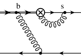
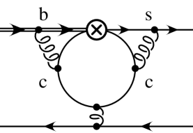
(a)                                                 (b)

Figure 1: Contributions to the $B\to K^{*}\ell^{+}\ell^{-}$ amplitude near the zero recoil point coming from different operators in the OPE Eq. (13). In (a) the circled cross denotes one of the operators ${\cal O}^{(-1,0)}$ of the form $\bar{q}\Gamma iD_{\mu}h_{v}$ or $\bar{q}\Gamma gG_{\mu\nu}h_{v}$, and in (b) it denotes one of the 4-quark operators $(\bar{q}h_{v})(\bar{c}c)$. The contributions in (a) are suppressed relative to the short-distance amplitude by $\Lambda/Q$ (for ${\cal O}^{(-1)}$), $\Lambda^{2}/Q^{2}$ (for ${\cal O}^{(0)}$), and those in (b) by $m_{c}^{4}/Q^{4}$.

Next we include operators whose matrix elements scale like $Q\Lambda$. They are dimension-4 operators of the form $\bar{q}\Gamma iD_{\mu}h_{v}$. A complete set of operators which satisfies the condition (12) and which do not vanish by the equations of motion can be chosen as

$${\cal O}^{(-1)}_{1} = m_{b}\bar{s}_{L}[i\overleftarrow{D}_{\mu}-v_{\mu}(v\cdot i\overleftarrow{D})]h_{vR}$$ (17)

$${\cal O}^{(-1)}_{2} = m_{b}(v\cdot i\partial)\bar{s}_{L}[\gamma_{\mu}-v_{\mu}\mbox{$\not{v}$}]h_{vL}$$ (18)

$${\cal O}^{(-1)}_{3} = m_{b}[i\partial_{\mu}-v_{\mu}(v\cdot i\partial)](\bar{s}_{L}h_{vR})$$ (19)

$${\cal O}^{(-1)}_{4} = m_{b}i\partial_{\nu}(\bar{s}_{L}[\gamma_{\mu}-v_{\mu}\mbox{$\not{v}$}]\gamma^{\nu}h_{vR})$$ (20)

$${\cal O}^{(-1)}_{5} = m_{b}m_{s}\bar{s}_{R}(\gamma_{\mu}-v_{\mu}\mbox{$\not{v}$})h_{vR}\,.$$ (21)

The operator ${\cal O}^{(-1)}_{5}$ describes effects where one chirality flip occurs on the light quark side. Its matrix element scales like $Qm_{s}$.

There are no contributions scaling like $Qm_{c}$, since the dependence on the charm quark mass must contain only even powers of $m_{c}$. The leading contributions containing $m_{c}$ scale like $m_{c}^{2}$ and come from operators similar to (14) and (15). We will define them as

$${\cal O}^{(0)}_{1} = m_{c}^{2}\bar{s}_{L}[\gamma_{\mu}-q_{\mu}\mbox{$\not{q}$}/q^{2}]h_{vL}$$ (22)

$${\cal O}^{(0)}_{2} = im_{b}\frac{m_{c}^{2}}{q^{2}}\bar{s}_{L}\sigma_{\mu\nu}q^{\nu}h_{vR}\,.$$ (23)

There are many operators whose matrix elements scale like $\Lambda^{2}$; generally, they are of the form ${\cal O}^{(0)}_{3,\dots}=\bar{q}\Gamma(iD_{\mu})(iD_{\nu})h_{v}$ or contain one factor of the gluon tensor field strength $\bar{q}\Gamma gG_{\mu\nu}h_{v}$. The latter operators can appear at $O(\alpha_{s}^{0})$ in matching from graphs with $q\bar{q}$ quark loops as shown in Fig. 2(c), and can contribute to the $B\to K^{*}\ell^{+}\ell^{-}$ amplitude through the graph in Fig. 1(a).

Another class of operators appearing in the OPE describes effects of propagating charm quarks (see Fig. 1(b)), and have the form

$${\cal O}^{(2)}=\frac{1}{Q^{2}}(\bar{s}\Gamma h_{v})(\bar{c}\Gamma_{c}iD_{\mu}c)\,.$$ (24)

The explicit form of these operators will be given in the next section, where it is shown that their contributions are further suppressed by $m_{c}^{4}/Q^{4}$ relative to the short-distance amplitude.

To sum up the discussion of this section, we argued that the long-distance effects to $b\to s\ell^{+}\ell^{-}$ decays in the zero recoil region come from well-separated scales satisfying the hierarchy $m_{b}\sim Q>m_{c}>\Lambda$. These effects can be resolved using an OPE as shown in Eq. (13). The contributions of the various operators in the OPE, relative to the dominant short-distance amplitude, are summarized in Table 1, together with the order in matching (in $\alpha_{s}(Q)$) at which they start contributing.

Some of the subleading operators appearing in the OPE give spectator type contributions to the exclusive $B\to K^{*}\ell^{+}\ell^{-}$ amplitude, as shown in Fig. 1. For example, the $O(\Lambda Q)$ operators ${\cal O}_{j}^{(-1)}$ and $O(\Lambda^{2})$ operators ${\cal O}_{j}^{(0)}$ can contribute through the graphs in Fig. 1(a), and the charm operators of the type Eq. (24) contribute as in Fig. 1(b). Such spectator type contributions were studied at lowest order in perturbation theory in LiWi where they were shown to be suppressed at least by $\Lambda/Q$. The effective theory approach used here extends this proof to all orders in $\alpha_{s}$, and shows that the suppression factor is $\alpha_{s}(Q)\Lambda/Q$ (for the contributions from ${\cal O}_{j}^{(-1)}$) and $\Lambda^{2}/Q^{2}$ (for contributions coming from ${\cal O}_{j}^{(0)}$).

We comment briefly on an alternative approach used in Refs. BuMu ; LiWi where the charm quarks and the large scales $\sqrt{q^{2}},m_{b}$ are integrated out simultaneously. Such an approach includes the charm mass effects to all orders in $m_{c}^{2}/m_{b}^{2}$, but has the disadvantage of introducing potentially large power corrections $\sim\Lambda^{2}/m_{c}^{2}$. For this reason we prefer to integrate out only the large scale $Q$ and leave the charm as a dynamical field in the OPE.

The main result of our paper is that the contributions of leading order $O(1)$ and the power suppressed terms $O(m_{c}^{2}/Q^{2})$ to the long-distance amplitude depend only on known form factors and thus can be included without introducing any new hadronic uncertainty. The power suppressed terms of $O(\Lambda/Q)$ can be accounted for in terms of the form factors of the two dimension-4 currents $\bar{q}iD_{\mu}(\gamma_{5})h_{v}$.

Operator	Power counting	Order in matching
${\cal O}_{1,2}^{(-2)}$	1	$\alpha_{s}^{0}(Q)$
${\cal O}_{1-5}^{(-1)}$	$\Lambda/Q$	$\alpha_{s}(Q)$
${\cal O}_{1,2}^{(0)}$	$m_{c}^{2}/Q^{2}$	$\alpha_{s}^{0}(Q)$
${\cal O}_{j>3}^{(0)}$	$\Lambda^{2}/Q^{2}$	$\alpha_{s}^{0}(Q)$
${\cal O}_{i}^{(2)}$	$m_{c}^{4}/Q^{4}$	$\alpha_{s}^{0}(Q)$

Table 1: Contributions to the long-distance amplitude for $b\to s\ell^{+}\ell^{-}$ coming from the different operators in the OPE Eq. (13), together with the order in $\alpha_{s}(Q)$ at which they appear in matching.

In the next Section we compute the matching conditions for these operators at lowest order in perturbation theory.

III Matching

Typical lowest order diagrams contributing to the $T-$products ${\cal T}_{i}^{\mu}(q^{2})$ in QCD are shown in Fig. 1. The matching conditions for the operators appearing in the OPE Eq. (13) are found by computing these graphs and expanding them in powers in $1/Q$. At lowest order in $\alpha_{s}(Q)$ the graph in Fig. 1(a) will match onto ${\cal O}^{(-2)}_{j}$, but not onto the $O(\Lambda Q)$ operators ${\cal O}^{(-1)}_{j}$. These operators appear first at $O(\alpha_{s}(Q))$ from graphs containing one additional gluon as shown in Fig. 1(b).

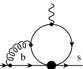
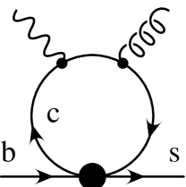
(a)                                             (b)                                             (c)

Figure 2: Graphs in QCD contributing to the matching onto $\bar{s}\Gamma h_{v}$ operators (a), $\bar{s}\Gamma iD_{\mu}h_{v}$ (b) and $\bar{s}gG^{\mu\nu}\Gamma_{\nu}h_{v}$ operators (c). The filled circle denotes the insertion of $Q_{1-6}$. In (c) the wavy line is the virtual photon $\gamma^{*}$ and the curly line denotes a gluon.

An explicit computation of the graph in Fig. 1(a) with one insertion of the operators $Q_{1-6}$ gives the following results for the matrix elements of the $T-$products ${\cal T}_{i}^{\mu}(q^{2})$ on free quark states Heff ; BuMu (we use everywhere naive dimensional regularization (NDR) with an anticommuting $\gamma_{5}$ matrix)

$$\langle{\cal T}_{1}^{\mu}(q^{2})\rangle = \frac{1}{2\pi^{2}}\langle\bar{s}(q^{2}\gamma^{\mu}-q^{\mu}\mbox{$\not{q}$})P_{L}b\rangle\left\{-\frac{2}{3\epsilon}+\frac{2}{3}+4G(m_{c})\right\}$$ (25)

$$\langle{\cal T}_{2}^{\mu}(q^{2})\rangle = \frac{1}{2\pi^{2}}\langle\bar{s}(q^{2}\gamma^{\mu}-q^{\mu}\mbox{$\not{q}$})P_{L}b\rangle\left\{-\frac{2}{9\epsilon}+\frac{2}{9}+\frac{4}{3}G(m_{c})\right\}$$ (26)

$$\langle{\cal T}_{3}^{\mu}(q^{2})\rangle = \frac{1}{2\pi^{2}}\langle\bar{s}(q^{2}\gamma^{\mu}-q^{\mu}\mbox{$\not{q}$})P_{L}b\rangle\left\{-\frac{1}{9\epsilon}-\frac{2}{9}+4G(m_{c})-\frac{2}{3}G(0)-\frac{8}{3}G(m_{b})\right\}$$ (27)

$$\langle{\cal T}_{4}^{\mu}(q^{2})\rangle = \frac{1}{2\pi^{2}}\langle\bar{s}(q^{2}\gamma^{\mu}-q^{\mu}\mbox{$\not{q}$})P_{L}b\rangle\left\{\frac{5}{9\epsilon}-\frac{2}{3}-2G(0)+\frac{4}{3}G(m_{c})-\frac{8}{3}G(m_{b})\right\}$$ (28)

$$\langle{\cal T}_{5}^{\mu}(q^{2})\rangle = \frac{1}{2\pi^{2}}\langle\bar{s}(q^{2}\gamma^{\mu}-q^{\mu}\mbox{$\not{q}$})P_{L}b\rangle\left\{-\frac{1}{3\epsilon}+4G(m_{c})-2G(m_{b})\right\}-\frac{1}{6\pi^{2}}m_{b}\langle\bar{s}(\mbox{$\not{q}$}\gamma_{\mu}-q_{\mu})P_{R}b\rangle$$ (29)

$$\langle{\cal T}_{6}^{\mu}(q^{2})\rangle = \frac{1}{2\pi^{2}}\langle\bar{s}(q^{2}\gamma^{\mu}-q^{\mu}\mbox{$\not{q}$})P_{L}b\rangle\left\{-\frac{1}{9\epsilon}+\frac{4}{3}G(m_{c})-\frac{2}{3}G(m_{b})\right\}-\frac{1}{2\pi^{2}}m_{b}\langle\bar{s}(\mbox{$\not{q}$}\gamma_{\mu}-q_{\mu})P_{R}b\rangle\,.$$ (30)

We denoted here with $G(m_{q})$ the function appearing in the basic fermion loop with mass $m_{q}$

$$G(m_{q})=\int_{0}^{1}\mbox{d}xx(1-x)\log\left(\frac{-q^{2}x(1-x)+m_{q}^{2}-i\epsilon}{\mu^{2}}\right)\,.$$ (31)

In the kinematical region considered here ($4m_{c}^{2}<q^{2}<4m_{b}^{2}$), this function is given explicitly by

$$G(m_{c}) = \frac{1}{6}\log\left(\frac{m_{c}^{2}}{\mu^{2}}\right)-\frac{5}{18}-\frac{2m_{c}^{2}}{3q^{2}}+\frac{1}{6}\sqrt{r}\left(1+\frac{2m_{c}^{2}}{q^{2}}\right)\left(\log\frac{1+\sqrt{r}}{1-\sqrt{r}}-i\pi\right)$$ (32)

$$G(0) = \frac{1}{6}\left[\log\left(\frac{q^{2}}{\mu^{2}}\right)-i\pi\right]-\frac{5}{18}$$ (33)

$$G(m_{b}) = \frac{1}{6}\log\left(\frac{m_{b}^{2}}{\mu^{2}}\right)-\frac{5}{18}-\frac{2m_{b}^{2}}{3q^{2}}+\frac{1}{3}\sqrt{\frac{4m_{b}^{2}}{q^{2}}-1}\left(1+\frac{2m_{b}^{2}}{q^{2}}\right)\arctan\frac{1}{\sqrt{\frac{4m_{b}^{2}}{q^{2}}-1}}$$ (34)

where in $G(m_{c})$ we denoted $r=\sqrt{1-4m_{c}^{2}/q^{2}}$.

To match onto the operators introduced in Sec. II we expand the results (25)-(30) in $1/Q$ and go over to the HQET for the heavy quark field. To the order we work, this amounts to expanding the charm quark loop using

$$G(m_{c})=G(0)-\frac{m_{c}^{2}}{q^{2}}+\left(\frac{m_{c}^{2}}{q^{2}}\right)^{2}\left[\log\left(\frac{q^{2}}{m_{c}^{2}}\right)-i\pi-\frac{1}{2}\right]+\cdots$$ (35)

On the other hand, since we treat $m_{b}^{2}$ and $q^{2}$ as being comparable, the full result for the $b$ quark loop function $G(m_{b})$ has to be kept.

To illustrate the matching computation we show how the result (25) for the T-product containing $Q_{1}$ is reproduced in the operator product expansion (13). Expanding (25) in powers of $m_{c}^{2}/q^{2}$ one finds

$$\langle{\cal T}_{1}^{\mu}\rangle = \frac{1}{2\pi^{2}}[\bar{s}(q^{2}\gamma_{\mu}-q^{\mu}\mbox{$\not{q}$})P_{L}b]\left\{\left[4G(0)+\frac{2}{3}\right]-4\frac{m_{c}^{2}}{q^{2}}\right.$$

$$\left.+4\frac{m_{c}^{4}}{q^{4}}\left[\log\left(\frac{q^{2}}{m_{c}^{2}}\right)-i\pi-\frac{1}{2}\right]+O\left(\frac{m_{c}^{6}}{q^{6}}\right)\right\}$$

The terms of $O(q^{2})$ and $O(m_{c}^{2})$ in this result can be identified with the matrix elements of the operators ${\cal O}_{1}^{(-2)}$ and ${\cal O}_{1}^{(0)}$, respectively, provided that their Wilson coefficients are taken to be

$$C_{1,1}^{(-2)}(\mu) = \frac{1}{2\pi^{2}}\left[4G(0)+\frac{2}{3}\right]\,,\qquad C_{1,1}^{(0)}(\mu)=-\frac{2}{\pi^{2}}$$ (37)

Reproducing the $O(m_{c}^{4}/q^{4})$ term in (III) requires the introduction of dimension-6 operators containing explicit factors of the charm quark field. They are obtained by matching from diagrams where the photon attaches to one of the external quark legs (see Fig. 3). Expanding these graphs in $1/Q$ and keeping only the term of $O(m_{c}/Q^{2})$ gives (the leading term scales like $\sim 1/Q$, but its $b\to s$ matrix element vanishes)

$${\cal T}_{1}^{\mu}(q^{2}) \to{\cal O}^{(2)\mu}=\frac{8Q_{c}}{q^{2}}\left[\bar{c}(\gamma^{\nu}i\overrightarrow{D}^{\mu}-i\overleftarrow{D}^{\mu}\gamma^{\nu})P_{L}c\right](\bar{s}\gamma_{\nu}P_{L}b)$$

$$+\frac{8Q_{c}}{q^{4}}\left[\bar{c}(-\gamma^{\nu}\mbox{$\not{q}$}\gamma^{\mu}(q\cdot i\overrightarrow{D})+\gamma^{\mu}\mbox{$\not{q}$}\gamma^{\nu}(q\cdot i\overleftarrow{D}))P_{L}c\right](\bar{s}\gamma_{\nu}P_{L}b)\,.$$

We dropped here operators which vanish by the equation of motion of the charm quark field $(i\mbox{$\not{D}$}-m_{c})c=0$.

+           $\longrightarrow$      

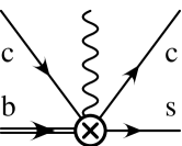
(a)                                     (b)                                     (c)

Figure 3: Graphs contributing to the matching onto operators with explicit charm fields (see, e.g. Eq. (III)). In (a), (b) the filled circle denotes one of the QCD operators $Q_{1-6}$. The crossed circle in (c) denotes the local operator appearing in the OPE with quark content $(\bar{s}b)(\bar{c}c)$. The wavy line is the virtual photon $\gamma^{*}$ connecting to the $e^{+}e^{-}$ lepton pair.

The matrix element of this operator is computed by closing the charm loop, which gives

$$\langle s|{\cal O}^{(2)\mu}|b\rangle=\frac{N_{c}Q_{c}}{\pi^{2}}\langle\bar{s}(q^{2}\gamma^{\mu}-q^{\mu}\mbox{$\not{q}$})P_{L}b\rangle\frac{m_{c}^{4}}{q^{4}}\left\{\frac{1}{\epsilon}+\frac{3}{2}-\log\left(\frac{m_{c}^{2}}{\mu^{2}}\right)\right\}$$ (39)

The coefficient of the logarithmic term $\log m_{c}$ agrees with that in the expansion of the exact result in Eq. (III). This shows that the four-quark operators Eq. (III) reproduce the IR of the full theory result. However, these contributions are suppressed by $m_{c}^{4}/Q^{4}\sim 0.8\%$ relative to those of the leading operators ${\cal O}^{(-2)}_{i}$, so they can be expected to be numerically small. This is fortunate, since their matrix elements on hadronic states would introduce new unknown form factors in addition to those contributing to the short-distance amplitude. In the following we will not include 4-quark operators similar to those in Eq. (III).

Using a similar expansion one finds the matching for all remaining T-products in (25)-(30) onto the operators in the OPE (13). The results for the Wilson coefficients $C_{i,1}^{(-2,0)}$ are

$$\frac{1}{C_{0}^{(v)}(\mu)}C_{1,1}^{(-2)}(\mu) = \frac{1}{2\pi^{2}}\left[4G(0)+\frac{2}{3}\right]-\frac{\alpha_{s}}{(4\pi)^{3}}36C(q^{2})\,,$$ (40)

$$\frac{1}{C_{0}^{(v)}(\mu)}C_{2,1}^{(-2)}(\mu) = \frac{1}{2\pi^{2}}\left[\frac{4}{3}G(0)+\frac{2}{9}\right]-\frac{\alpha_{s}}{(4\pi)^{3}}(-24B(q^{2})+12C(q^{2}))\,,$$ (41)

$$C_{3,1}^{(-2)}(\mu) = \frac{1}{2\pi^{2}}\left[\frac{10}{3}G(0)+\frac{1}{27}-\frac{8}{3}G(m_{b})\right]\,,$$ (42)

$$C_{4,1}^{(-2)}(\mu) = \frac{1}{2\pi^{2}}\left[-\frac{2}{3}G(0)-\frac{7}{9}-\frac{8}{3}G(m_{b})\right]\,,$$ (43)

$$C_{5,1}^{(-2)}(\mu) = \frac{1}{2\pi^{2}}\left[4G(0)-2G(m_{b})-\frac{7}{27}\right]\,,$$ (44)

$$C_{6,1}^{(-2)}(\mu) = \frac{1}{2\pi^{2}}\left[\frac{4}{3}G(0)-\frac{2}{3}G(m_{b})+\frac{1}{9}\right]$$ (45)

and

$$C_{i,1}^{(0)}(\mu) = -\frac{2}{\pi^{2}}\{1\,,\frac{1}{3}\,,1\,,\frac{1}{3}\,,1\,,\frac{1}{3}\}\qquad(i=1-6)$$ (46)

To facilitate the inclusion of the next-to-leading corrections, these results were computed using the operator basis in Ref. CMM , and transformed to the basis in Eq. (7) using 4-dimensional Fierz identities. For this reason, the constant terms in these expressions differ from those in Eqs. (25). With this convention, the Wilson coefficients $C_{i}(\mu)$ used in the remainder of this paper differ beyond the LL approximation from those in Refs. BBL ; BuMu and are equal to the “barred” coefficients $\bar{C}_{i}(\mu)$ defined in Eq. (79) of Ref. BeFeSe . We included here also the next-to-leading results for $C_{1,1}^{(-2)}$ and $C_{2,1}^{(-2)}$, which can be extracted from the recent two-loop computation of Seidel Seidel:2004jh (extending previous approximate results in b2see ). The functions $A(s),B(s),C(s)$ are given in Eqs. (29)-(31) of Seidel:2004jh and can be written as

$$A(q^{2}) = -\frac{104}{243}\log\frac{m_{b}^{2}}{\mu^{2}}+\delta A(q^{2})$$

$$B(q^{2}) = \frac{8}{243}\big{[}\big{(}\frac{4m_{b}^{2}}{q^{2}}-34-17\pi i\big{)}\log\frac{m_{b}^{2}}{\mu^{2}}+8\log^{2}\frac{m_{b}^{2}}{\mu^{2}}+17\log\frac{q^{2}}{m_{b}^{2}}\log\frac{m_{b}^{2}}{\mu^{2}}\big{]}$$

$$- \frac{16}{243}\big{(}1+\frac{2m_{b}^{2}}{q^{2}}\big{)}\sqrt{\frac{4m_{b}^{2}}{q^{2}}-1}\arctan\frac{1}{\sqrt{\frac{4m_{b}^{2}}{q^{2}}-1}}\log\frac{m_{b}^{2}}{\mu^{2}}+\delta B(q^{2})$$

$$C(q^{2}) = -\frac{16}{81}\log\frac{q^{2}}{\mu^{2}}+\frac{428}{243}-\frac{64}{27}\zeta(3)+\frac{16}{81}\pi i$$

The terms $\delta A$ and $\delta B$ do not contain explicit $\mu$ dependence and take the following values at the zero recoil point in $B\to K^{*}e^{+}e^{-}$ (for $\mu=4.8$ GeV and $m_{b}(m_{b})=4.32$ GeV) $\delta A(q^{2}_{\rm max})=0.736+0.836i$, $\delta B(q^{2}_{\rm max})=-1.332+3.058i$. $C_{0}^{(v)}(\mu)$ is one of the Wilson coefficients appearing in the matching of the vector current $\bar{q}\gamma_{\mu}b$ onto HQET currents and is defined in Eq. (51). It accounts for the factorizable two-loop corrections not included in Ref. Seidel:2004jh .

The results for the coefficients $C_{i,2}^{(-2)}(\mu)$ can be computed in a similar way with the results

$$\frac{1}{C_{0}^{(t)}(\mu)}C_{1,2}^{(-2)}(\mu) = 0(\alpha_{s}^{2})\,,\qquad\frac{1}{C_{0}^{(t)}(\mu)}C_{2,2}^{(-2)}(\mu)=-\frac{\alpha_{s}}{(4\pi)^{3}}(48A(q^{2}))\,,$$ (47)

$$C_{i,2}^{(-2)}(\mu) = \frac{1}{\pi^{2}}\{-\frac{2}{9}\,,-\frac{2}{3}\,,\frac{1}{18}\,,\frac{1}{6}\}\qquad(i=3-6)$$

The Wilson coefficient $C_{0}^{(t)}(\mu)$ appears in the matching of the tensor current $\bar{q}i\sigma_{\mu\nu}b$ onto HQET operators and is defined in Eq. (IV). The $O(\alpha_{s}(m_{b})$ terms in the first two coefficients have been extracted from Ref. Seidel:2004jh , where they are given in terms of the function $A(q^{2})$.

The only dimension-4 operators appearing at this order in matching are ${\cal O}_{1,4,5}^{(-1)}$, and are introduced through the matching of the $b$ field onto HQET according to $b=(1+\frac{i\mbox{$\not{D}$}}{2m_{b}})h_{v}$. Their Wilson coefficients are

$$C_{i,1}^{(-1)}(m_{b})=-C_{i,1}^{(-2)}(m_{b})\,,\quad C_{i,4}^{(-1)}(m_{b})=-C_{i,5}^{(-1)}(m_{b})=\frac{1}{2}C_{i,1}^{(-2)}(m_{b})\qquad(i=1-6)\,.$$ (48)

At two-loop order in the matching, all the other dimension-4 operators will appear, through the dependence of graphs such as those in Fig. 2(b) on external quark momenta.

The gluonic penguin $Q_{8}$ contributes to the long-distance amplitude at leading order in $1/Q$ through one-loop graphs. The corresponding one-loop graphs were computed in the second reference of b2see in an expansion in $q^{2}/m_{b}^{2}$ and in Ref. BeFeSe for arbitrary $q^{2}$. Its contributions to the Wilson coefficients of the leading operators are

$$C_{8,1}^{(-2)}(\mu)=\frac{\alpha_{s}}{16\pi^{3}}F_{8}^{(9)}(q^{2})\,,\qquad C_{8,2}^{(-2)}(\mu)=-\frac{\alpha_{s}}{8\pi^{3}}F_{8}^{(7)}(q^{2})$$ (49)

with $F_{8}^{(9,7)}(q^{2})$ given in Eqs. (82), (83) of Ref. BeFeSe . The operator $Q_{8}$ contributes also at tree level through gluon-photon scattering graphs (with the photon coupling to the $b$ and $s$ quarks). Expanding these graphs in powers of $1/Q$ one finds at leading order

$${\cal T}^{\mu}_{8}\to-\frac{m_{b}Q_{b}}{(4\pi)^{2}v\cdot q}\bar{s}_{L}\sigma_{\alpha\beta}gG^{\alpha\beta}\gamma^{\mu}h_{vR}+\frac{Q_{s}}{8\pi^{2}}\bar{s}_{L}\gamma_{\mu}\mbox{$\not{v}$}\sigma_{\alpha\beta}gG^{\alpha\beta}h_{vR}\,.$$ (50)

The matrix elements of these dimension-6 operators are suppressed by $\Lambda^{2}/Q^{2}$.

The one-loop graphs in Fig. 2(c) with one insertion of $Q_{1-6}$ produce dimension-5 operators containing the gluon field tensor of the form $\bar{s}gG_{\mu\nu}h_{v}$. Although their Wilson coefficients start at $O(\alpha_{s}^{0})$, their matrix elements are $\sim\Lambda^{2}$, and therefore are suppressed by $\Lambda^{2}/Q^{2}$ relative to the short distance amplitude. We will neglect all these higher dimensional operators and keep only the $O(1),O(m_{c}^{2}/m_{b}^{2})$ and $O(\Lambda/m_{b})$ terms in the long distance amplitude.

IV Matrix elements

In this section we use the OPE result Eq. (13) for the long-distance amplitudes ${\cal T}_{i}(q^{2})$ to compute the hadronic amplitude $A_{\mu}^{(V)}$ in Eq. (II) up to and including corrections of order $O(\alpha_{s}(Q),\Lambda/m_{b},m_{c}^{2}/m_{b}^{2})$. At this point we encounter a technical complication connected with the fact that the OPE was performed in terms of HQET operators, while the matrix elements of the QCD currents $\bar{s}\Gamma b$ appearing in the factorizable matrix elements of $Q_{7,9}$ are expressed in terms of physical form factors. This means that the matrix elements of the operators ${\cal O}^{(-2)}_{1,2}$ are given in terms of HQET form factors, which are not known. Also, keeping all $O(\Lambda/m_{b})$ contributions requires that we include also $T$-products of the ${\cal O}^{(-2)}_{1,2}$ operators with $1/m_{b}$ sub-leading terms in the HQET Lagrangian. Such nonlocal matrix elements introduce additional unknown form factors. This proliferation of unknown matrix elements appears to preclude a simple form for our final result.

We will show next that it is possible to absorb all these nonlocal matrix elements into the physical form factors, through a simple reorganization of the operator expansion, such that one is left only with local $1/m_{b}$ corrections. This can be achieved by expressing the leading operators ${\cal O}^{(-2)}_{i}$ in terms of QCD operators, up to dimension-4 HQET operators $\bar{s}iD_{\mu}(\gamma_{5})h_{v}$. Technically, this is obtained by inverting the HQET matching relations (we assume here everywhere the NDR scheme)

$$\bar{s}_{L}\gamma_{\mu}b_{L} = C_{0}^{(v)}(\mu)\bar{s}_{L}\gamma_{\mu}h_{vL}+C_{1}^{(v)}(\mu)\bar{s}_{L}v_{\mu}h_{vR}+\frac{1}{2m_{b}}\bar{s}_{L}\gamma_{\mu}i\mbox{$\not{D}$}h_{vR}+O(1/m_{b}^{2})$$ (51)

$$\bar{s}_{L}i\sigma_{\mu\nu}q^{\nu}b_{R} = C_{0}^{(t)}(\mu)\bar{s}_{L}i\sigma_{\mu\nu}q^{\nu}h_{vR}+C_{1}^{(t)}(\mu)\bar{s}_{L}[(v\cdot q)\gamma_{\mu}-\mbox{$\not{q}$}v_{\mu}]h_{vL}$$

$$+\frac{1}{2m_{b}}\bar{s}_{L}i\sigma_{\mu\nu}q^{\nu}i\mbox{$\not{D}$}h_{vL}+O(1/m_{b}^{2})\,.$$

The Wilson coefficients $C_{i}^{(v,t)}(\mu)$ are given at one-loop by EiHi

$$C_{0}^{(v)}(\mu) = 1-\frac{\alpha_{s}C_{F}}{4\pi}(3\log\frac{\mu}{m_{b}}+4)\,,\qquad C_{1}^{(v)}(\mu)=\frac{\alpha_{s}C_{F}}{2\pi}$$ (53)

$$C_{0}^{(t)}(\mu) = 1-\frac{\alpha_{s}C_{F}}{4\pi}(5\log\frac{\mu}{m_{b}}+4)\,,\qquad C_{1}^{(t)}=O(\alpha^{2}_{s})\,.$$ (54)

In the $O(1/m_{b})$ terms we work at tree level in the matching, which will be sufficient for the precision required here, although the method can be extended to any order in $\alpha_{s}(m_{b})$.

Solving the matching relations Eqs. (51), (IV) for the leading order HQET operators appearing in the OPE ${\cal O}_{1,2}^{(-2)}$ one finds

$$\bar{s}_{L}(q^{2}\gamma_{\mu}-\mbox{$\not{q}$}q_{\mu})h_{vL} = \frac{1}{C_{0}^{(v)}(\mu)}\bar{s}_{L}(q^{2}\gamma_{\mu}-\mbox{$\not{q}$}q_{\mu})b_{L}+{\cal O}_{1}^{(-1)}-\frac{1}{2}{\cal O}_{4}^{(-1)}+\frac{1}{2}{\cal O}_{5}^{(-1)}$$ (55)

$$\bar{s}_{L}i\sigma^{\mu\nu}q_{\nu}h_{vR} = \frac{1}{C_{0}^{(t)}(\mu)}\bar{s}_{L}i\sigma^{\mu\nu}q_{\nu}b_{R}-\frac{C_{1}^{(t)}(\mu)}{C_{0}^{(v)}(\mu)C_{0}^{(t)}(\mu)}\bar{s}_{L}[(v\cdot q)\gamma_{\mu}-v_{\mu}\mbox{$\not{q}$}]b_{L}$$ (56)

We neglected here terms of $O(\alpha_{s}(m_{b})\Lambda/m_{b})$.

Substituting these results into the OPE, the leading terms can be written in terms of physical $B\to K^{*}$ form factors, with corrections of $O(\Lambda/m_{b})$ coming from local dimension-4 operators ${\cal O}_{1-5}^{(-1)}$

$$A_{\mu}^{(V)} = -C_{7}^{\rm eff}(\mu)\frac{2m_{b}}{q^{2}}\langle\bar{s}i\sigma_{\mu\nu}q^{\nu}(1+\gamma_{5})b\rangle$$

$$+C_{9}^{\rm eff}(\mu)\langle\bar{s}\gamma_{\mu}(1-\gamma_{5})b\rangle+\frac{1}{q^{2}}\sum_{i=1}^{5}B_{i}(\mu)\langle{\cal O}_{i}^{(-1)}\rangle\,.$$

We absorbed here the contributions from the leading terms in Eqs. (55), (56) into a redefinition of the Wilson coefficients $C_{7,9}$

$$C_{7}(\mu) \to C_{7}^{\rm eff}(\mu)=C_{7}(\mu)+2\pi^{2}\sum_{i=1}^{6,8}C_{i}(\mu)\left[\frac{C_{i,2}^{(-2)}(\mu)}{C_{0}^{(t)}(\mu)}+C_{i,2}^{(0)}(\mu)\frac{m_{c}^{2}}{q^{2}}\right]$$ (58)

$$C_{9}(\mu) \to C_{9}^{\rm eff}(\mu)=C_{9}(\mu)$$

$$-4\pi^{2}\sum_{i=1}^{6,8}C_{i}(\mu)\left[\frac{C_{i,1}^{(-2)}(\mu)}{C_{0}^{(v)}(\mu)}-\frac{C_{i,2}^{(-2)}(\mu)}{C_{0}^{(t)}(\mu)C_{0}^{(v)}(\mu)}C_{1}^{(t)}(\mu)+C_{i,1}^{(0)}(\mu)\frac{m_{c}^{2}}{q^{2}}\right]\,.$$

The $O(1)$ and $O(m_{c}^{2}/q^{2})$ contributions to the long-distance amplitude are contained in $C_{7,9}^{\rm eff}$, and the $O(\Lambda/m_{b})$ part is encoded in the matrix elements of ${\cal O}_{i}^{(-1)}$. Note that the effective Wilson coefficients $C_{7,9}^{\rm eff}$ introduced here are different from the “effective Wilson coefficients” commonly used in the literature $\tilde{C}_{7,9}^{\rm eff}$ BuMu ; b2see . The latter include contributions from the matrix elements of the operators $Q_{1-9}$ (usually computed in perturbation theory), and are thus dependent on the final state. In contrast, our effective Wilson coefficients are state independent, and encode only contributions from the hard scale $\mu\sim m_{b}$.

Combining everything, the next-to-leading expressions for the effective Wilson coefficients are

$$C_{9}^{\rm eff} = C_{9}-(C_{1}+\frac{C_{2}}{3})[8G(0)+\frac{4}{3}]-C_{3}[\frac{20}{3}G(0)-\frac{16}{3}G(m_{b})+\frac{2}{27}]+C_{4}[\frac{4}{3}G(0)+\frac{16}{3}G(m_{b})+\frac{14}{9}]$$

$$- C_{5}[8G(0)-4G(m_{b})-\frac{14}{27}]-C_{6}[\frac{8}{3}G(0)-\frac{4}{3}G(m_{b})+\frac{2}{9}]+\frac{\alpha_{s}}{4\pi}[C_{1}9C(q^{2})+C_{2}(-6B(q^{2})+3C(q^{2}))-C_{8}F_{8}^{(9)}(q^{2})]$$

$$C_{7}^{\rm eff} = C_{7}-\frac{4}{9}C_{3}-\frac{4}{3}C_{4}+\frac{1}{9}C_{5}+\frac{1}{3}C_{6}+\frac{\alpha_{s}}{4\pi}[-C_{2}6A(q^{2})-C_{8}F_{8}^{(7)}(q^{2})]$$ (61)

The effective Wilson coefficient $C_{9}^{\rm eff}$ is RG invariant. At the order we work here, it satisfies the RG equation

$$\mu\frac{d}{d\mu}C_{9}^{\rm eff}(\mu)=O(\alpha_{s}^{2}C_{1,2},\alpha_{s}C_{3-6})\,.$$ (62)

The coefficient $C_{7}^{\rm eff}(\mu)$ satisfies a RG equation

$$\mu\frac{\rm d}{{\rm d}\mu}C_{7}^{\rm eff}(\mu)=\gamma_{7}(\alpha_{s})C_{7}^{\rm eff}(\mu)$$ (63)

with anomalous dimension $\gamma_{7}(\alpha_{s})=\gamma_{t}(\alpha_{s})-\gamma_{m}(\alpha_{s})$ (see Eqs. (138) and (139) for definitions).

The Wilson coefficients of the dimension-4 operators $B_{i}(\mu)$ are given by

$$B_{1}(\mu) = 8\pi^{2}\sum_{i}C_{i}(\mu)(C_{i,1}^{(-1)}(\mu)+C_{i,1}^{(-2)}(\mu))$$ (64)

$$B_{2}(\mu) = 8\pi^{2}\sum_{i}C_{i}(\mu)C_{i,2}^{(-1)}(\mu)$$ (65)

$$B_{3}(\mu) = 8\pi^{2}\sum_{i}C_{i}(\mu)C_{i,3}^{(-1)}(\mu)$$ (66)

$$B_{4}(\mu) = 8\pi^{2}\sum_{i}C_{i}(\mu)(C_{i,4}^{(-1)}(\mu)-\frac{1}{2}C_{i,1}^{(-2)}(\mu))$$ (67)

$$B_{5}(\mu) = 8\pi^{2}\sum_{i}C_{i}(\mu)(C_{i,5}^{(-1)}(\mu)+\frac{1}{2}C_{i,1}^{(-2)}(\mu))\,.$$ (68)

These Wilson coefficients start at $O(\alpha_{s})$ in matching. By absorbing the factor of $8\pi^{2}$ in their definition, their expansion in $\alpha_{s}(Q)$ starts with a term of order $\alpha_{s}(Q)/\pi$. At the order we work (keeping terms in the OPE of $O(\alpha_{s},\Lambda/Q,m_{c}^{2}/Q^{2})$, but neglecting $O(\alpha_{s}\Lambda/Q)$ terms), they all vanish $B_{1-5}=0$. However, we will include them in the following expressions, which is required for a complete result to $O(\Lambda/m_{b})$ accuracy for the long-distance amplitude.

It is convenient to parameterize the physical amplitudes $A_{\mu}^{(V,A)}$ introduced in Eq. (8) in terms of eight scalar form factors ${\cal A}^{(V,A)}-{\cal D}^{(V,A)}$ defined as

$$A_{\mu}^{(V,A)} = {\cal A}^{(V,A)}(q^{2})i\varepsilon_{\mu\nu\lambda\sigma}\eta^{*\nu}(p+k)^{\lambda}(p-k)^{\sigma}+{\cal B}^{(V,A)}(q^{2})\eta_{\mu}^{*}$$

$$+{\cal C}^{(V,A)}(q^{2})(\eta^{*}\cdot p)(p+k)_{\mu}+{\cal D}^{(V,A)}(q^{2})(\eta^{*}\cdot p)(p-k)_{\mu}$$

The $B\to K^{*}e^{+}e^{-}$ decay rate can be represented as a sum over the helicity $\lambda=\pm 1,0$ of the vector meson. In the limit of massless leptons, this is given by

$$\frac{d\Gamma(B\to K^{*}e^{+}e^{-})}{dq^{2}}=\frac{4G_{F}^{2}|V_{tb}V_{ts}^{*}|^{2}\alpha^{2}}{3m_{B}^{2}(4\pi)^{5}}q^{2}|\vec{q}\,|\sum_{\lambda=\pm 1,0}\left\{|H_{\lambda}^{(V)}|^{2}+|H_{\lambda}^{(A)}|^{2}\right\}$$ (70)

where the $H_{\lambda}^{(V)}$ and $H_{\lambda}^{(A)}$ correspond to the vector and axial leptons coupling, respectively. Expressed in terms of the scalar amplitudes ${\cal A,B,C}$ introduced in Eq. (IV), they are given by ($i=V,A$)

$$H_{\pm}^{(i)}(q^{2}) = \mp 2m_{B}|\vec{q}|{\cal A}^{(i)}(q^{2})-{\cal B}^{(i)}(q^{2})$$ (71)

$$H_{0}^{(i)}(q^{2}) = \frac{1}{2m_{V}\sqrt{q^{2}}}\left\{(-q^{2}+m_{B}^{2}-m_{V}^{2}){\cal B}^{(i)}(q^{2})+4m_{B}^{2}\vec{q}\,^{2}{\cal C}^{(i)}(q^{2})\right\}\,.$$ (72)

The explicit results for the amplitudes ${\cal A}^{(V,A)}-{\cal D}^{(V,A)}$ are obtained by taking matrix elements on physical states and are given by

$${\cal A}^{(V)}(q^{2}) = -C_{7}^{\rm eff}(\mu)\frac{2m_{b}}{q^{2}}g_{+}(q^{2})+C_{9}^{\rm eff}(\mu)g(q^{2})+{\cal A}_{\rm l.d.}(q^{2})$$ (73)

$${\cal B}^{(V)}(q^{2}) = -C_{7}^{\rm eff}(\mu)\frac{2m_{b}}{q^{2}}[(m_{B}^{2}-m_{V}^{2})g_{+}(q^{2})+q^{2}g_{-}(q^{2})]-C_{9}^{\rm eff}(\mu)f(q^{2})+{\cal B}_{\rm l.d.}(q^{2})$$ (74)

$${\cal C}^{(V)}(q^{2}) = -C_{7}^{\rm eff}(\mu)\frac{2m_{b}}{q^{2}}[-g_{+}(q^{2})+q^{2}h(q^{2})]-C_{9}^{\rm eff}(\mu)a_{+}(q^{2})+{\cal C}_{\rm l.d.}(q^{2})$$ (75)

$${\cal D}^{(V)}(q^{2}) = C_{7}^{\rm eff}(\mu)\frac{2m_{b}}{q^{2}}[g_{-}(q^{2})+(m_{B}^{2}-m_{V}^{2})h(q^{2})]-C_{9}^{\rm eff}(\mu)a_{-}(q^{2})+{\cal D}_{\rm l.d.}(q^{2})$$ (76)

and

$${\cal A}^{(A)}(q^{2}) = C_{10}g(q^{2})$$ (77)

$${\cal B}^{(A)}(q^{2}) = -C_{10}f(q^{2})$$ (78)

$${\cal C}^{(A)}(q^{2}) = -C_{10}a_{+}(q^{2})$$ (79)

$${\cal D}^{(A)}(q^{2}) = -C_{10}a_{-}(q^{2})\,.$$ (80)

The coefficients ${\cal D}^{(V,A)}(q^{2})$ do not contribute to the $B\to Ve^{+}e^{-}$ decay rate into massless leptons, but are relevant for the $B\to V\tau^{+}\tau^{-}$ mode. We will not consider them further. The $O(\Lambda/Q)$ contribution to the long-distance contribution appears as matrix elements of the local dimension-4 operators ${\cal O}_{i}^{(-1)}$ (denoted as ${\cal A}_{\rm l.d.}(q^{2})-{\cal D}_{\rm l.d.}(q^{2})$ in Eqs. (73)-(76)). They are given explicitly by

$${\cal A}_{\rm l.d.}(q^{2}) = \frac{1}{2m_{b}}d^{(0)}(q^{2})B_{1}+\frac{1}{2m_{b}}(\bar{\Lambda}-v.k)g(q^{2})B_{2}-\frac{1}{4m_{b}}[(1+\frac{\bar{\Lambda}}{m_{B}})g_{+}(q^{2})+(1-\frac{\bar{\Lambda}}{m_{B}})g_{-}(q^{2})]B_{4}$$

$$+\frac{m_{s}}{2m_{b}}g(q^{2})B_{5}$$

$${\cal B}_{\rm l.d.}(q^{2}) = \frac{1}{2m_{b}}d_{1}^{(0)}(q^{2})B_{1}-\frac{1}{2m_{b}}(\bar{\Lambda}-v.k)f(q^{2})B_{2}$$

$$-\frac{1}{2m_{b}}[(\bar{\Lambda}v-k).(p+k)g_{+}(q^{2})+(\bar{\Lambda}v-k).(p-k)g_{-}(q^{2})]B_{4}+\frac{m_{s}}{2m_{b}}f(q^{2})B_{5}$$

$${\cal C}_{\rm l.d.}(q^{2}) = \frac{1}{2m_{b}}[d_{+}^{(0)}(q^{2})-\frac{\bar{\Lambda}-v.k}{2m_{b}}s(q^{2})]B_{1}-\frac{1}{2m_{b}}(\bar{\Lambda}-v.k)[a_{+}(q^{2})+\frac{1}{2m_{b}}s(q^{2})]B_{2}$$

$$-\frac{1}{4m_{b}}(1-\frac{v.k}{m_{B}})s(q^{2})B_{3}+(\frac{\bar{\Lambda}}{2m_{b}^{2}}g_{+}(q^{2})-\frac{1}{2}(\bar{\Lambda}-v.k)h(q^{2})-\frac{1}{4m_{b}}s(q^{2}))B_{4}$$

$$+\frac{m_{s}}{2m_{b}}[a_{+}(q^{2})+\frac{1}{2m_{b}}s(q^{2})]B_{5}$$

The form factors appearing here are defined in the Appendix. The corresponding result for ${\cal D}_{\rm l.d.}(q^{2})$ can be obtained from the Ward identity which gives ${\cal B}_{\rm l.d.}(q^{2})+(m_{B}^{2}-m_{V}^{2}){\cal C}_{\rm l.d.}(q^{2})+q^{2}{\cal D}_{\rm l.d.}(q^{2})=0$. Expanding in powers of $1/m_{b}$ and keeping the leading terms gives ${\cal D}_{\rm l.d.}(q^{2})=-{\cal C}_{\rm l.d.}(q^{2})+O(\Lambda/m_{b})$.

For completeness we quote here also the relevant results for the semileptonic decay $B\to\rho e\bar{\nu}$. The decay rate is given by a sum over contributions corresponding to helicities of the final vector meson $\lambda=\pm,0$

$$\frac{d\Gamma(\bar{B}\to\rho e\nu)}{dq^{2}}=\frac{G_{F}^{2}|V_{ub}|^{2}}{96\pi^{3}m_{B}^{2}}q^{2}|\vec{q}\,|\sum_{\lambda=\pm 1,0}|H_{\lambda}|^{2}$$ (84)

where the helicity amplitudes are given by

$$H_{\pm}(q^{2}) = \mp 2m_{B}|\vec{q}|g(q^{2})+f(q^{2})$$ (85)

$$H_{0}(q^{2}) = \frac{1}{2m_{V}\sqrt{q^{2}}}\left\{(q^{2}-m_{B}^{2}+m_{V}^{2})f(q^{2})-4m_{B}^{2}\vec{q}\,^{2}a_{+}(q^{2})\right\}\,.$$ (86)

V Phenomenology

In the low recoil region, the amplitudes ${\cal A}^{(V)},{\cal B}^{(V)},{\cal C}^{(V)}$ for $B\to K^{*}\ell^{+}\ell^{-}$ are dominated by the operator $Q_{9}$. The contribution proportional to $C_{7}$ can be expressed in terms of the $C_{9}$ terms using the form factor relations Eqs. (129),(144),(145) given in the Appendix. Keeping terms to subleading order in $\Lambda/m_{b}$, these amplitudes can be written as

$${\cal A}^{(V)}(q^{2}) = C_{9}^{\rm eff}g(q^{2})\left\{1+\frac{C_{7}^{\rm eff}}{C_{9}^{\rm eff}}\frac{2m_{b}}{q^{2}}\left[(1+\frac{2D_{0}^{(v)}(\mu)}{C_{0}^{(v)}(\mu)})m_{b}+m_{q}+2\frac{d^{(0)}(q^{2})}{g(q^{2})}\right]+\frac{{\cal A}_{\rm l.d.}(q^{2})}{C_{9}^{\rm eff}g(q^{2})}+O(\frac{\Lambda^{2}}{m_{b}^{2}})\right\}$$ (87)

$${\cal B}^{(V)}(q^{2}) = -C_{9}^{\rm eff}f(q^{2})\left\{1+\frac{C_{7}^{\rm eff}}{C_{9}^{\rm eff}}\frac{2m_{b}}{q^{2}}\left[(1+\frac{2D_{0}^{(v)}(\mu)}{C_{0}^{(v)}(\mu)})m_{b}-m_{q}-2\frac{d_{1}^{(0)}(q^{2})}{f(q^{2})}\right]-\frac{{\cal B}_{\rm l.d.}(q^{2})}{C_{9}^{\rm eff}f(q^{2})}+O(\frac{\Lambda^{2}}{m_{b}^{2}})\right\}$$ (88)

$${\cal C}^{(V)}(q^{2}) = -C_{9}^{\rm eff}a_{+}(q^{2})\left\{1+\frac{C_{7}^{\rm eff}}{C_{9}^{\rm eff}}\frac{2m_{b}}{q^{2}}\left[(1+\frac{2D_{0}^{(v)}(\mu)}{C_{0}^{(v)}(\mu)})m_{b}-m_{q}-2\frac{d_{+}^{(0)}(q^{2})}{a_{+}(q^{2})}\right]+\frac{{\cal C}_{\rm l.d.}(q^{2})}{C_{9}^{\rm eff}a_{+}(q^{2})}+O(\frac{\Lambda^{2}}{m_{b}^{2}})\right\}\,.$$ (89)

Inserting these results into the expressions for the helicity amplitudes $H_{\lambda}^{(V)}(q^{2})$ one finds

$$H_{\pm}^{(V)}(q^{2}) = \mp 2m_{B}m_{V}\sqrt{y^{2}-1}C_{9}^{\rm eff}g(q^{2})(1+\delta+r_{a})+C_{9}^{\rm eff}f(q^{2})(1+\delta+r_{b})$$ (90)

$$H_{0}^{(V)}(q^{2}) = -\frac{m_{B}y-m_{V}}{\sqrt{q^{2}}}C_{9}^{\rm eff}f(q^{2})(1+\delta+r_{b})-2m_{B}^{2}m_{V}\frac{y^{2}-1}{\sqrt{q^{2}}}C_{9}^{\rm eff}a_{+}(q^{2})(1+\delta+r_{c})$$ (91)

Here $1+\delta(q^{2})$ scales like $m_{b}^{0}$ and $r_{a,b,c}(q^{2})$ parameterize the $1/m_{b}$ correction. Their explicit expressions are

$$\delta(q^{2}) = \frac{C_{7}^{\rm eff}(\mu)}{C_{9}^{\rm eff}}\frac{2m_{b}^{2}(\mu)}{q^{2}}\left(1+\frac{2D_{0}^{(v)}(\mu)}{C_{0}^{(v)}(\mu)}\right)$$ (92)

$$r_{a}(q^{2}) = \delta(q^{2})\frac{1}{m_{b}}(m_{q}+2\frac{d^{(0)}(q^{2})}{g(q^{2})})+\frac{{\cal A}_{\rm l.d.}(q^{2})}{C_{9}^{\rm eff}g(q^{2})}$$ (93)

$$r_{b}(q^{2}) = \delta(q^{2})\frac{1}{m_{b}}(-m_{q}-2\frac{d_{1}^{(0)}(q^{2})}{f(q^{2})})+\frac{{\cal B}_{\rm l.d.}(q^{2})}{C_{9}^{\rm eff}f(q^{2})}$$ (94)

$$r_{c}(q^{2}) = \delta(q^{2})\frac{1}{m_{b}}(-m_{q}-2\frac{d_{+}^{(0)}(q^{2})}{a_{+}(q^{2})})-\frac{{\cal C}_{\rm l.d.}(q^{2})}{C_{9}^{\rm eff}a_{+}(q^{2})}\,.$$ (95)

Combining the RG equations satisfied by $C_{7}^{\rm eff}(\mu)$ Eq. (63) and by the $1+2D_{0}^{(v)}(\mu)/C_{0}^{(v)}(\mu)$ factor Eq. (137), one can see that the $\delta(q^{2})$ parameter is RG invariant.

These results imply that the $H_{\lambda}^{(V)}(q^{2})$ amplitudes for rare $B\to V\ell^{+}\ell^{-}$ decays are related at leading order in $\Lambda/m_{b}$ to those for semileptonic decay $B\to Ve\bar{\nu}$ with a common proportionality factor

$$H_{\lambda}^{(V)}(q^{2})=C_{9}^{\rm eff}(1+\delta(q^{2})+O(\Lambda/m_{b}))H_{\lambda}(q^{2})\,.$$ (96)

Combining this with the rate formulas one finds a relation among the decay rates for the rare and semileptonic decays

$$\frac{\mbox{d}\Gamma(\bar{B}\to\rho e\nu)/\mbox{d}q^{2}}{\mbox{d}\Gamma(\bar{B}\to K^{*}\ell^{+}\ell^{-})/\mbox{d}q^{2}}=\frac{|V_{ub}|^{2}}{|V_{tb}V_{ts}^{*}|^{2}}\cdot\frac{8\pi^{2}}{\alpha^{2}}\cdot\frac{1}{|C_{9}^{\rm eff}(1+\delta(q^{2}))|^{2}+|C_{10}|^{2}}\frac{\sum_{\lambda}|H_{\lambda}^{B\to\rho}(q^{2})|^{2}}{\sum_{\lambda}|H_{\lambda}^{B\to K^{*}}(q^{2})|^{2}}$$ (97)

The corrections to this relation are of order $O(\Lambda/m_{b})$ and can be expressed in terms of the three parameters $r_{a,b,c}(q^{2})$ introduced above.

The ratio of decay rates in Eq. (97) has been considered previously in Ref. SaYa ; LiWi ; LSW in connection with a method for determining $|V_{ub}|$. This requires some information about the SU(3) breaking ratio of helicity amplitudes appearing on the right-hand side

$$R_{B}(y)\equiv\frac{\sum_{\lambda}|H_{\lambda}^{B\to\rho}(y)|^{2}}{\sum_{\lambda}|H_{\lambda}^{B\to K^{*}}(y)|^{2}}$$ (98)

It has been proposed in LiWi ; LSW to determine $R_{B}$ in terms of the corresponding ratio of $D\to\rho/K^{*}$ decay amplitudes $R_{D}(y)$ using a double ratio Grin , up to corrections linear in both heavy quark and SU(3) symmetry breaking

$$R_{B}(y)=R_{D}(y)(1+O(m_{s}(\frac{1}{m_{c}}-\frac{1}{m_{b}}))$$ (99)

In this relation, the two sides must be taken at the same value of the kinematical variable $y=E_{V}/m_{V}$. A chiral perturbation theory computation LSW at the zero recoil point $y=1$ shows that the corrections to this prediction are even smaller than suggested by the naive dimensional estimate Eq. (99). We do not have anything new to add on this point, and focus instead on the structure of the denominator in Eq. (97).

The results of our paper improve on previous work in two main respects. First, we point out that the rate ratio (97) can be computed at leading order in $1/m_{b}$ over the entire small recoil region, and not only at the zero recoil point $q^{2}=(m_{B}-m_{V})^{2}$. This has important experimental implications, as the rate itself vanishes at the zero recoil point, such that measuring the ratio in Eq. (97) would involve an extrapolation from $q^{2}<q^{2}_{\rm max}$. Most importantly, Eq. (97) allows the determination of $V_{ub}$ using ratios of rates integrated over a range in $q^{2}$, as long as such a range is still contained within the low recoil region.

Second, we present explicit results for the subleading $O(\Lambda/m_{b})$ correction to this result in terms of new form factors contained in the parameters $r_{a,b,c}(q^{2})$. Using model computations of these form factors, this allows a quantitative estimate of the power corrections effect on the $V_{ub}$ determination.

In the rest of this section we will study in some detail the (RG-invariant) quantity $N_{\rm eff}(q^{2})$ defined through the ratio of rare radiative and semileptonic decays in Eq. (97)

$$\frac{\mbox{d}\Gamma(\bar{B}\to\rho e\nu)/\mbox{d}q^{2}}{\mbox{d}\Gamma(\bar{B}\to K^{*}\ell^{+}\ell^{-})/\mbox{d}q^{2}}=\frac{|V_{ub}|^{2}}{|V_{tb}V_{ts}^{*}|^{2}}\cdot\frac{8\pi^{2}}{\alpha^{2}}\cdot\frac{1}{N_{\rm eff}(q^{2})}\frac{\sum_{\lambda}|H_{\lambda}^{B\to\rho}(q^{2})|^{2}}{\sum_{\lambda}|H_{\lambda}^{B\to K^{*}}(q^{2})|^{2}}$$ (100)

The results of this paper offer a systematic way of computing this quantity in an expansion in $\alpha_{s}(Q)$, $m_{c}^{2}/Q^{2}$ and $\Lambda/m_{b}$. The precision of a $|V_{ub}|$ determination using this method is ultimately determined by the precision in our knowledge of this parameter. There are several sources of uncertainty in $N_{\rm eff}(q^{2})$, coming from scale dependence, $O(\Lambda/m_{b})$ power corrections and duality violations. We will consider them in turn.

At leading order in $\Lambda/m_{b}$, the $N_{\rm eff}(q^{2})$ parameter is given by

$$N_{\rm eff}(q^{2})=|C_{9}^{\rm eff}+\frac{2m_{b}(\mu)^{2}}{q^{2}}C_{7}^{\rm eff}\left(1+2\frac{D_{0}^{(v)}(\mu)}{C_{0}^{(v)}(\mu)}\right)|^{2}+|C_{10}|^{2}+O(\Lambda/m_{b})\,.$$ (101)

We give in Table II results for the effective Wilson coefficients $C_{7,9}^{\rm eff}$ at several values of the renormalization scale $\mu\sim m_{b}$. We work both at leading log order (next-to-leading log order for $C_{9}(\mu)$), and at next-to-leading order (NNLL order for $C_{9}$). In each of these approximations the combination of effective Wilson coefficients in Eq. (101) satisfies the RG equation

$$\mu\frac{d}{d\mu}\left[C_{9}^{\rm eff}+\frac{2m_{b}(\mu)^{2}}{q^{2}}C_{7}^{\rm eff}\left(1+2\frac{D_{0}^{(v)}(\mu)}{C_{0}^{(v)}(\mu)}\right)\right]=\left\{\begin{array}[]{cc}O(\alpha_{s})\,,&\mbox{(LL)}\\ O(\alpha_{s}^{2}C_{1,2},\alpha_{s}C_{3-6})\,,&\mbox{(NLL)}\\ \end{array}\right.$$ (104)

The structure of the NNLL running for the Wilson coefficients in the $b\to se^{+}e^{-}$ weak Hamiltonian was given in Ref. BoMiUr (see also BeFeSe ). The complete NNLL result requires the 3-loop mixing of the four-quark operators into $Q_{7,9}$, which was obtained only recently ADM . We use here the full NNLL results for the Wilson coefficients $C_{7,9}$, which were presented in BoGaGoHa . The factor containing $D_{0}^{(v)}(\mu)$ can be extracted from Eq. (130) and its inclusion is necessary at NLL to achieve the scale independence of $N_{\rm eff}$ to this order.

	$\mu_{b}$ (GeV)	$C_{9}$	$C_{7}$	$C_{9}^{\rm eff}(y=1)$	$C_{9}^{\rm eff}(y=1.5)$	$C_{7}^{\rm eff}(y=1)$	$C_{7}^{\rm eff}(y=1.5)$	$N_{\rm eff}(y=1)$	$N_{\rm eff}(y=1.5)$
	2.4	4.378	-0.388	$4.315+0.198i$	$4.338+0.198i$	$C_{7}$	$C_{7}$	30.80	28.96
LL	4.8	4.140	-0.343	$4.331+0.550i$	$4.395+0.550i$	$C_{7}$	$C_{7}$	33.37	32.34
	9.6	3.760	-0.304	$4.420+0.822i$	$4.513+0.822i$	$C_{7}$	$C_{7}$	35.81	35.38
	2.4	4.510	-0.366	$4.685+0.494i$	$4.742+0.442i$	-0.352-0.127i	-0.360-0.122i	32.75	30.83
NLL	4.8	4.218	-0.332	$4.611+0.556i$	$4.680+0.514i$	-0.401-0.100i	-0.408-0.097i	32.76	31.11
	9.6	3.799	-0.300	$4.589+0.643i$	$4.668+0.609i$	-0.422-0.083i	-0.428-0.080i	33.46	32.10

Table 2: Results for the Wilson coefficients in the weak Hamiltonian $C_{7,9}$ and the effective Wilson coefficients appearing in the $B\to K^{*}e^{+}e^{-}$ decay rate at LL and NLL order. The Wilson coefficient $C_{10}$ is equal to $C_{10}^{\rm NLL}=-4.409$ and $C_{10}^{\rm NNLL}=-4.279$. The other parameters used here are $m_{b}(m_{b})=4.32$ GeV, $\alpha_{s}(M_{Z})=0.119$ and $m_{c}(m_{c})=1.335$ GeV.

To illustrate the $q^{2}$ dependence of the effective Wilson coefficients, we quote their values at two kinematical points $y=1$ and $y=1.5$, corresponding to the low recoil region overlapping with that kinematically accessible in $D$ decays. The resulting dependence on $y$ is very mild, of about 2.5% in $C_{9}^{\rm eff}$ and almost negligible in $C_{7}^{\rm eff}$.

Next we consider the scale dependence of the results, by computing the variation of the effective Wilson coefficients between the scales $2\mu_{b}$ and $\mu_{b}/2$ with $\mu_{b}=4.8$ GeV. The LLO Wilson coefficient $C_{9}$ changes in this range by 15%, while the corresponding variation in $C_{9}^{\rm eff}$ is reduced to 2% (for the real part), and 36% (for $\frac{1}{\pi}\mbox{Im }C_{9}^{\rm eff}$). At NNLL the change in $C_{9}$ is 17%, which is reduced in the effective Wilson coefficient $C_{9}^{\rm eff}$ to 2% for $\mbox{Im }C_{9}^{\rm eff}$, and $8.5\%$ for $\frac{1}{\pi}\mbox{Im }C_{9}^{\rm eff}$. Combining everything, at LL order the scale dependence of $N_{\rm eff}$ is about 16% which is reduced at NNL order to about $3.5\%$ (at the zero recoil point $y=1$).

To get a sense for the relative contributions to the long-distance effects in $C_{9}^{\rm eff}$, we give below the detailed structure of this effective coefficient at LL and NLL orders for $\mu_{b}=4.8$ GeV at $y=1$

$$LL : C_{9}^{\rm eff}(y=1)=4.140+(0.136+0.506i)+(0.004+0.044i)+0.000+0.050=4.330+0.550i$$ (105)

$$NLL : C_{9}^{\rm eff}(y=1)=4.218+(0.313+0.505i)+(0.001+0.050i)-0.006+0.085=4.611+0.556i\,.$$

The five terms correspond to $C_{9}$, the contribution of $Q_{1,2}$, from $Q_{3-6}$, $Q_{8}$ and the $m_{c}^{2}/Q^{2}$ term respectively. As expected, the dominant contribution to the long-distance part of $C_{9}^{\rm eff}$ comes from the operators $Q_{1,2}$, with $Q_{3-6}$ contributing about 3% and the $m_{c}^{2}/Q^{2}$ term about 0.1%.

The structure of the power corrections of $O(\Lambda/m_{b})$ is in general very complicated and depends on both the leading and subleading $B\to V$ form factors. Details of such an analysis will be presented elsewhere. We will limit ourselves here to the study of these corrections at the zero recoil point, where they are given only by $r_{b}(q^{2})$, defined in Eq. (94). At the zero recoil point $q^{2}=q_{\rm max}^{2}$, the relation among rare radiative and semileptonic helicity amplitudes Eq. (96) can be extended to subleading order in $1/m_{b}$ and reads

$$H_{\lambda}^{(V)}(q^{2}_{\rm max})=C_{9}^{\rm eff}(1+\delta(q^{2}_{\rm max})+r_{b}(q^{2}_{\rm max}))H_{\lambda}(q^{2}_{\rm max})\,.$$ (106)

The corresponding modification of the relation for decay rates Eq. (97) is obtained by the replacement $1+\delta(q^{2})\to 1+\delta(q^{2})+r_{b}(q^{2})$. Since the leading order result for $N_{\rm eff}(q^{2})$ has only a weak dependence on $q^{2}$ in the low recoil region (see Table II), this is a reasonably good approximation.

A complete computation of $r_{b}(q^{2}_{\rm max})$ is not possible at present as ${\cal B}_{\rm l.d.}$ depends on the (as yet unknown) Wilson coefficients $B_{1-5}$. Dimensional analysis estimates of the first term in (94) give $r_{b}(q^{2}_{\rm max})\sim-(0.03\pm 0.01)\Lambda/m_{b}$, which represents at most an uncertainty of $1\%$ in $N_{\rm eff}(q^{2}_{\rm max})$. Barring an anomalously large value for ${\cal B}_{\rm l.d.}$, this suggests very small power corrections to the coefficient $N_{\rm eff}$.

Finally, we address the issue of duality violations. Their effects are difficult to quantify in a precise way, but some guidance can be obtained from the experimental data on the $R=\sigma(e^{+}e^{-}\to hadrons)/\sigma(e^{+}e^{-}\to\mu^{+}\mu^{-})$ ratio, to which the coefficient $N_{\rm eff}(q^{2})$ is very similar. Good data is available on the ratio $R$ in the $c\bar{c}$ resonance region (see e.g. Fig. 39.8 in PDG ). In the region $\sqrt{q^{2}}=4.1-4.4$ GeV (corresponding to the kinematics relevant here), the ratio $R$ oscillates around its pQCD predicted value by less than $\sim 25\%$. Strictly speaking, the quantity analogous to $R$ in our case is Im$(C_{9}^{\rm eff})$, which represents only about 12% of the magnitude of $|C_{9}^{\rm eff}|$. In the real part of $C_{9}^{\rm eff}$, the relative error introduced by these oscillations is suppressed by the large value of $C_{9}$ to about $0.3/4.3\times 10\%\sim 1\%$. Due to the fact that Im $(C_{9}^{\rm eff}$)/Re $(C_{9}^{\rm eff})\sim 12\%$, the 25% duality violation effect in Im$(C_{9}^{\rm eff})$ is reduced in $|C_{9}^{\rm eff}+2m_{q}^{2}/q^{2}C_{7}^{\rm eff}|^{2}$ to about 2%. The corresponding effect in $N_{\rm eff}$ is reduced by a further factor of 0.5 since the contributions of the two terms in $N_{\rm eff}$ are roughly equal, and $C_{10}$ is an invariant. These arguments show that duality violation effects are likely to be very small in $N_{\rm eff}$ in the kinematical region considered, probably below 5%. Precise measurements of the $q^{2}$ spectrum in this region could help resolve and reduce this source of uncertainty.

Combining all sources of errors, we find a total uncertainty in $N_{\rm eff}$ of less than $\sim 10\%$, which is dominated by duality violation effects. This gives a total theory uncertainty on $|V_{ub}|$ from this method of about 5%.

We comment briefly on the experimental feasibility of this method. Model estimates of the dilepton invariant mass spectrum in $B\to K^{*}\mu^{+}\mu^{-}$ indicate that the integrated branching ratio corresponding to the region considered here $q^{2}=[15,19]$ GeV² is about $(2-5)\times 10^{-7}$, depending on the form factor models used ABHH . Extrapolating the uncertainties in the present data Babar ; Belle to 1000 fb^-1, corresponding to the entire data sample from the B factories, suggests that this integrated branching ratio will be measured to about 25%. This is beginning to be comparable to the theory uncertainty, and indicates that a competitive determination of $|V_{ub}|$ using this method will likely require a super B-factory.

VI Conclusions

We presented in this paper a short-distance expansion for the long-distance contributions to exclusive $B\to K^{(*)}\ell^{+}\ell^{-}$ decays in the small recoil region. The main observation is that in this kinematical region, there are 3 relevant energy scales: $Q=m_{b}\sim\sqrt{q^{2}},m_{c},\Lambda$. We use an operator product expansion (OPE) and the heavy quark effective theory (HQET) to integrate out the effects of the large scale $Q$, and classify the effects from the remaining scales in terms of operators contributing at a given order in $m_{c}^{2}/Q^{2}$ and $\Lambda/Q$.

Our main result is a systematic expansion for the long-distance amplitude in $B\to K^{(*)}\ell^{+}\ell^{-}$ decays including terms of $O(m_{c}^{2}/Q^{2})$ and $O(\Lambda/Q)$, which can be extended to any order in $\alpha_{s}(Q)$. The final results for physical observables are explicitly scale and scheme independent, order by order in perturbation theory. This is to be contrasted with the often used naive factorization approximation (combined with resonance saturation), which is not consistent with constraints imposed by renormalization group evolution.

The form of the result is analogous to that for the $R$ ratio in $e^{+}e^{-}\to hadrons$, which can be computed systematically in an expansion in $1/Q^{2}$. For example, the nonperturbative effects in the $R$ ratio have an analog in the $b\to se^{+}e^{-}$ case as form factors of higher dimensional flavor-changing currents. We classify all the nonperturbative matrix elements required for a complete description of $B\to K^{(*)}\ell^{+}\ell^{-}$ to the order considered. We find that none of these new form factors enter at order $O(1)$ and $O(m_{c}^{2}/m_{b}^{2})$ for the long-distance contribution, and start contributing first at $O(\alpha_{s}(Q)\Lambda/m_{b})$.

These results are applied to a method for extracting the CKM matrix element $V_{ub}$ from the ratio of semileptonic and rare exclusive $B$ decays in the small recoil region. We find that the long-distance effect in this determination is well controlled by the expansion in $\Lambda/m_{b}$ and $m_{c}^{2}/m_{b}^{2}$, and the precision of such a method is dominated by scale dependence and duality violating effects. Experimental measurements of the dilepton invariant mass spectrum $d\Gamma/dq^{2}$ in $B\to K^{(*)}\ell^{+}\ell^{-}$ will allow a direct control of these effects.

The methods of this paper can be applied to other problems of interest for the phenomenology of rare B decays. The long distance amplitude has a complex phase, which is however completely calculable using the OPE. This means that observables such as CP violating asymmetries (in the SM and beyond) can be computed in a model-independent way. Combined with methods based on the soft-collinear effective theory (SCET) SCET and perturbative QCD BeFe ; BeFeSe , which are applicable at large recoil, the approach proposed here opens up the possibility of attacking the exclusive $b\to se^{+}e^{-}$ rare $B$ decays from the both ends of the $q^{2}$ spectrum.

Appendix A Form factor relations

We give here an alternative derivation of the improved heavy quark symmetry form factor relations at low recoil presented in Ref. GrPi1 , including the leading power corrections $\sim O(\Lambda/m_{b})$ and hard gluon effects. As a by-product we derive exact relations for the HQET Wilson coefficients of dimension-4 operators following from the equations of motion.

We start by giving the definitions of the $B\to V$ form factors used. One possible parameterization is

$$\langle V(k,\eta)|\bar{q}\gamma_{\mu}b|\bar{B}(p)\rangle = g(q^{2})i\varepsilon_{\mu\nu\lambda\sigma}\eta^{*\nu}(p+k)^{\lambda}(p-k)^{\sigma}$$ (107)

$$\langle V(k,\eta)|\bar{q}\gamma_{\mu}\gamma_{5}b|\bar{B}(p)\rangle = f(q^{2})\eta^{*}_{\mu}+\,a_{+}(q^{2})(\eta^{*}\cdot p)(p+k)_{\mu}$$

$$\qquad\quad\,\,\,\,+\,a_{-}(q^{2})(\eta^{*}\cdot p)(p-k)_{\mu}\,,$$

$$\langle V(k,\eta)|\bar{q}i\sigma_{\mu\nu}b|\bar{B}(p)\rangle = g_{+}(q^{2})i\varepsilon_{\mu\nu\lambda\sigma}\eta^{*\lambda}(p+k)^{\sigma}+g_{-}(q^{2})i\varepsilon_{\mu\nu\lambda\sigma}\eta^{*\lambda}(p-k)^{\sigma}$$

$$+ h(q^{2})(\eta^{*}\cdot p)i\varepsilon_{\mu\nu\lambda\sigma}(p+k)^{\lambda}(p-k)^{\sigma}\,.$$

We use the convention $\varepsilon^{0123}=1$. This particular definition of the form factors is convenient in the low recoil region $q^{2}\sim(m_{B}-m_{V})^{2}$, where it simplifies the power counting in $m_{b}$. Taking into account the usual relativistic normalization of the $B$ meson state, these form factors satisfy the scaling laws IsWi

$$f(q^{2})\propto m_{b}^{1/2}\,,\quad g(q^{2})\propto m_{b}^{-1/2}\,,\quad a_{+}(q^{2})-a_{-}(q^{2})\propto m_{b}^{-1/2}\,,\quad a_{+}(q^{2})+a_{-}(q^{2})\propto m_{b}^{-3/2}$$

$$g_{+}(q^{2})-g_{-}(q^{2})\propto m_{b}^{1/2}\,,\qquad g_{+}(q^{2})+g_{-}(q^{2})\propto m_{b}^{-1/2}\,,\qquad h(q^{2})\propto m_{b}^{-3/2}\,.$$ (110)

We will require also the form factor of the pseudoscalar density defined as

$$\langle V(k,\eta)|\bar{q}\gamma_{5}b|\bar{B}(p)\rangle = (\eta^{*}\cdot p)s(q^{2})\,.$$ (111)

This is not independent and can be obtained using the equation of motion for the quark fields in terms of the form factors defined above as

$$s(q^{2})=-\frac{1}{m_{b}+m_{q}}[f(q^{2})+(m_{B}^{2}-m_{V}^{2})a_{+}(q^{2})+q^{2}a_{-}(q^{2})]\,.$$ (112)

The leading term in the expansion of $s(q^{2})$ in powers of $\Lambda/m_{b}$ scales like $s(q^{2})\propto m_{b}^{-1/2}$ and can be written as

$$s(q^{2})=-\frac{1}{m_{B}}f(q^{2})-a_{+}(q^{2})(m_{B}+v\cdot k)-a_{-}(q^{2})(m_{B}-v\cdot k)+O(m_{b}^{-3/2})\,.$$ (113)

An alternative parameterization commonly used in the literature defines the form factors as (with $q_{\mu}=p_{\mu}-k_{\mu}$)

$$\langle V(k,\eta)|\bar{q}\gamma_{\mu}(1-\gamma_{5})b|\bar{B}(p)\rangle = \frac{2V(q^{2})}{m_{B}+m_{V}}\,i\varepsilon_{\mu\nu\rho\sigma}\eta^{\ast\nu}\,p^{\rho}\>k^{\sigma}$$

$$-2m_{V}A_{0}(q^{2})\,\frac{\eta^{\ast}\cdot p}{q^{2}}\,q_{\mu}-(m_{B}+m_{V})\,A_{1}(q^{2})\left[\eta^{\ast\mu}-\frac{\eta^{\ast}\cdot p}{q^{2}}\,q^{\mu}\right]$$

$$+\,A_{2}(q^{2})\,\frac{\eta^{\ast}\cdot p}{m_{B}+m_{V}}\left[p_{\mu}+k_{\mu}-\frac{m_{B}^{2}-m_{V}^{2}}{q^{2}}\,q_{\mu}\right],$$

$$\langle V(k,\eta)|\bar{q}i\sigma_{\mu\nu}q^{\nu}b|\bar{B}(p)\rangle = -2T_{1}(q^{2})\,i\varepsilon_{\mu\nu\rho\sigma}\eta^{\ast\nu}\,p^{\rho}\>k^{\sigma}$$ (115)

$$\langle V(k,\eta)|\bar{q}i\sigma_{\mu\nu}q^{\nu}\gamma_{5}b|\bar{B}(p)\rangle = T_{2}(q^{2})[(m_{b}^{2}-m_{V}^{2})\eta_{\mu}^{\ast}-(\eta^{*}\cdot p)(p_{\mu}+k_{\mu})]$$

$$+T_{3}(q^{2})\frac{\eta^{*}\cdot p}{m_{B}^{2}-m_{V}^{2}}[(m_{B}^{2}-m_{V}^{2})(p_{\mu}-k_{\mu})-q^{2}(p_{\mu}+k_{\mu})]$$

The relation to the alternative definition in Eqs. (107)-(A) is

$$g(q^{2}) = -\frac{1}{m_{B}+m_{V}}V(q^{2})\,,\qquad f(q^{2})=(m_{B}+m_{V})A_{1}(q^{2})$$ (117)

$$a_{+}(q^{2}) = -\frac{1}{m_{B}+m_{V}}A_{2}(q^{2})\,,\quad a_{-}(q^{2})=\frac{2m_{V}}{q^{2}}A_{0}(q^{2})-\frac{m_{B}+m_{V}}{q^{2}}A_{1}(q^{2})+\frac{m_{B}-m_{V}}{q^{2}}A_{2}(q^{2})$$

$$g_{+}(q^{2}) = T_{1}(q^{2})\,,\quad g_{-}(q^{2})=\frac{m_{B}^{2}-m_{V}^{2}}{q^{2}}(T_{2}(q^{2})-T_{1}(q^{2}))\,,\quad h(q^{2})=\frac{1}{q^{2}}(T_{1}(q^{2})-T_{2}(q^{2}))-\frac{1}{m_{B}^{2}-m_{V}^{2}}T_{3}(q^{2})\,.$$

In addition to these form factors, we require also the matrix elements of the dimension-4 operators $\bar{q}i\overleftarrow{D}_{\mu}(\gamma_{5})b$, which can be defined as

$$\langle V(k,\eta)|\bar{q}i\overleftarrow{D}_{\mu}b|\bar{B}(v)\rangle = d(q^{2})i\varepsilon_{\mu\nu\lambda\sigma}\eta^{*\nu}(p+k)^{\lambda}(p-k)^{\sigma}$$ (118)

$$\langle V(k,\eta)|\bar{q}i\overleftarrow{D}_{\mu}\gamma_{5}b|\bar{B}(v)\rangle = d_{1}(q^{2})\eta^{*}_{\mu}+d_{+}(q^{2})(\eta^{*}\cdot p)(p_{\mu}+k_{\mu})$$

$$+ d_{-}(q^{2})(\eta^{*}\cdot p)(p_{\mu}-k_{\mu})\,.$$

Their scaling with the heavy quark mass $m_{b}$ is complicated by the presence of the covariant derivative $iD_{\mu}$, which can introduce factors of the large scale $m_{b}$ through loops. To make it explicit, we consider the matching of the dimension-4 QCD operators in Eqs. (118), (A) onto HQET. Working at tree level in the dimension-4 operators, but keeping all contributions enhanced by $O(m_{b})$, this can be written as

$$\bar{q}i\overleftarrow{D}_{\mu}b = D_{0}^{(v)}(\mu)m_{b}\bar{q}\gamma_{\mu}h_{v}+D_{1}^{(v)}(\mu)m_{b}\bar{q}v_{\mu}h_{v}+\bar{q}i\overleftarrow{D}_{\mu}h_{v}+\cdots$$ (120)

$$\bar{q}i\overleftarrow{D}_{\mu}\gamma_{5}b = -D_{0}^{(v)}(\mu)m_{b}\bar{q}\gamma_{\mu}\gamma_{5}h_{v}+D_{1}^{(v)}(\mu)m_{b}\bar{q}v_{\mu}\gamma_{5}h_{v}+\bar{q}i\overleftarrow{D}_{\mu}\gamma_{5}h_{v}+\cdots$$ (121)

We assumed here the naive anticommuting $\gamma_{5}$ scheme. The Wilson coefficients $D_{i}^{(v)}(\mu)$ start at $O(\alpha_{s})$.

The matrix elements of the dimension-4 HQET operators analogous to those appearing in Eqs. (118), (A) (obtained by replacing $\bar{q}i\overleftarrow{D}_{\mu}(\gamma_{5})b\to\bar{q}i\overleftarrow{D}_{\mu}(\gamma_{5})h_{v}$) can be parameterized in terms of similar form factors, denoted with $d^{(0)}(q^{2}),\dots$. They have a simple scaling with the heavy quark mass, which is the same as in Eq. (110) with the substitution $(d^{(0)},d_{1}^{(0)},d_{+}^{(0)},d_{-}^{(0)})\to(g,f,a_{+},a_{-})$. These form factors are related to the effective theory form factors introduced in GrPi1 as

$$d^{(0)}(q^{2})=\frac{1}{2}{\cal D}(q^{2})\,,\qquad d_{1}^{(0)}(q^{2})=-{\cal D}_{1}(q^{2})\,,\qquad\cdots$$ (122)

Taking the $B\to V$ matrix element of Eq. (120) one finds for the leading terms in the $1/m_{b}$ expansion of $d(q^{2})$

$$d(q^{2})=\frac{D_{0}^{(v)}(\mu)}{C_{0}^{(v)}(\mu)}m_{b}g(q^{2})+d^{(0)}(q^{2},\mu)+\dots$$ (123)

We keep here all terms of order $O(\alpha_{s}m_{b}^{1/2})$ and $O(m_{b}^{-1/2})$ and the ellipses denote terms of order $O(\alpha_{s}m_{b}^{-1/2},m_{b}^{-3/2})$. Similar expansions are obtained from Eq. (121)

$$d_{1}(q^{2}) = -\frac{D_{0}^{(v)}(\mu)}{C_{0}^{(v)}(\mu)}m_{b}f(q^{2})+d_{1}^{(0)}(q^{2})+\dots$$ (124)

$$d_{+}(q^{2}) = -\frac{D_{0}^{(v)}(\mu)}{C_{0}^{(v)}(\mu)}m_{b}a_{+}(q^{2})+d_{+}^{(0)}(q^{2})+\dots$$ (125)

$$d_{-}(q^{2}) = -\frac{D_{0}^{(v)}(\mu)}{C_{0}^{(v)}(\mu)}m_{b}a_{-}(q^{2})+d_{-}^{(0)}(q^{2})+\dots\,.$$ (126)

In the low recoil region, heavy quark symmetry predicts relations among these form factors IsWi ; BuDo . The sub-leading corrections to these relations were computed in GrPi1 . We give here an alternative simpler derivation, valid to all orders in $1/m_{b}$ (see also proc ). We take this opportunity to include also $O(m_{q})$ light quark mass effects (with $m_{q}$ the mass of the quark produced in the weak decay $b\to q$) in these relations, which were neglected in GrPi1 . Such effects can be important for the case of $B\to K^{*}$ decays.

The first relation is obtained from the operator identity

$$i\partial^{\nu}(\bar{q}i\sigma_{\mu\nu}b)=-(m_{b}+m_{q})\bar{q}\gamma_{\mu}b-2\bar{q}i\overleftarrow{D}_{\mu}b+i\partial_{\mu}(\bar{q}b)\,,$$ (127)

which follows from a simple application of the QCD equations of motion for the quark fields. Taking the $B\to V$ matrix element one finds the exact relation

$$g_{+}(q^{2})=-(m_{b}+m_{q})g(q^{2})-2d(q^{2})\,.$$ (128)

Counting powers of $m_{b}$ and keeping the leading order terms gives the well-known Isgur-Wise relation among vector and tensor form factors IsWi $g_{+}(q^{2})=-m_{B}g(q^{2})$. Keeping also the subleading terms of $O(m_{b}^{-1/2})$ reproduces the improved form factor relations derived in GrPi1 . Inserting the expansion of $d(q^{2})$ Eq. (123) into Eq. (128) gives

$$g_{+}(q^{2})=-\left(1+2\frac{D_{0}^{(v)}(\mu)}{C_{0}^{(v)}(\mu)}\right)m_{b}g(q^{2})-2d^{(0)}(q^{2})-m_{q}g(q^{2})+\cdots\,.$$ (129)

This agrees with the improved symmetry relation Eq. (48) of Ref. GrPi1 and generalizes it by including light quark mass effects and by making explicit the renormalization scale dependence. The radiative corrections to this relation were computed in Ref. GrPi1 at $\mu=m_{b}$ in terms of a coefficient $\kappa_{1}$ (defined in Eq. (23) of GrPi1 ). Using Eq. (131) below this coefficient can be expressed as

$$\kappa_{1}(\mu)=\left(1+2\frac{D_{0}^{(v)}(\mu)}{C_{0}^{(v)}(\mu)}\right)\frac{m_{b}(\mu)}{m_{B}}=\frac{C_{0}^{(t)}(\mu)-C_{1}^{(t)}(\mu)}{C_{0}^{(v)}(\mu)}\,.$$ (130)

The equation of motion Eq. (127) can be used to determine the Wilson coefficients $D_{0,1}^{(v)}(\mu)$ in the matching of the dimension-4 operators Eq. (120) in terms of the Wilson coefficients of the dimension-3 currents. In this derivation we set $i\partial_{\mu}=m_{B}v_{\mu}-p_{\mu}=m_{B}v_{\mu}(1+O(\Lambda/m_{b}))$. We find

$$C_{0}^{(t)}(\mu)-C_{1}^{(t)}(\mu)=\frac{m_{b}(\mu)}{m_{B}}\left(C_{0}^{(v)}(\mu)+2D_{0}^{(v)}(\mu)\right)$$ (131)

$$C_{0}^{(t)}(\mu)-C_{1}^{(t)}(\mu)=-\frac{m_{b}(\mu)}{m_{B}}\left(C_{1}^{(v)}(\mu)+2D_{1}^{(v)}(\mu)\right)+C_{0}^{(s)}(\mu)\,,$$ (132)

where $C_{0}^{(s)}(\mu)$ is the Wilson coefficient appearing in the matching of the scalar current in QCD onto HQET

$$\bar{s}b=C_{0}^{(s)}(\mu)\bar{q}h_{v}+\cdots\,.$$ (133)

Another application of the equations of motion for the vector current $i\partial^{\mu}(\bar{q}\gamma_{\mu}b)=(m_{b}-m_{q})(\bar{q}b)$ determines this Wilson coefficient in terms of those of the vector current as

$$C_{0}^{(v)}(\mu)+C_{1}^{(v)}(\mu)=\frac{m_{b}(\mu)}{m_{B}}C_{0}^{(s)}(\mu)\,.$$ (134)

At the order we work, the B meson mass can be replaced with the $b$ quark pole mass, and the corresponding mass ratios in Eqs. (131), (132) and (133) are given by

$$\frac{m_{b}(\mu)}{m_{B}}=1+\frac{\alpha_{s}C_{F}}{4\pi}\big{(}-6\log\frac{\mu}{m_{b}}-4\big{)}\,.$$ (135)

Combining these relations we find predictions for the Wilson coefficients $D_{0,1}^{(v)}(\mu)$, which are confirmed also by explicit computation at one-loop order

$$D_{0}^{(v)}(\mu)=\frac{\alpha_{s}C_{F}}{4\pi}\left(2\log\frac{\mu}{m_{b}}+2\right)\,,\qquad D_{1}^{(v)}(\mu)=\frac{\alpha_{s}C_{F}}{4\pi}\left(4\log\frac{\mu}{m_{b}}+2\right)\,.$$ (136)

The constraint Eq. (131) can be used to relate the scaling of the $1+2D_{0}^{(v)}(\mu)/C_{0}^{(v)}(\mu)$ factor to known anomalous dimensions. It satisfies the RG equation

$$\mu\frac{d}{d\mu}\left(1+2\frac{D_{0}^{(v)}(\mu)}{C_{0}^{(v)}(\mu)}\right)=\gamma_{D}(\alpha_{s})\left(1+2\frac{D_{0}^{(v)}(\mu)}{C_{0}^{(v)}(\mu)}\right)$$ (137)

with anomalous dimension $\gamma_{D}(\alpha_{s})=-\gamma_{t}(\alpha_{s})-\gamma_{m}(\alpha_{s})$. We denoted here with $\gamma_{t}$ the anomalous dimension of the tensor current defined as

$$\mu\frac{d}{d\mu}g_{+}(q^{2})=-\gamma_{t}(\alpha_{s})g_{+}(q^{2})\,,\qquad\gamma_{t}(\alpha_{s})=\frac{2\alpha_{s}}{3\pi}+\cdots$$ (138)

and $\gamma_{m}$ is the mass anomalous dimension

$$\mu\frac{d}{d\mu}m(\mu)=\gamma_{m}(\alpha_{s})m(\mu)\,,\qquad\gamma_{m}(\alpha_{s})=-\frac{2\alpha_{s}}{\pi}+\cdots\,.$$ (139)

Similar relations among the tensor and axial form factors are obtained starting with the operator identity (valid in the NDR anti-commuting $\gamma_{5}$ scheme)

$$i\partial^{\nu}(\bar{q}i\sigma_{\mu\nu}\gamma_{5}b)=(m_{b}-m_{q})\bar{q}\gamma_{\mu}\gamma_{5}b-2\bar{q}i\overleftarrow{D}_{\mu}\gamma_{5}b+i\partial_{\mu}(\bar{q}\gamma_{5}b)\,.$$ (140)

Taking the $B\to V$ matrix element gives three relations

$$(m_{B}^{2}-m_{V}^{2})g_{+}(q^{2})+q^{2}g_{-}(q^{2})=(m_{b}-m_{q})f(q^{2})-2d_{1}(q^{2})$$ (141)

$$-g_{+}(q^{2})+q^{2}h(q^{2})=(m_{b}-m_{q})a_{+}(q^{2})-2d_{+}(q^{2})$$ (142)

$$-g_{-}(q^{2})-(m_{B}^{2}-m_{V}^{2})h(q^{2})=(m_{b}-m_{q})a_{-}(q^{2})-2d_{-}(q^{2})+s(q^{2})$$ (143)

After using here the $1/m_{b}$ expansions for the $d_{1,+,-}(q^{2})$ form factors, we find the final form of the symmetry relations to subleading order in $1/m_{b}$

$$(m_{B}^{2}-m_{V}^{2})g_{+}(q^{2})+q^{2}g_{-}(q^{2})=(1+2D_{0}^{(v)}(\mu)/C_{0}^{(v)}(\mu))(m_{b}-m_{q})f(q^{2})-2d_{1}^{(0)}(q^{2})+\cdots$$ (144)

$$-g_{+}(q^{2})+q^{2}h(q^{2})=(1+2D_{0}^{(v)}(\mu)/C_{0}^{(v)}(\mu))(m_{b}-m_{q})a_{+}(q^{2})-2d_{+}^{(0)}(q^{2})+\cdots$$ (145)

$$-g_{-}(q^{2})-(m_{B}^{2}-m_{V}^{2})h(q^{2})=(1+2D_{0}^{(v)}(\mu)/C_{0}^{(v)}(\mu))(m_{b}-m_{q})a_{-}(q^{2})-2d_{-}^{(0)}(q^{2})+\cdots$$ (146)

Together with Eq. (129), these relations are of phenomenological significance and are used in Sec. V to express the contribution of the electromagnetic penguin $Q_{7}$ to the $B\to K^{*}\ell^{+}\ell^{-}$ amplitude.

We illustrate in the following the application of Eq. (141) to give an alternative derivation of the power correction to a heavy quark symmetry relation presented in GrPi1 . Consider the combination of form factors

$${\cal F}(q^{2}) = (m_{B}+m_{V})g_{+}(q^{2})+(m_{B}-m_{V})g_{-}(q^{2})\,.$$ (147)

The relation Eq. (141) gives a prediction for ${\cal F}(q^{2})$ at the zero recoil point $q^{2}_{\rm max}=(m_{B}-m_{V})^{2}$

$${\cal F}(q^{2}_{\rm max})=\left(1+\frac{m_{V}-\bar{\Lambda}-m_{q}}{m_{B}}\right)f(q^{2}_{\rm max})-\frac{2}{m_{B}}d_{1}^{(0)}(q^{2}_{\rm max})\,.$$ (148)

The leading term on the right-hand side was obtained in IsWi ; SaYa and the $1/m_{b}$ correction was given in GrPi1 (we correct here the sign of the $O(1/m_{b})$ term in the brackets).

References

(1) A. Ali, P. Ball, L.T. Handoko and G. Hiller,
Phys. Rev. D61, 074024 (2000).
(2)
T. Onogi,
arXiv:hep-ph/0309225;
D. Becirevic, S. Prelovsek and J. Zupan, Phys. Rev. D 67, 054010 (2003);
J. Shigemitsu, S. Collins, C. T. H. Davies, J. Hein, R. R. Horgan and G. P. Lepage,
Phys. Rev. D 66, 074506 (2002).
A. X. El-Khadra, A. S. Kronfeld, P. B. Mackenzie, S. M. Ryan and J. N. Simone,
Phys. Rev. D 64, 014502 (2001).
(3)
P. Ball,
arXiv:hep-ph/0308249;
P. Ball and R. Zwicky,
JHEP 0110, 019 (2001).
(4) N. Isgur and M. B. Wise, Phys. Rev. D42, 2388
(1990).
(5) G. Burdman and J. F. Donoghue, Phys. Lett. B270,
55 (1991).
(6) B. Grinstein and D. Pirjol,
Phys. Lett. B 533, 8 (2002)
(7) B. Grinstein and D. Pirjol,
Phys. Lett. B 549, 314 (2002)
(8) B. Grinstein, M. Savage and M. B. Wise,
Nucl. Phys. B319, 271 (1989); B. Grinstein, R. Springer and M. B. Wise,
Nucl. Phys. B339, 269 (1990).
(9) G. Buchalla, A. J. Buras and M. E. Lautenbacher,Rev. Mod. Phys. 68, 1125 (1996).
(10) A. J. Buras and M. Münz, Phys. Rev. D52, 186 (1995);
M. Misiak, Nucl. Phys. B393, 23 (1993); [(E) Nucl. Phys. B439, 461 (1995).]
(11) C. S. Lim, T. Morozumi and A. I. Sanda, Phys. Lett.
B218, 343 (1989); N. G. Deshpande, J. Trampetic and K. Panose,
Phys. Rev. D39, 1461 (1989); P. J. O’Donnell and H. K. K. Tung,
Phys. Rev. D43, 2067 (1991);
F. Kruger and L. M. Sehgal,
Phys. Lett. B 380, 199 (1996).
(12) Z. Ligeti, I. W. Stewart and M. B. Wise,
Phys. Lett. B420, 359 (1998).
(13) A. I. Sanda and A. Yamada, Phys. Rev. Lett. 75,
2807 (1995).
(14)
Z. Ligeti and M. B. Wise,
Phys. Rev. D 53, 4937 (1996).
(15)B. Grinstein,
Phys. Rev. Lett. 71, 3067 (1993)
(16)
B. Aubert et al. [BABAR Collaboration],
Phys. Rev. Lett. 91, 221802 (2003)
[arXiv:hep-ex/0308042].
(17)
A. Ishikawa et al. [Belle Collaboration],
Phys. Rev. Lett. 91, 261601 (2003)
[arXiv:hep-ex/0308044].
(18)
B. Grinstein and D. Pirjol,
Phys. Rev. D 62, 093002 (2000).
(19)
B. Grinstein, D. R. Nolte and I. Z. Rothstein,
Phys. Rev. Lett. 84, 4545 (2000).
(20)
E. D. Bloom and F. J. Gilman,
Phys. Rev. Lett. 25, 1140 (1970);idem,
Phys. Rev. D 4, 2901 (1971).
(21)
E. C. Poggio, H. R. Quinn and S. Weinberg, Phys. Rev. D 13,
1958 (1976).
(22)
M. A. Shifman,
arXiv:hep-ph/0009131.
(23) J. Chay, H. Georgi and B. Grinstein, Phys. Lett. B 247,
399 (1990); M. A. Shifman and M. B. Voloshin, Sov. J. Nucl. Phys. 41, 120 (1985).
(24)
D. Seidel,
arXiv:hep-ph/0403185.
(25)
A. Ghinculov, T. Hurth, G. Isidori and Y. P. Yao,
arXiv:hep-ph/0312128.
H. H. Asatrian, H. M. Asatrian, C. Greub and M. Walker,
Phys. Lett. B 507, 162 (2001);
H. H. Asatryan, H. M. Asatrian, C. Greub and M. Walker,
Phys. Rev. D 65, 074004 (2002).
(26) E. Eichten and B. Hill,
Phys. Lett. B 240, 193 (1990).
(27)
K. G. Chetyrkin, M. Misiak and M. Munz,
Nucl. Phys. B 520, 279 (1998).
(28)
C. Bobeth, M. Misiak and J. Urban,
Nucl. Phys. B 574, 291 (2000).
(29)
M. Beneke, T. Feldmann and D. Seidel,
Nucl. Phys. B 612, 25 (2001).
(30)
P. Gambino, M. Gorbahn and U. Haisch,
Nucl. Phys. B 673, 238 (2003).
(31)
C. Bobeth, P. Gambino, M. Gorbahn and U. Haisch,
[arXiv:hep-ph/0312090].
(32) K. Hagiwara et al. [Particle Data Group Collaboration],
Phys. Rev. D 66, 010001 (2002).
(33)
C.W. Bauer, S. Fleming and M.E. Luke,
Phys. Rev. D 63, 014006 (2001);
C.W. Bauer et al., Phys. Rev. D 63, 114020 (2001);
C.W. Bauer and I.W. Stewart,
Phys. Lett. B 516, 134 (2001);
C.W. Bauer, D. Pirjol and I.W. Stewart,
Phys. Rev. D 65, 054022 (2002).
C. W. Bauer, D. Pirjol and I. W. Stewart,
Phys. Rev. D 67, 071502 (2003).
(34)
M. Beneke and T. Feldmann,
Nucl. Phys. B 592, 3 (2001).
(35) D. Pirjol and I. W. Stewart,
arXiv:hep-ph/0309053.