Two-loop QCD corrections to top quark decay

Abstract

We present a determination of a new class of Feynman diagrams relevant for second-order QCD corrections to the top quark decay $t\rightarrow bW$. Modern computing techniques allow us to perform a reduction of the original loop integrals to master integrals. We obtain the analytical value of the top decay rate as an expansion around the limit of massless $b$ and $W$.

I Introduction

It is well-known that the top quark is the heaviest fermion in the Standard Model. An immediate consequence of that fact is its very short lifetime which turns out to be shorter than the characteristic timescale of non-perturbative QCD effects. Thanks to this feature, the top behaves almost like a free quark, which is really a unique situation in QCD. Moreover, the process $t\rightarrow bW$ is an absolutely dominant decay channel. Additional decay channels arise in various extensions of the present Standard Model (like $t\rightarrow bH$ or $t\rightarrow$ supersymmetric particles). For these reasons, top physics seems to be a particularly clean laboratory for new physics searches but two complementary pieces of information are necessary. First, we need an accurate experimental determination of the top decay rate, which will be feasible in the future, e.g. at the Next Linear Collider. Also, to fully utilize this measurement it is incredibly important to have theoretical predictions in the framework of the present Standard Model with accuracy matching the experimental precision.

Much effort has been invested into studies of radiative corrections to the top quark decay width. The one-loop QCD contribution was computed in Jezabek . It decreases the tree-level rate by about $8.4\%$. The electroweak NLO part was evaluated in electroweak but its effect turned out to be much smaller — it increases the decay rate by about $2\%$. Moreover, the electroweak contribution is almost entirely canceled when one takes into account the finite $W$ width Jezabek2 . The NNLO QCD contribution has been studied so far in various kinematical limits. For example, there exists a result in zero recoil kinematics with $m_{W}$ set to zero Czarnecki1 , as well as a numerical study done by means of Padé approximations Chetyrkin . All these calculations estimate the NNLO QCD contribution at about $-2\%$ but, for comparison with planned measurements, a precise and preferably analytical result would be of interest.

In the present study we start with the limit of a massive top quark decaying into a massless $b$ quark and a massless $W$ boson. Then we construct an expansion in the artificial parameter $(m_{W}/m_{t})^{2}$. Taking sufficiently many expansion terms, we can closely approach the physical point $(m_{W}/m_{t})^{2}\simeq 0.213$ and give a precise prediction for the second order QCD contribution to the decay rate.

II Methods used in the calculation

Let us now briefly discuss the computing methods which were used in the calculation. In the traditional approach the contribution to the decay rate can be divided into three distinct classes: real radiation with gluons in the final state, virtual loop corrections, as well as a mixed real-virtual case. Effective tools for computing multi-loop diagrams have been developed over the last few years. Conversely, real radiation requires integration over phase space in the final state, which has to be done manually on a case-by-case basis. This usually constitutes the bottleneck of the computation and an automated method for dealing with real radiation seems mandatory at NNLO.

A very simple but powerful idea is to map all real radiation diagrams onto loop integrals. To achieve this goal we apply the optical theorem, which relates contributions to the decay to imaginary parts of self-energy diagrams. In Fig. 1 we show three examples of the diagrams that we have to consider in order to calculate $t\rightarrow bW$ at $\mathcal{O}(\alpha_{s}^{2})$. There are $19$ abelian diagrams, $11$ non-abelian diagrams, and $6$ diagrams with quark vacuum polarization loops that have to be taken into account. The various cuts of these diagrams correspond to two-loop virtual corrections or emissions of one or two real quanta. However, the price to pay for the automation gained by expressing these diagrams in terms of a uniform set of self-energy graphs is the necessity of computing the imaginary parts of three-loop diagrams.

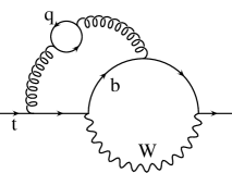
(a)	(b)

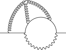
(c)

Figure 1: Examples of diagrams whose cuts contribute to the $\mathcal{O}(\alpha_{s}^{2})$ decay rate for $t\rightarrow bW$: (a) light or heavy quarks; (b) abelian; (c) non-abelian.

This difficult task can be organized in the following way. First, we perform a reduction of the original integrals to a set of simpler master integrals. In this phase we use the so-called integration-by-parts identitiesFyodor which lead to a system of recurrence relations between various loop integrals. The solution of such a system provides reduction formulas which allow us to express the original loop integrals in terms of master integrals.

There are two main paradigms for solving the system of recurrence relations. In the traditional method, one inspects the structure of the identities and rearranges them manually for an efficient iterative solution of the system. This “by inspection” method has proven to be very successful in numerous applications (see, e.g., vanRittbergen1 – Broadhurst ) but requires much human effort to implement. A newer method is based on the Gaussian elimination of a large system of identities with a given ordering function which measures the “difficulty” of each integral Laporta . This approach is fully automated and process-independent, but requires significant computing power. Thanks to an effective implementation and the growing performance of hardware, this method has become feasible at NNLO quite recently. In the present project we used both methods in parallel. We obtained identical results which serve as a crosscheck for the calculation. It also allows us to compare the two approaches and point out strengths and weaknesses of both.

The final step is the evaluation of the master integrals arising in the problem. For $t\rightarrow bW$ at $\mathcal{O}(\alpha_{s}^{2})$ there are $23$ master integrals which have been computed analytically.

III Results

Taking advantage of the tools discussed in the previous section, we can obtain the decay rate in the form of an expansion around the limit $m_{W}=m_{b}=0$ in the parameter $\omega=(m_{W}/m_{t})^{2}$ (see toppaper ). The decay width can be written in the following form:

$$\Gamma(t\rightarrow bW)=\Gamma_{0}\left[X_{0}+\frac{\alpha_{s}}{\pi}X_{1}+\left(\frac{\alpha_{s}}{\pi}\right)^{2}X_{2}\right],$$ (1)

where

$$\Gamma_{0}\equiv\frac{G_{F}m_{t}^{3}\left|V_{tb}\right|^{2}}{8\sqrt{2}\pi},$$ (2)

$X_{0}$ corresponds to the Born decay rate and $X_{1}$ is the already known NLO correction. Our goal in the present calculation is the coefficient $X_{2}$, which can be subdivided into four gauge-invariant color pieces:

$$X_{2}=C_{F}\left(T_{R}N_{L}X_{L}+T_{R}N_{H}X_{H}+C_{F}X_{A}+C_{A}X_{NA}\right),$$ (3)

where $C_{F}=4/3$, $C_{A}=3$, and $T_{R}=1/2$ are the usual SU(3) color factors and $N_{L}$ and $N_{H}$ denote the number of light $(m_{q}=0)$ and heavy $(m_{q}=m_{t})$ quark flavors.

We obtained series coefficients to $\omega^{5}$ analytically. In terms of numerical values our expansion reads:

$$X_{2}=-12.579+3.743\,\omega+6.054\,\omega^{2}+5.619\,\omega^{2}\log\omega+\mathcal{O}(\omega^{3}).$$ (4)

It is a straightforward task to improve the accuracy of an expansion by computing more terms in $\omega$. Moreover, the present expansion can be smoothly matched with the one in the zero recoil kinematics studied previously Czarnecki in the context of semileptonic b quark decays. The result of such a matching procedure is depicted in Fig. 2.

Figure 2: Matching of expansions around $\omega=0$ (thick line) and $\omega=1$ (thin line). The solid line denotes the resulting decay width valid in the full range of $\omega$.

For the measured ratio of the $W$ and top masses pdg , $\omega\simeq 0.213$, our expansion gives $X_{2}=-15.5(1)$, where the uncertainty is almost entirely due to the experimental error in the determination of $m_{t}$. The theoretical error, which originates from taking a finite number of terms in our expansion, is $20$ times smaller and can be reduced further if needed. Using $\alpha_{s}(m_{t})=0.11$, we find that the two-loop correction decreases the tree level decay rate by about $2\%$, in agreement with earlier expectations.

IV Conclusions

We have presented a new analytic $\mathcal{O}(\alpha_{s}^{2})$ result for the decay $t\rightarrow bW$ in terms of a parameter $\omega=(m_{W}/m_{t})^{2}$ and in the limit of $m_{b}=0$. This result has enabled us to confirm or modify slightly the corresponding results of previous numerical calculations. Our formulas are readily applicable to other physical processes such as muon decay and the semileptonic $b$ quark decay $b\rightarrow ul\nu$.

Our results depend on the imaginary parts of a novel class of three-loop integrals, which we have obtained using two independent paradigms for the solution of large systems of recurrence relations. To the best of our knowledge, this is the first time that both approaches have been used simultaneously to obtain a new result, and an objective analysis of the strengths and weaknesses of each approach will increase the efficiency of other large calculations in the future.

Acknowledgements: I am grateful to F. Tkachov for fruitful collaboration in developing the dedicated computer algebra system used in this project as well as to I. Blokland and A. Czarnecki for reading the manuscript and helpful remarks. This research was supported by the Alberta Ingenuity and by the Natural Sciences and Engineering Research Council of Canada.

References

- (1) M. Jezabek and J. Kuhn, Nucl. Phys. B34, 1729 (1980).
- (2) A. Denner and T. Sack, Nucl. Phys. B358, 46 (1991). G. Eilam, R. Mendel, R. Migneron, and A. Soni, Phys. Rev. Lett. 66, 3105 (1991).
- (3) M. Jezabek and J. Kuhn, Phys. Rev. D48, 1910 (1993).
- (4) A. Czarnecki and K. Melnikov, Nucl. Phys. B544, 520 (1999).
- (5) K. G. Chetyrkin, R. Harlander, T. Seidensticker, and M. Steinhauser, Phys. Rev. D60, 114015 (1999).
- (6) F. V. Tkachov, Phys. Lett. B100, 65 (1981).
- (7) T. van Ritbergen and R. G. Stuart, Phys. Rev. Lett. 82, 488 (1999).
- (8) T. van Ritbergen, Phys. Lett. B454, 353 (1999).
- (9) A. Czarnecki and K. Melnikov, Phys. Rev. Lett. 88, 131801 (2002).
- (10) D. J. Broadhurst, Z. Phys. C54, 599 (1992).
- (11) S. Laporta, Int. J. Mod. Phys. A15, 5087 (2000).
- (12) I. Blokland, A. Czarnecki, M. Slusarczyk, and F. Tkachov, hep-ph/0403221.
- (13) K. Hagiwara et al., Phys. Rev., D66, 010001 (2002).