BRANECODE
A Program for Simulations of
Braneworld Dynamics

Abstract

We describe an algorithm and a C++ implementation that we have written and made available for calculating the fully nonlinear evolution of $5$D braneworld models with scalar fields. Bulk fields allow for the stabilization of the extra dimension. However, they complicate the dynamics of the system, so that analytic calculations (performed within an effective $4$D theory) are usually only reliable for static bulk configurations or when the evolution of the extra dimension is negligible. In the general case, the nonlinear $5$D dynamics can be studied numerically, and the algorithm and code we describe are the first ones of that type designed for this task. The program and its full documentation are available on the Web at http://www.cita.utoronto.ca/~jmartin/BRANECODE/ . In this paper we provide a brief overview of what the program does and how to use it.

I Introduction

Many extensions of the Standard Model have in common the presence of extra dimensions. This has to be contrasted with the fact that our world looks four dimensional, so one has to explain why the presence of the extra space has not yet been detected. The traditional answer has been that the extra space is compact and very small, so that the fields associated with its excitations are too heavy to be observable in accelerators or cosmology. More recently, it has been realized that ordinary matter and gauge interactions may be confined on lower dimensional submanifolds, known as branes. In this case, they could be four dimensional objects, even if the geometry of the theory is higher dimensional. The situation is different for gravity, which propagates in the whole bulk space. Several questions naturally arise, such as why a compact space would remain small while the three non-compact dimensions are undergoing cosmological expansion, or why the expansion of the universe we see is described by $3+1$ dimensional general relativity so well. The presence of extra dimensions may cause deviations from the standard FRW cosmology that is supported by observations.

In most cases, these two questions turn out to be intimately related. Only if the extra space is static can the evolution of the non-compact coordinates behave as in the standard four dimensional case. Hence, the dynamics of the hidden dimensions becomes a crucial ingredient in understanding the evolution of the ones we observe. In some particular cases, static bulk configurations can be achieved under the combined action of the bulk/brane gravity. In most realistic examples that could account for our observed four dimensional cosmology the stability is due to the presence of additional fields that acquire nontrivial configurations in the bulk. While the stabilization has to be effective at relatively “late” times, the first stages of our universe (before primordial nucleosynthesis, for instance) are much less constrained. The evolution of the bulk may have been significant at this phase, and this offers many new possibilities for phenomenology. This is particularly true with the addition of the fields responsible for the “late” time stabilization, since they constitute new dynamical degrees of freedom for the system.

While the above considerations are valid for all models with extra dimensions, significant computations have been performed in the framework of brane models. These models can be thought of as simplified, phenomenological (bottom-up) versions of branes in string theory. The string dynamics is ignored and the primary focus is on the classical dynamics from the point of view of General Relativity. Branes act as a source for the Einstein equations of the system, with their tension and possibly with the energy density of fields confined on them. Additional sources are a bulk cosmological constant, or the energy density of possible bulk fields. This set-up is sufficiently rich to describe very interesting situations. For example, inflation in braneworlds can acquire a nice geometrical interpretation, with the inflaton associated with the distance between different branes, the Hubble parameter scale associated with the induced curvature on the branes, and with reheating through radion oscillations.

Despite this great simplification, the whole dynamics is still very complicated, in particular when a bulk scalar field is present. In this case, analytical computations are typically performed within an effective $4$ dimensional theory, obtained after the extra dimension is integrated out, or perturbatively, using linearized analysis around simple backgrounds. While these studies are very useful when the extra space is static or quasi-static, they are not sufficient to describe the system when the evolution of the bulk is important. For example, systems that are stable at low energy (low curvature of the branes) can become unstable when the energy/curvature is increased. The stability/instability can be studied analytically. However, one cannot determine analytically where the system will evolve towards when the initial configuration turns out to be unstable.

For example, we numerically examined the dynamics of brane collisions and found that, as the branes approach each other, the spacetime of the bulk asymptotically approaches the Kasner-type solution.

Motivated by these limitations with the analytical treatment, we undertook a numerical study of these models. We developed a numerical algorithm, implemented in a C++ code, specifically designed for codimension one braneworlds, with a scalar field included in order to provide stabilization of the bulk at low energies. With the assumption of homogeneity and isotropy along the brane spatial coordinates ${\bf x}\,$ (corresponding to the standard assumption of homogeneity and isotropy of the non-compact coordinates), the problem is reduced to an effectively $2$ dimensional one. The independent variables are the bulk time $t$ and the bulk dimension $y$. The program integrates numerically the full set of Einstein equations in the bulk, together with the Israel junction conditions at two orbifold branes. We discretize the two dimensional spacetime (time and the bulk coordinate) and solve the bulk differential equations by finite-differencing them using the so-called leapfrog scheme. This algorithm is sufficient for our problem, and it provides a good compromise between accuracy and computational time (see Section II for more details). The two branes act as (one dimensional) boundaries of this space, and the junction conditions provide the boundary conditions for the system at each time-step. The solution of a boundary value problem is required to provide generic initial conditions that fulfill the constraint equations and the boundary conditions at the beginning of the evolution. In the static configurations we have mentioned above, this boundary value problem is significantly simpler than in the general case. The setup of initial conditions is explained in more detail in Section IV.

The first results obtained with the code have been presented in Martin:2003yh . We are now making the code public on the World Wide Web under the name BRANECODE. Its website is at http://www.cita.utoronto.ca/~kofman/BRANECODE/. The website for the program has documentation, including derivations of all the equations used in the program. Here we present a short summary of what the program does and what it can be used for. For more details see the website. Section II of this paper gives an overview of what the program is and how it works. Sections III and IV describe the evolution equations and the setting of initial conditions respectively. Section V describes some of the output generated by the program. The references section is limited to papers from our group related to the BRANECODE design and its first results Martin:2003yh ; Frolov:2003yi ; Kofman:2004tk ; Contaldi:2004hr ; Felder:2001da . See these papers for a more complete set of references.

II Overview and User Adjustable Files

In this Section we give an overview of the program and how to adjust it for a particular simulation. More details can be found in the documentation.

To work with the BRANECODE the user must specify a model, consisting of bulk and brane potentials for the scalar field, plus initial conditions for the field and the geometry. This information is encoded in a model file, which is a header file read in by the program. The file should be called model_numeric.h or model_analytic.h depending on whether the initial conditions are specified numerically or analytically. The model files contain the potentials and their first and second derivatives that are needed for the evolution of the bulk equations (III) and boundary conditions (5). For example, the BRANECODE distribution includes both a numeric and an analytic model file (with different initial conditions). The file model_analytic.h contains examples for branes in AdS and AdS-Schwarzschild geometries, whereas the file model_numeric.h we designed for the class of models with bulk scalar fields determined by the bulk and brane potentials

$$V(\phi) = \tfrac{1}{2}\,m^{2}\phi^{2}+\Lambda\,\,,$$

$${U}_{i}(\phi) = \tfrac{1}{2}M_{i}\left(\phi_{i}-\sigma_{i}\right)^{2}+\lambda_{i}\,\,.$$ (1)

A bulk cosmological constant and brane tensions is included as constant terms in these potentials. Most importantly, the program is designed to work for arbitrary potentials, different from (II). Other potentials $V(\phi)$, $U_{i}(\phi)$ can be implemented by modifying the corresponding lines in the model file. Aside from this file, the only other file that the user needs to modify is parameters.h, which contains all the parameters for a given run of the program. These include the number of grid points, the running time, and a number of other general variables specific to each run. There is also a parameter in this file that tells the program which type of model file to look for.

Given a specific model and set of parameters, the BRANECODE solves the system of equations of motions for the metric functions and the scalar field (III) along with the boundary conditions provided by the presence of the branes (5). The required functions are contained in the file equations.cpp.

The BRANECODE has built-in routines for outputting and plotting the metric fields, the scalar field, and derived quantities. These outputs are stored in ASCII files that can be read in and plotted by any standard plotting software. There are also options (set in parameters.h) to have the program call GNUPLOT to generate and display postscript plots of the data at runtime. (These options should only be chosen if the program is running on a computer with both GNUPLOT and GHOSTVIEW.) An example of this graphical output is shown in Fig. 1.

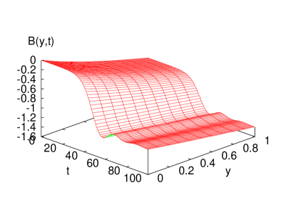
Figure 1: An example of the graphical output generated by the BRANECODE. The plot shows the evolution of a metric component $B$ (describing the interbrane separation) as a function of space and time. Physically, this evolution shows a transition from an unstable static warped geometry solution towards a stable static solution. During this non-linear reconfiguration the interbrane distance and the Hubble scale of the de Sitter geometry decreases.

Once all parameters have been set and you have modified or created a model file according to your wishes you simply compile and run the BRANECODE. The code is designed to be platform independent and should work with any C++ compiler. The makefile that comes with the distribution has entries and flags for the GNU gcc compiler and the INTEL icc compiler. You can select one of them or edit the makefile to invoke your favorite compiler.

III Algorithm

The evolution equations solved by the BRANECODE are the set of Einstein/scalar field equations on an effectively $2$ dimensional spacetime obtained after imposing homogeneity and isotropy on the non-compact spatial coordinates ${\bf x}\,$. In Martin:2003yh we showed that under these conditions it is always possible to choose coordinates that bring the metric to the form

$$ds^{2}={\rm e}^{2\,B\left(t,y\right)}\left(-dt^{2}+dy^{2}\right)+{\rm e}^{2\,A\left(t,y\right)}\,d{\bf x}^{2}\,\,,$$ (2)

with the two branes fixed at $y=0,\,1\,$, respectively. This choice is motivated by the fact that in this coordinate system the lattice size is time independent due to the fixed position of the branes and the equations simplify significantly. In this gauge, we have the following dynamical equations

$$\ddot{A\,\,}\!-A^{\prime\prime}+3\dot{A}^{2}-3A^{\prime 2} = \frac{2}{3}\,{\rm e}^{2B}V\,\,,$$

$$\ddot{B}-B^{\prime\prime}-3\dot{A}^{2}+3A^{\prime 2}+\frac{1}{2}\dot{\phi}^{2}-\frac{1}{2}{\phi^{\prime}}^{2} = -\frac{1}{3}{\rm e}^{2B}V\,\,,$$ (3)

$$\ddot{\phi}-\phi^{\prime\prime}+3\dot{A}\dot{\phi}-3A^{\prime}\phi^{\prime} = -{\rm e}^{2B}V_{,\phi}\,\,,$$

supplemented by the constraint equations

$$-A^{\prime}\dot{A}+B^{\prime}\dot{A}+A^{\prime}\dot{B}-\dot{A}^{\prime} = \frac{1}{3}\,\dot{\phi}\,\phi^{\prime}\,\,,$$ (4)

$$2A^{\prime 2}-A^{\prime}B^{\prime}+A^{\prime\prime}-\dot{A}^{2}-\dot{A}\dot{B} = -\frac{1}{6}{\dot{\phi}^{2}}-\frac{1}{6}{\phi^{\prime 2}}-\frac{1}{3}\,{\rm e}^{2B}V\,\,.$$

Dots and primes denote derivatives with respect to the time $t$ and the coordinate $y\,$ along the bulk, respectively. In addition, the program imposes the following junction (Israel) conditions at the positions of the branes

$$A^{\prime}=-\frac{1}{6}\,{U}\,{\rm e}^{B}\;,\;\;B^{\prime}=-\frac{1}{6}\,{U}\,{\rm e}^{B}\;,\;\;\phi^{\prime}=\frac{1}{2}{\rm e}^{B}\,U_{,\phi}\,\,.$$ (5)

These junction conditions are equivalent to extending the space beyond the two branes, and imposing ${\mathbb{Z}}_{2}$ symmetry across the branes.

In the coordinate system (2), the characteristic propagation speed of the dynamical equations is always $1$. This is advantageous from a numerical viewpoint as the size of the time step can be optimized uniformly by setting it equal to spatial grid separation. We describe below our implementation of the leapfrog discretization scheme, which is stable, second order accurate, and non-dissipative.

The program discretizes the $2$ dimensional $\left\{t,y\right\}$ space and computes the value of the three functions $B,\,A,\,\phi$ at each grid point. For any fixed time, the grid is made of $N+1$ points equally spaced along the bulk, with $0$ and $N$ corresponding to the locations of the two branes. The value of $N$ is set in parameters.h. The same grid spacing is taken in the $y$ and $t$ directions. The initial conditions are in the form $\left(A(y),B(y),\phi(y),\dot{A}(y),\dot{B}(y),\dot{\phi}(y)\right)\,$, and they can be chosen arbitrarily subject to the fact that they satisfy (4) and (5) at the initial time. Of particular interest are configurations with an initially static bulk, since the program can be used to verify their stability and to study the dynamics when they are unstable as described in section IV.

The discretized initial data $\left(\rule{0.0pt}{10.00002pt}A_{i}\right.$, $\dot{A}_{i}$, $B_{i}$, $\dot{B}_{i}$, $\phi_{i}$ , $\left.\dot{\phi}_{i}\rule{0.0pt}{10.00002pt}\right)\;,\;\;i=0,\dots,N$ has to be converted to a form suitable for the leapfrog algorithm. Instead of having the fields and their velocities at the time $t=t_{0}$, the algorithm needs the spatial profiles of the fields $(A_{i},B_{i},\phi_{i})$ at two subsequent moments in time $t=t_{0}$ and $t=t_{0}+\epsilon$. In some special cases the profiles at the two initial times can be calculated analytically, but in general the program takes a Runge-Kutta step using the initial derivatives to calculate the field values at $t_{0}+\epsilon$.

The field values at all subsequent time steps are calculated as follows. (Note that we will use $f$ here to denote a generic field, i.e. for equations that apply to all three fields $A$, $B$, and $\phi$.) In the gauge chosen, the bulk equations only contain derivatives in the form $\ddot{f}-f^{\prime\prime}\,$, and $\dot{f}\,\dot{g}-f^{\prime}\,g^{\prime}\,$. Recall that our grid spacing $\epsilon=1/N$ is equal to our time step. Thus, to second order accuracy, we can write the derivatives at a given point in spacetime in terms of the values of its neighbors as

$$\ddot{f}-f^{\prime\prime} = \frac{1}{\epsilon^{2}}\left(f_{\rm up}+f_{\rm dn}-f_{\rm lt}-f_{\rm rt}\right)+{\rm O}\left(\epsilon^{2}\right)\,\,,$$

$${\dot{f}}\,{\dot{g}}-{f^{\prime}}{g^{\prime}} = \frac{1}{4\,\epsilon^{2}}\left[\left(f_{\rm up}-f_{\rm dn}\right)\,\left(g_{\rm up}-g_{\rm dn}\right)+\right.$$ (6)

$$\left.-\left(f_{\rm rt}-f_{\rm lt}\right)\,\left(g_{\rm rt}-g_{\rm lt}\right)\right]+{\rm O}\left(\epsilon^{2}\right)\,\,,$$

where the indices label relative grid positions as defined in Fig. 2. In this way, the three differential equations (III) become three algebraic equations for the three unknown quantities $\left(B_{\rm up}\,,A_{\rm up}\,,\phi_{\rm up}\right)\,$. Notice that this can be done independently site by site in the bulk.

Once the bulk field values at the new time have been determined, we can apply the junction conditions (5) to advance the boundary field values. We discuss only the computation at the first brane ($i=0\,$). The treatment for the second brane is analogous. Only first derivatives in $y$ enter in (5). To preserve second order accuracy, we use an “asymmetric” discretization of the derivatives

$$f^{\prime}_{0} = \frac{1}{2\,\epsilon}\left(-\,3\,f_{0}+4f_{1}-f_{2}\right)+{\rm O}\left(\epsilon^{2}\right)\,\,,$$ (7)

where subscripts indicate the grid position of each field value (see Fig. 2). The junction conditions (5) thus become a set of three algebraic equations in terms of three unknowns. We can eliminate $A_{0}$ and $B_{0}$ in favor of $\phi_{0}\,$, and write an equation in terms of the only unknown quantity $\phi_{0}\,$,

$$4\,\phi_{1}-\phi_{2}-3\,\phi_{0}-\epsilon\,e^{B_{0}(\phi_{0})}\,{U}_{0}^{\prime}(\phi_{0})=0\,\,.$$ (8)

For specific brane potentials, these equations can be solved analytically. However, as the code is designed for arbitrary bulk/brane potentials, eq. (8) is solved numerically using the iterative Newton’s method. Once $\phi_{0}$ is determined, the remaining unknowns $B_{0}$ and $A_{0}$ are trivially computed through the remaining junction conditions.

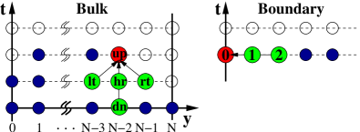
Figure 2: Numerical evolution scheme. See text for details.

IV Initial conditions

In general, the specification of initial conditions, i.e. the determination of the initial spatial profiles for the fields and their velocities $A(y)$, $B(y)$, $\phi(y)$, $\dot{A}(y)$, $\dot{B}(y)$, and $\dot{\phi}(y)$ is a non-trivial task. These function cannot be chosen independently, but rather are subject to the constraint equations (4) and boundary conditions (5). However, the physical instability of static de Sitter configurations Frolov:2003yi ; Martin:2003yh provides the possibility to generate interesting braneworld dynamics with static solutions as initial conditions that we can recommend. All the static solutions for a given model can be exhaustively classified by the phasespace analysis of the dynamics of the gravity/scalar system performed in Felder:2001da .

One simple way to generate static initial conditions is to consider a configuration of the form $B=B\left(y\right)\,,\;\phi=\phi\left(y\right)\,,\;A=B+H\,t\,$ (de Sitter branes in a static bulk). The first of the equations (4) is then trivially satisfied. For a sufficiently simple model, the remaining constraint equation can be solved analytically. Otherwise we provide a MATHEMATICA notebook and MAPLE worksheet to solve them numerically for a given bulk potential and generate appropriately formatted initial data. For simplicity, the code determines two of the three parameters of the brane potentials (II) in such a way that the boundary conditions (5) are fulfilled initially. The third parameter, either the tension on the brane $\lambda_{i}$ or the minimum of the brane potential $\sigma_{i}$, is set by the user in the file model_numeric.h. If the user instead wants to set up initial conditions for a given choice of brane potentials, he can make use of a shooting method operating in the phasespace of the static solutions. Namely, he can start with initial conditions chosen such that they fulfill the boundary conditions on one of the branes, compute the corresponding bulk configuration, and keep varying the initial conditions (e.g. with a numerical scan) until the solution also satisfies the junction conditions at the second boundary. For any given set of bulk and brane potentials, there can be none, one, or more than one solution to the boundary value problem. The latter case opens up the possibility for interesting dynamics of transitions as investigated in Martin:2003yh .

V Output

The main outputs of the program are the values of the three functions $B,\,A$, and $\phi$ at different bulk sites and time steps. Two parameters inside parameters.h control how many points (both in the $y$ and $t$ directions) are to be saved. From these quantities, one can construct some outputs of immediate physical relevance. One is the physical interbrane distance. The branes are at a fixed coordinate distance in our gauge and their physical separation is encoded in the metric coefficient $B\,$.

$$D\left(t\right)\equiv\int_{0}^{1}dy\,\sqrt{g_{55}}=\int_{0}^{1}dy\,{\rm e}^{B\left(t,\,y\right)}\ .$$ (9)

Another interesting quantity is the Hubble parameter as computed by observers on each of the two branes

$$H_{i}\equiv\frac{1}{a}\,\frac{d\,a}{d\,\tau}\Big{|}_{i}={\rm e}^{-B_{i}}\,\dot{A}_{i}\,\,,$$ (10)

where $\tau$ is the physical time measured by the observers, defined by $D\tau\equiv{\rm e}^{B}\,dt\,$. Quite interestingly, the gauge choice used in the algorithm (see the previous Section) does not exhaust the gauge freedom of the problem. Residual gauge transformations have been described in Martin:2003yh , and one can show that they do not change the values of $D$ and $H_{i}\,$, which therefore have physical meaning. Besides these physical quantities the BRANECODE also computes the Ricci scalar and the square of the Weyl tensor in the bulk. Other quantities of interest can easily be obtained from the “raw” values of $B,A,\phi$.

VI Conclusions

The main motivation for our work was to extend the knowledge of braneworld dynamics beyond the few situations where it was known analytically. Apart from these situations (characterized by a static or slowly evolving bulk), approximate methods based on effective $4$ dimensional computations are unreliable. In this short note we have presented an algorithm, together with its C++ implementation, designed for numerical computations in this framework. First results obtained from this code were presented in Martin:2003yh ; Kofman:2004tk . We could show that some bulk configurations which are stable at low energy (low value of the expansion rate $H$ of the two branes) become unstable as $H$ increases, in agreement with the analytical calculations of Frolov:2003yi . This can be interpreted as a part of a more general phenomenon of gravitational instability of compactification to four dimensional de Sitter geometry Contaldi:2004hr . The numerical integration allowed us to follow the evolution of the system starting from the unstable configuration. For certain bulk/brane potentials the system may evolve towards another static, but stable configuration, characterized by a lower value of $H$. The transition is typically a process of quick bulk reconfiguration. In many cases, however, the second configuration does not exist or cannot be reached. The two branes then either move apart to infinite distance, or they collide. Brane collisions is a very interesting subject by itself. The study of the numerical evolution led us to the conclusion that the asymptotic geometry is given by the universal Kasner-type that is typical of homogeneous but anisotropic strong gravity regimes. We did not investigated the case of branes departing from each other when one of them in general approaches a naked singularity in the bulk configuration. We also did not studied the possibility of the formation of an apparent horizon between the branes.

Our algorithm is focused on the simplest possible set-up which allows for brane stabilization based on a generalized Goldberger-Wise mechanism. Only one bulk scalar field has been considered, although with arbitrary potentials in the bulk and at the two branes. The inclusion of more scalar fields would be straightforward. In particular, one could consider other fields, which are confined to the branes, and which are coupled to the bulk fields e.g. through the brane potentials. (The interplay between bulk/brane fields may lead to novel interesting features not considered in Martin:2003yh ). Another easy generalization would be the inclusion of perfect fluids on the branes (for example, describing standard matter and radiation). Less trivial but more interesting extensions could be the inclusion of other types of fields (form fields in the bulk, for instance), or evolution with more dimensions included. For example, relaxing the hypothesis of homogeneity and isotropy along the ordinary dimensions would allow the study of inhomogeneous perturbations of the system.

References

- (1) J. Martin, G. N. Felder, A. V. Frolov, M. Peloso and L. Kofman, “Braneworld dynamics with the BraneCode,” Phys. Rev. D, to appear, [hep-th/0309001].
- (2) G. N. Felder, A. V. Frolov and L. Kofman, “Warped geometry of brane worlds,” Class. Quant. Grav. 19, 2983 (2002) [hep-th/0112165].
- (3) A. V. Frolov and L. Kofman, “Can inflating braneworlds be stabilized,” Phys. Rev. D 69, 044021 (2004) [hep-th/0309002].
- (4) L. Kofman, J. Martin and M. Peloso, “Exact identification of the radion and its coupling to the observable sector,” [hep-ph/0401189].
- (5) C. Contaldi, L. Kofman and M. Peloso, “Gravitational Instability of de Sitter Compactifications,” [hep-th/0403270].