A model for the spacetime evolution of heavy-ion collisions at RHIC

Abstract

We investigate the space-time evolution of ultrarelativistic Au-Au collisions at full RHIC energy using a schematic model of the expansion. Assuming a thermally equilibrated system, we can adjust the essential scale parameters of this model such that the measured transverse momentum spectra and Hanbury-Brown Twiss (HBT) correlation parameters are well described. We find that the experimental data strongly constrain the dynamics of the evolution of the emission source although hadronic observables for the most part reflect the final breakup of the system.

I Introduction

Numerical simulations of finite temperature Quantum Chromodynamics (QCD) on discrete space-time lattices suggest that the theory exhibits a transition to a new state of matter, the quark-gluon plasma (QGP), at temperatures of the order of 170 MeV Lattice . Experimentally, hadronic matter at this temperature can only be created for a short time in ultrarealtivistic heavy-ion collisions, and currently there are ongoing efforts from both experiment and theory to find conclusive evidence for the creation of the QGP and ultimately to study its properties. A wealth of data on hadronic single particle distributions and two particle correlations has been assembled so far.

In the interpretation of experimental data of ultrarelativistic heavy-ion collisions, however, one is often faced with the challenge to disentangle signals of new physics indicating the production of a QGP from known hadronic effects. This question can only be reliably addressed if the space-time evolution of the fireball created in the collision is sufficiently known. In this note, we present an attempt to determine the evolution of the bulk hadronic matter by fitting the essential scales of a schematic model for the fireball expansion dynamics to the measured hadronic data. The resulting scenario can then be used in the calculation of other observables (not used in the fit) which are sensitive to the bulk matter expansion, such as the emission of dileptons and photons or jet quenching, thus reducing or eliminating the inherent ambiguity in the interpretation mentioned above.

II The model

The main assumption for the model is that an equilibrated system is formed a short time $\tau_{0}$ after the onset of the collision. Furthermore, we assume that this thermal fireball subsequently expands isentropically until the mean free path of particles exceeds (at a timescale $\tau_{f}$) the dimensions of the system and particles move without significant interaction to the detector. In addition to this final breakup (freeze-out) of the fireball, particles are emitted throughout the expansion period whenever they cross the boundary of the thermalized fireball matter.

For simplicity we restrict the discussion to a system exhibiting radial symmetry around the beam (z)-axis corresponding to a central ($b=0$) collision. For the entropy density at a given proper time we make the ansatz

$$s(\tau,\eta_{s},r)=NR(r,\tau)\cdot H(\eta_{s},\tau)$$ (1)

with $\tau$ the proper time as measured in a frame co-moving with a given volume element and $\eta_{s}=\frac{1}{2}\ln(\frac{t+z}{t-z})$ the spacetime rapidity and $R(r,\tau),H(\eta_{s},\tau)$ two functions describing the shape of the distribution and $N$ a normalization factor. We use Woods-Saxon distributions

$$\begin{split}&R(r,\tau)=1/\left(1+\exp\left[\frac{r-R_{c}(\tau)}{d_{\text{ws}}}\right]\right)\\ &H(\eta_{s},\tau)=1/\left(1+\exp\left[\frac{\eta_{s}-H_{c}(\tau)}{\eta_{\text{ws}}}\right]\right).\end{split}$$ (2)

to describe the shapes for a given $\tau$. Thus, the ingredients of the model are the skin thickness parameters $d_{\text{ws}}$ and $\eta_{\text{ws}}$ and the parametrizations of the expansion of the spatial extensions $R_{c}(\tau),H_{c}(\tau)$ as a function of proper time. For simplicity, we assume for the moment a radially non-relativistic expansion and constant acceleration, therefore we find $R_{c}(\tau)=R_{0}+\frac{a_{\perp}}{2}\tau^{2}$. $H_{c}(\tau)$ is obtained by integrating forward in $\tau$ a trajectory originating from the collision center which is characterized by a rapidity $\eta_{c}(\tau)=\eta_{0}+a_{\eta}\tau$ with $\eta_{c}=\text{atanh }v_{z}^{c}$ the longitudinal expansion velocity for that trajectory. Since the relation between proper time as measured in the co-moving frame and lab time is determined by the rapidity at a given time, the resulting integral is in general non-trivial and solved numerically (see Synopsis for details). $R_{0}$ is determined in overlap calculations using Glauber theory, the initial size of the rapidity interval occupied by the fireball matter. $\eta_{0}$ is a free parameter and we choose to use the transverse velocity $v_{\perp}^{f}=a_{\perp}\tau_{f}$ and rapidity at decoupling proper time $\eta^{f}=\eta_{0}+a_{\eta}\tau_{f}$ as parameters. Thus, specifying $\eta_{0},\eta_{f},v_{\perp}^{f}$ and $\tau_{f}$ sets the essential scales of the spacetime evolution and $d_{\text{ws}}$ and $\eta_{\text{ws}}$ specify the detailed distribution of entropy density. For simplicity, we do not discuss a (possible) time dependence of the shapes (e.g. parametrized by $d_{\text{ws}}(\tau)$ and $\eta_{\text{ws}}(\tau)$) at this point.

We require that the parameter set $(\eta_{f},\eta_{\text{ws}})$ reproduces the experimentally observed rapidity distribution of particles Brahms-dN-deta but we do not make any assumptions about the initial rapidity interval characterized by $\eta_{0}$. This allows for the possibility of accelerated longitudinal expansion and implies in general $\eta\neq\eta_{s}$. Here, $\eta=\frac{1}{2}\ln\frac{p_{0}+p_{z}}{p_{0}-p_{z}}$ denotes the longitudinal rapidity of a volume element moving with momentum $p^{\mu}$. We require that the longitudinal flow profile is such that an initially homogeneous distribution remains homogeneous. For a general accelerated motion, there is no simple analytical expression for the spacetime position of sheets of given $\tau$ or the flow profile corresponding to $\tau=\sqrt{t^{2}-z^{2}}$ and $\eta=\eta_{s}$ valid for the non-accelerated case. In Synopsis however, we have investigated such an expansion pattern with a constant acceleration and argued that for rapidities $<4$ the acceleration leads to an approximately linear relation $\eta\approx\zeta\eta_{s}$ at given $\tau$ and that sheets of constant proper time are approximately hyperbolae as in the non-accelerated case. This mismatch between $\eta$ and $\eta_{s}$ leads to additional Lorentz contraction factors in volume integrals at given $\tau$, hence the longitudinal extension of matter on a sheet of given $\tau$ in the interval $-\eta_{s}^{\text{front}}<\eta_{s}<\eta_{s}^{\text{front}}$ must then be calculated as

$$L(\tau)\approx 2\tau\frac{\text{sinh }(\zeta-1)\eta_{s}^{\text{front}}}{(\zeta-1)}.$$ (3)

In the following, we use these results in our computations whenever $\eta_{f}\neq\eta_{0}$. For $\eta_{f}=\eta_{0}$, the model reduces to the well-known expressions of the Bjorken expansion scenario, e.g. $L(\tau)=2\eta_{0}\tau$ with $\tau=\sqrt{t^{2}-z^{2}}$.

For transverse flow we assume a linear relation between radius $r$ and transverse rapidity $\rho=\text{atanh }v_{\perp}(\tau)=r/R_{c}(\tau)\cdot\rho_{c}(\tau)$ with $\rho_{c}(\tau)=\text{atanh }a_{\perp}\tau$. For the net baryon density inside the fireball matter we assume a transverse distribution (apart from a normalization factor) given by $R(r,\tau)$, but its longitudinal distribution we parametrize such as to describe the measured data Brahms .

We proceed by specifying the equation of state (EoS) of the thermalized matter. In the QGP phase, we use an equation of state based on a quasiparticle interpretation of lattice QCD data (see Quasiparticles ). In the hadronic phase, we adopt the picture of subsequent chemical freeze-out (at the transition temperature $T_{C}$) and thermal freeze-out (at breakup temperature $T_{F}$) and consequently use a resonance gas EoS which depends on the local net baryon density. The reason for this is that a finite baryochemical potential $\mu_{B}$ leads to an increased number of heavy resonances at the phase transition point, and decay pions from these resonance decays lead in turn to a finite pion chemical potential $\mu_{\pi}$ in the late evolution phases which implies an overpopulation of pion phase space and faster cooling as compared to a scenario in chemical equilibrium. We calculate the pion chemical potential as a function of the local baryon and entropy density using the statistical hadronization framework outlined in Hadrochemistry . We find $\mu_{\pi}$ to be small ($\mathcal{O}(30\text{ MeV})$) in the midrapidity region at RHIC, however the corrections to the chemically equilibrated case are important.

With the help of the EoS, we can find the local temperature $T(\eta_{s},r,\tau)$ of a volume element from its entropy density $s(\eta_{s},r,\tau)$ and net baryon density $\rho_{B}(\eta_{s},r,\tau)$. We calculate particle emission throughout the whole lifetime of the fireball by selecting a freeze-out temperature $T_{f}$, finding the hypersurface characterized by $T(\eta_{s},r,\tau)=T_{f}$ and evaluating the Cooper-Frye formula

$$E\frac{d^{3}N}{d^{3}p}=\frac{g}{(2\pi)^{3}}\int d\sigma_{\mu}p^{\mu}\exp\left[\frac{p^{\mu}u_{\mu}-\mu_{i}}{T_{f}}\right]=d^{4}xS(x,p)$$ (4)

with $p^{\mu}$ the momentum of the emitted particle and $g$ its degeneracy factor. Note that the factor $d\sigma_{\mu}p^{\mu}$ contains the spacetime rapidity $\eta_{s}$ and the factor $p^{\mu}u_{\mu}$ the rapidity $\eta$. Since these are in general not the same in our model, the analytic expressions valid for a boost-invariant scenario ThermalPhenomenology do not apply.

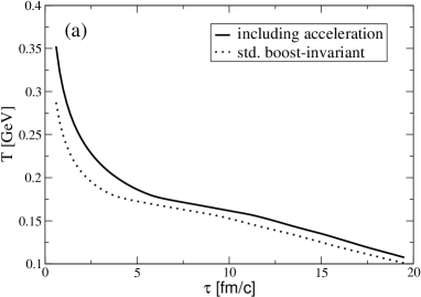
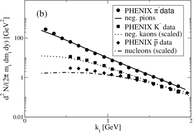
Figure 1: Left panel: Time evolution of the average fireball temperature for the fitted set of parameters (solid line) and a model assuming boost-invariant longitudinal expansion (dotted). Right panel: Measured transverse momentum spectra for $\pi^{-}$ (circles), $K^{-}$ (squares) and $\overline{p}$ (diamonds) as compared to the model results.

In our case, the parameter $\tau_{f}$ denotes the freeze-out time for the last volume element to reach the temperature $T_{f}$. Volume elements freeze out throughout the whole evolution time (and are boosted with a time- and position dependent flow velocity) whenever they cross the Cooper-Frye hypersurface. Therefore the transverse expansion parameter $v_{\perp}^{f}$ also does not necessarily reflect the typical transverse velocity of a volume element since freeze-out may occur earlier than $\tau_{f}$ and not at the radius $r=R(\tau)$.

Using this emission function, we calculate the HBT parameters as HBTReport ; HBTBoris

$$R_{\text{side}}^{2}=\langle\tilde{y}^{2}\rangle\quad R_{\text{out}}^{2}=\langle(\tilde{x}-\beta_{\perp}\tilde{t})^{2}\rangle\quad R_{\text{long}}=\langle\tilde{z}^{2}\rangle$$ (5)

with $\tilde{x}_{\mu}=x_{\mu}-\langle x_{\mu}\rangle$ and

$$\langle f(x)\rangle(K)=\frac{\int d^{4}xf(x)S(x,K)}{\int d^{4}xS(x,K)}$$ (6)

In order to parametrize the spacetime evolution of a central 200 AGeV Au-Au collision at RHIC we fit the remaining set of parameters $d_{\text{ws}},\eta_{0},T_{F}$ and $v_{\perp}^{f}$ to the experimentally obtained single particle transverse momentum spectra Phenix-HBT and HBT parameters Phenix-Spectra . For the description of the HBT correlation parameters which are measured for 30% central collisions, we scale down the entropy content and initial overlap radius guided by overlap calculations and neglect the angular asymmetry.

III Results and discussion

We find that the choice of parameters $T_{f}$ = 110 MeV, $d_{\text{ws}}<$ 1.0 fm, $\eta_{0}$ = 1.8 and $v_{\perp}^{f}=0.67$ is able to give a good description of the data. The resulting average cooling curve (computed by averaging the entropy density over the fireball volume at a given proper time and determining the corresponding temperature, where we define the fireball volume at given $\tau$ as the 3-volume bounded by the Cooper-Frye surface) and the transverse momentum spectra for $\pi^{-},K^{-}$ and nucleons are shown in Fig. 1, the HBT correlation parameters in Fig. 2.

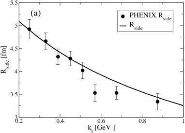
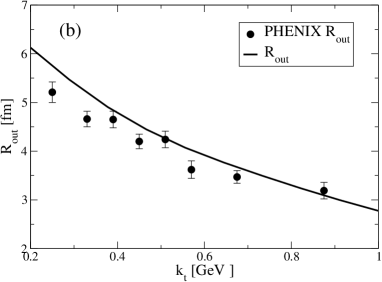
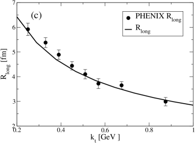
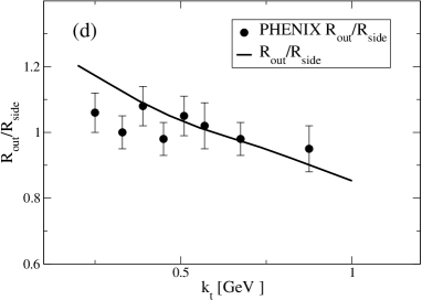
Figure 2: The HBT correlation parameters $R_{\text{side}},R_{\text{out}},R_{\text{long}}$ and the ratio $R_{\text{out}}/R_{\text{side}}$ in the model calculation as compared to PHENIX data Phenix-HBT .

The fit apparently misses the low $p_{t}$ part of the transverse momentum spectra for the heavier particles but describes the $\pi^{+}\pi^{+}$ correlation radii well, with the exception of the low $p_{t}$ part of $R_{\text{out}}$ where the calculation lies somewhat above the data.

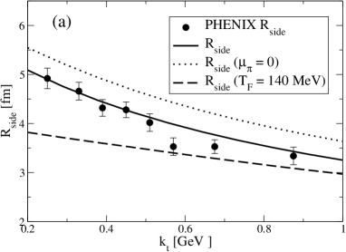
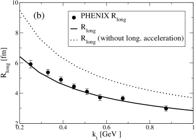
Figure 3: Left panel: $R_{\text{side}}$ in a scenario with vanishing pion chemical potential $\mu_{\pi}$ (dotted line) and a difference scenario assuming $T_{f}=140$ MeV (dashed line) as compared to the standard calculation (solid) Right panel: $R_{\text{long}}$ in a scenario with $T_{f}$ = 110 MeV but assuming no longitudinal acceleration (dotted) compared with the standard scenario (solid). Note that the transverse momentum spectra are well described by all of the scenarios shown in this figure.

The rather steep falloff of $R_{\text{side}}$, $R_{\text{out}}$ as a function of $k_{t}$ favours a large amount of flow. However, demanding simultaneous agreement with the slope of the momentum spectra implies that large transverse flow has to be accompanied by low freeze-out temperatures. Therefore, the volume at freeze-out has to be large in order to reach small entropy densities. The inclusion of a finite pion chemical potential (originating from resonance decays in chemical non-equilibrium) is crucial to reduce the volume corresponding to a given average temperature. Since the radial expansion is rather constrained by the normalization of the HBT parameters, a large volume implies sizeable longitudinal extension and hence a long-lived system. Such a long lifetime in combination with a standard boost-invariant longitudinal expansion leads to large values of $R_{\text{long}}$ which are clearly incompatible with the data. A sizeable longitudinal compression and re-expansion however leads to a reasonable description of $R_{\text{long}}$ as well.

It is not possible to identify a single feature of the model as being responsible for the good quality of the fit but one can illustrate certain trends. Neglecting the additional cooling caused by a finite value of $\mu_{\pi}$, it is still possible to describe the spectra and the slope of the HBT data well for a low freeze-out temperature, however a larger volume is needed to get to this temperature and therefore the normalization of the correlation radii is systematically above the data (see Fig. 3, left panel).

On the other hand, retaining the idea of a boost-invariant scenario without longitudinal acceleration implies a short lifetime of the system as apparent from the estimate $R_{\text{long}}=\tau_{f}(T_{f}/m_{t})^{1/2}$ based on such an expansion pattern. Such a short lifetime can be achieved by a large value of $T_{f}$. The transverse expansion velocity can then be adjusted to fit the $m_{t}$ spectra, but the resulting solution is characterized by small flow velocities which leave both normalization and falloff of $R_{\text{side}}$ in disagreement with the data (see Fig. 3, left panel). Retaining a low freeze-out temperature in a boost-invariant scenario allows to describe the transverse spectra and correlations well but significantly overpredicts $R_{\text{long}}$ (see Fig. 3, right panel).

Concluding, we find that the $m_{t}$ spectra and HBT parameters measured at RHIC can be simultaneously described assuming a scenario with small freeze-out temperature $T_{F}\approx 110$ MeV and a sizeable initial longitudinal compression and re-expansion. The data strongly constrain alternative scenarios. An upcoming publication will investigate the dependence of the results on the different model parameters in more detail. The calculation of further observables reflecting different properties of the fireball expansion such as the emission of electromagnetic probes or the suppression of high $p_{t}$ jets within the same framework will help to confirm or disprove the outlined scenario.

- (1) F. Karsch, E. Laermann and A. Peikert, Phys. Lett. B 478 (2000) 447.
- (2) T. Renk, hep-ph/0403239.
- (3) I. G. Bearden et al. [BRAHMS Collaboration], Phys. Rev. Lett. 88 (2002) 202301.
- (4) I. G. Bearden et al. [BRAHMS Collaboration], nucl-ex/0312023.
- (5) R. A. Schneider and W. Weise, Phys. Rev. C 64 (2001) 055201; M. A. Thaler, R. A. Schneider and W. Weise, hep-ph/0310251.
- (6) T. Renk, Phys. Rev. C 68 (2003) 064901.
- (7) E. Schnedermann, J. Sollfrank and U. W. Heinz, Phys. Rev. C 48 (1993) 2462.
- (8) U. A. Wiedemann and U. W. Heinz, Phys. Rept. 319 (1999) 145.
- (9) B. Tomasik and U. A. Wiedemann, hep-ph/0210250.
- (10) S. S. Adler et al. [PHENIX Collaboration], nucl-ex/0401003.
- (11) S. S. Adler et al. [PHENIX Collaboration], nucl-ex/0307022.