Electroweak-scale inflation, inflaton–Higgs mixing and the scalar spectral index

Abstract

We construct a phenomenological model of electroweak-scale inflation that is in accordance with recent cosmic microwave background observations by WMAP, while setting the stage for a zero-temperature electroweak transition as assumed in recent models of baryogenesis. We find that the scalar spectral index especially poses tight constraints for low-scale inflation models. The inflaton–Higgs coupling leads to substantial mixing of the scalar degrees of freedom. Two types of scalar particles emerge with decay widths similar to that of the Standard Model Higgs particle.

• Keywords: inflation, physics of the early universe, baryon asymmetry, CMBR theory.

1 Introduction

With the results from the WMAP mission [1, 2] it has become relevant to critically review models of inflation, especially with regard to the scalar spectral index. While clearly still susceptible to improvement, the cosmic microwave background (CMB) observations are accurate enough to rule out certain (classes of) models, see e.g. [3, 4, 5]. In this paper we consider electroweak-scale inflation, which turns out to be indeed tightly constrained by the spectral index.

The motivation for looking at electroweak-scale (i.e. of order 100 GeV) inflation is twofold. Firstly, it is interesting to see if one can construct a working model of inflation with just minimal extensions of the Standard Model (SM) of particle physics, and to derive what kind of additional constraints such a coupling to the SM puts on an inflation model. The second (main) motivation has to do with baryogenesis, the production of the observed baryon asymmetry in the universe. As reviewed in [6], all necessary ingredients for baryogenesis (baryon number violation, C and CP violation, and non-equilibrium) are present in the SM. This provides a strong motivation for trying to construct a working model of electroweak baryogenesis. However, the current lore is that in a standard finite-temperature electroweak transition both the CP-violating and the non-equilibrium effects are too small to be able to account for the observed baryon asymmetry. These problems may be resolved in the context of tachyonic preheating at the electroweak scale after low-scale inflation [7, 8, 9, 10, 11, 12]. A tachyonic electroweak transition is strongly out of equilibrium, and the fact that the process takes place at zero temperature at the end of inflation may maximize the effectiveness of CP violation [13]. In addition, the low reheating temperature prevents sphaleron wash-out of the baryon number produced [6].

In this context it becomes important to check that the models that combine low-scale inflation with tachyonic electroweak preheating satisfy all the new observational constraints from WMAP. Low-scale inflation has been considered in many papers (see for instance [14, 15, 10, 16, 17]). In this paper we build in particular on [10], which was also motivated by the problem of electroweak baryogenesis. The main idea is that we have a kind of hybrid inflation model [18, 19], in which inflation is driven by a nearly constant potential energy of order (100 GeV)⁴ [7, 8], while one field (the inflaton) slowly rolls down its potential and the other field (the Higgs) is in a local minimum at zero. Once the inflaton passes a critical value, the local minimum for the Higgs field develops into a local maximum and both fields roll down rapidly to the absolute minimum at a non-zero value of the Higgs field, thus breaking the electroweak symmetry. As was shown in [10], ordinary hybrid inflation models in which the inflaton rolls from large field values towards zero are not viable at low scales because of large quantum loop corrections. This problem can be avoided in inverted hybrid inflation models, in which the inflaton rolls away from zero and inflation takes place at very small field values. Note that unlike standard hybrid inflation, slow-roll inflation ends in this case before the critical value is reached, instead of the end being caused by the phase transition, so that the slow-roll inflation stage and the phase transition can be considered as two separate processes.

The paper [10] was written before WMAP, and the authors did not study the spectral index. As we will show in this paper, their model gives a spectral index that is too low according to WMAP. In [16] somewhat more general low-scale inflation models were considered, although not from the point of view of electroweak baryogenesis, but these models still appear to be incompatible with WMAP. We shall show that one can improve these models to obtain a spectral index that lies comfortably within the WMAP confidence levels.

At first sight it may seem that one can always fine-tune a model with sufficient parameters to satisfy the constraints, but this is not necessarily the case within a set of reasonable rules. To formulate these rules we start from the point of view that we are constructing a purely phenomenological model, a minimal extension of the SM that introduces only one extra inflaton field in order to describe the history of the universe during and after inflation. We stress that there is nothing wrong with fine-tuned parameters in a phenomenological model, as the phenomenologically very successful SM shows. In incorporating a slow-roll inflationary regime compatible with the CMB measurements, one is led to an inflaton potential with non-renormalizable couplings. To constrain this potential we assume a polynomial approximation, such that there is only a limited number of terms to be parametrized.

This leads to a tight fit when we also incorporate the scenario of tachyonic electroweak baryogenesis, which requires that the inflaton field ends up far from the slow-roll regime with a vacuum expectation value similar to that of the Higgs field. The inflaton is a gauge singlet and it couples only to the radial (gauge-invariant) mode of the Higgs field. This coupling should induce a sufficiently fast tachyonic electroweak transition to make baryogenesis possible, without being unrealistically large. It implies a considerable mixing between the inflaton and Higgs modes, and the model predicts the existence of (only) two scalar particle species with electroweak-scale masses. Up to mixing-angle factors, their decay widths are similar to that of a SM Higgs with the same mass. The model should therefore be falsifiable by accelerator experiments, in particular with the LHC.

An important issue with any slow-roll inflation model is the question whether the assumed flatness of the effective potential is consistent with basic properties of quantum fields, with ‘quantum corrections’. We investigate this by calculating one-loop corrections to the effective potential. This exercise also led us to a rough estimate of the scale at which the model may be expected to break down because of its non-renormalizable and strong couplings.

The outline of the paper is as follows. In section 2 we first address the number of e-folds of inflation between horizon crossing of a WMAP-observable scale and the end of inflation, which number is crucial for the computation of CMB observables. Contrary to the generic situation, there is little uncertainty here because the (p)reheating of the universe and the onset of the radiation-dominated era are reasonably well understood in this model. Next, in section 3, we review the model of [10] and show that its spectral index disagrees with WMAP. The implied inflaton–Higgs mixing is studied in section 4. We then show in the following section (plus appendix A) that, by adding two additional terms to the potential and tuning the coupling parameters to a certain extent, values for the scalar spectral index in agreement with WMAP can be obtained. In section 6 (plus appendix B) we calculate one-loop quantum corrections to the effective potential and study the implications. Finally, section 7 summarizes our conclusions.

2 Number of e-folds

One of the most important differences between low-scale inflation and ‘normal’ inflation taking place around the GUT scale is that the number of e-folds $N_{k}$ of inflation between horizon crossing of the observationally relevant modes $k$ and the end of inflation is much lower. An expression for $N_{k}$ is derived as follows [20] (see also the recent papers [21, 22]):

$$\frac{k}{a_{0}H_{0}}=\frac{a_{\mathrm{H}}H_{\mathrm{H}}}{a_{0}H_{0}}=\frac{a_{\mathrm{H}}}{a_{\mathrm{e}}}\frac{a_{\mathrm{e}}}{a_{\mathrm{reh}}}\frac{a_{\mathrm{reh}}}{a_{\mathrm{eq}}}\frac{a_{\mathrm{eq}}}{a_{0}}\frac{H_{\mathrm{H}}}{H_{0}}=e^{-N_{k}}\left(\frac{\rho_{\mathrm{eq}}}{\rho_{\mathrm{reh}}}\right)^{1/4}(1+z_{\mathrm{eq}})^{-1}\,\frac{\kappa\rho_{\mathrm{H}}^{1/2}}{\sqrt{3}H_{0}}.$$ (1)

Here $a$ is the scale factor, $H\equiv\dot{a}/a$ the Hubble rate, $z$ is the redshift, the subscripts $0$, H, e, reh and eq denote evaluation now, at horizon crossing ($k=aH$), at the end of inflation, at the end of reheating and at radiation–matter equality, respectively, and $\kappa$ is the inverse reduced Planck mass, $\kappa^{2}\equiv 8\pi G$ ($\kappa^{-1}=2.436\times 10^{18}$ GeV). Here we used the fact that $\rho\propto a^{-4}$ during radiation domination and the Friedmann equation to rewrite $H_{\mathrm{H}}$. Furthermore we made use of the fact that electroweak (p)reheating is nearly instantaneous on the Hubble time scale at the end of inflation, $a_{\mathrm{e}}/a_{\mathrm{reh}}=1$, since its time scale is of order of 1 GeV^-1 for the SM degrees of freedom [23], whereas the Hubble time $H^{-1}$ at the end of electroweak-scale inflation is of order $10^{14}$ GeV^-1. At radiation–matter equality the energy density $\rho_{\mathrm{eq}}$ is twice that in non-relativistic matter, $\rho_{\mathrm{eq}}=2\Omega_{\mathrm{m}}(1+z_{\mathrm{eq}})^{3}\rho_{\mathrm{c}0}$, with $\rho_{\mathrm{c}0}$ the critical density at present, $\rho_{\mathrm{c}0}=3\kappa^{-2}H_{0}^{2}$. Moreover, in our model $\rho_{\mathrm{reh}}$, $\rho_{\mathrm{e}}$ and $\rho_{\mathrm{H}}$ are all practically equal, and so we find

$$N_{k}=-\ln\left(\frac{k}{a_{0}H_{0}}\right)+\frac{1}{4}\ln\left(\frac{2\Omega_{\mathrm{m}}}{3(1+z_{\mathrm{eq}})}\right)+\frac{1}{4}\ln\left(\frac{\kappa^{2}\rho_{\mathrm{H}}}{H_{0}^{2}}\right)=23.8,$$ (2)

where we used [1] $\Omega_{\mathrm{m}}=0.29$, $1+z_{\mathrm{eq}}=3455$, $H_{0}=73$ km/s Mpc^-1, the WMAP pivot scale of $k/a_{0}=0.05$ Mpc^-1 and an inflationary energy scale of $\rho_{\mathrm{H}}^{1/4}=100$ GeV. Hence, this number of e-folds $N_{k}$ is much smaller than the 50–60 one gets in the customary models where inflation takes place at much higher energy scales.

As we will show below, the scalar spectral index ${\tilde{n}}\equiv n-1$ is approximately inversely proportional to $N_{k}$. This means that the smaller $N_{k}$ of low-scale inflation makes it more difficult to satisfy the WMAP constraint that ${\tilde{n}}$ should be close to zero. More precisely the constraints from WMAP (including CBI and ACBAR, but no other experiments) for the amplitude $|\delta_{\mathbf{k}}|^{2}$ and spectral index ${\tilde{n}}$ of the CMB power spectrum are given by [1] (converted to our normalization, see the definitions in (6)):

$$|\delta_{\mathbf{k}}|^{2}=(3.8\pm 0.5)\times 10^{-10},\qquad\qquad{\tilde{n}}=-0.03\pm 0.03.$$ (3)

3 Core model

3.1 Model and WMAP constraints

The model proposed in [10] contains a scalar field $\sigma$ (the inflaton) in addition to the SM Higgs field $\phi$. The effective potential of the scalar fields has the form

$$V(\sigma,\phi)=V_{0}-\frac{1}{p}\alpha_{p}\sigma^{p}+\frac{1}{q}\alpha_{q}\sigma^{q}-\frac{1}{2}\lambda_{\sigma\phi}\sigma^{2}\phi^{2}+\frac{1}{2}\mu^{2}\phi^{2}+\frac{1}{4}\lambda_{\phi}(\phi^{2})^{2},$$ (4)

with integer $q>p>2$. The authors of [10] arrived at the values $p=5$, $q=6$. As we shall explain below, the value of $p$ is fixed by matching the inflationary (small $\sigma$) part of the potential to the SM physics part where $\sigma$ and $\phi$ are near their vacuum expectation values. First we need to establish the connection with the CMB data (3).

We choose the inflationary energy scale $V_{0}^{1/4}=100$ GeV. This choice guarantees that after preheating and thermalization, the temperature $T_{\mathrm{reh}}$ is substantially below the electroweak crossover temperature $T_{\mathrm{c}}\simeq 70$ GeV [24], thereby avoiding sphaleron washout of the generated baryon asymmetry. The reheating temperature can be estimated as $T_{\mathrm{reh}}=[30V_{0}/(\pi^{2}g_{*})]^{1/4}\simeq 0.43\,V_{0}^{1/4}$, with $g_{*}=86.25$ the effective number of SM degrees of freedom below the W mass.

Initial conditions are assumed such that the inflaton has a tiny but non-zero value $\sigma_{0}\raisebox{-0.43057pt}{ $\begin{array}[]{@{}c}\scriptstyle<\\ \scriptstyle\sim\end{array}$}10^{-10}$ GeV. The Higgs field is assumed to be in the ground state corresponding to this value of $\sigma$, i.e. $\phi=0$. Only when $\sigma$ reaches the critical value $\sigma_{\mathrm{c}}=\mu/\sqrt{\lambda_{\sigma\phi}}$, which happens long after inflation has ended in this model, will $\phi$ roll away from zero and break the electroweak symmetry. This means that we can consider the single-field slow-roll inflation stage and the phase transition as two separate processes.

At the tiny values of $\sigma$ relevant for inflation the $\sigma^{q}$ term in the potential is irrelevant. Taking only the first two terms into account, the model can be solved analytically in the slow-roll approximation in terms of the number of e-folds $N$ since the beginning of inflation:

$$\sigma_{,N}=-\frac{V_{,\sigma}}{3H^{2}}=\frac{\alpha_{p}\sigma^{p-1}}{\kappa^{2}V_{0}}\qquad\Rightarrow\qquad\sigma(N)=\left(\sigma_{0}^{2-p}+(2-p)\frac{\alpha_{p}}{\kappa^{2}V_{0}}\,N\right)^{\frac{1}{2-p}},$$

$${\tilde{\epsilon}}=\frac{1}{2}\kappa^{2}\left(\sigma_{,N}\right)^{2}=\frac{\alpha_{p}^{2}}{2\kappa^{2}V_{0}^{2}}\,\sigma^{2p-2},\qquad\qquad{\tilde{\eta}}=\frac{\sigma_{,NN}}{\sigma_{,N}}-{\tilde{\epsilon}}=(p-1)\frac{\alpha_{p}}{\kappa^{2}V_{0}}\,\sigma^{p-2},$$ (5)

where ${\tilde{\epsilon}}\equiv-\dot{H}/H^{2}$ and ${\tilde{\eta}}\equiv\ddot{\sigma}/(H\dot{\sigma})$ are the slow-roll functions, and we have used the fact that ${\tilde{\epsilon}}\ll{\tilde{\eta}}$, because $\alpha_{p}\sigma^{p}\ll V_{0}$ during inflation, to neglect the ${\tilde{\epsilon}}$ term in the expression for ${\tilde{\eta}}$, as well as to set $H^{2}=(\kappa^{2}/3)V_{0}$. Defining ${\tilde{\eta}}=1$ as the end of inflation, we can now compute the scalar amplitude and spectral index to leading order in slow roll (see e.g. [20, 25]):

$$|\delta_{\mathbf{k}}|^{2}=\frac{\kappa^{2}}{50\pi^{2}}\frac{H_{\mathrm{H}}^{2}}{{\tilde{\epsilon}}_{\mathrm{H}}}=\frac{1}{75\pi^{2}}\,\alpha_{p}^{\frac{2}{p-2}}\left(\kappa^{2}V_{0}\right)^{\frac{p-4}{p-2}}\left((p-1)+(p-2)N_{k}\right)^{\frac{2p-2}{p-2}},$$

$${\tilde{n}}=-2{\tilde{\eta}}_{\mathrm{H}}-4{\tilde{\epsilon}}_{\mathrm{H}}=-2\,\frac{(p-1)}{(p-1)+(p-2)N_{k}}\approx-\frac{2}{N_{k}}\frac{p-1}{p-2},$$ (6)

using again that ${\tilde{\epsilon}}_{\mathrm{H}}\ll{\tilde{\eta}}_{\mathrm{H}}$. Hence we see that ${\tilde{n}}$ is indeed approximately inversely proportional to $N_{k}$.

From (6) we see that the best (least negative) value one can get is ${\tilde{n}}=-0.084$ (in the limit of large $p$). Actually the situation is even worse than this, for two reasons. In the first place we find in numerical studies that generically there are about 2 more e-folds of inflation after ${\tilde{\eta}}=1$ has been reached, which means that one should use $N_{k}\simeq 22$ instead of $23.8$. Secondly, one cannot take an arbitrarily large $p$, because, as we will show below, $p>5$ is not compatible with the constraints from the Higgs sector. This means that the upper limit is actually ${\tilde{n}}=-0.114$ in this model, which is $3\sigma$ away from the WMAP result (3).

	$\alpha_{p}$	$\sigma_{\mathrm{e}}$ (GeV)	$\sigma_{\mathrm{H}}$ (GeV)	${\tilde{\epsilon}}_{\mathrm{e}}$
$p=4$	$2.71\times 10^{-12}$	$1.4\times 10^{-9}$	$3.6\times 10^{-10}$	$1.9\times 10^{-56}$
$p=5$	$1.51\times 10^{-3}$ GeV-1	$1.4\times 10^{-9}$	$5.4\times 10^{-10}$	$1.0\times 10^{-56}$
$p=6$	$6.75\times 10^{+5}$ GeV-2	$1.5\times 10^{-9}$	$7.2\times 10^{-10}$	$7.5\times 10^{-57}$

Table 1: Some quantities in the inflation model with potential $V=V_{0}-\frac{1}{p}\alpha_{p}\sigma^{p}$ with $V_{0}=(100$ GeV$)^{4}$ for $p=4,5,6$, as follow from applying the WMAP amplitude constraint for the mode that crossed the horizon at $N_{\mathrm{H}}$, defined as $N_{k}=22$ e-folds before the end of inflation $N_{\mathrm{e}}$.

The coefficient $\alpha_{p}$ is determined by fitting the amplitude (6) to the WMAP value (3). Results are given in table 1 for the cases of $p=4,5,6$. From this we can derive at which value $\sigma_{\mathrm{e}}$ of the inflaton slow-roll inflation ends (${\tilde{\eta}}=1$), and at which value $\sigma_{\mathrm{H}}$ horizon crossing of the scale under consideration occurs, see the table. Note that ${\tilde{\epsilon}}$ at the end of inflation, also given in the table, is still tiny.

3.2 Higgs sector

Next we look at the matching to the Higgs sector, i.e. we consider the stage after inflation when $\sigma$ has grown larger than $\sigma_{\mathrm{c}}$ and $\phi$ is no longer zero. Here we have the following constraints. Denoting the value of the fields in the absolute minimum by $v_{\sigma}$ and $v_{\phi}$, respectively, we have firstly the two conditions that the first derivatives of the potential with respect to $\sigma$ and $\phi$ in the point $(v_{\sigma},v_{\phi})$ vanish. Secondly, we demand that the second derivative with respect to $\phi$ in this point is equal to the the diagonal Higgs mass squared, $m_{\phi}^{2}$. The actual particle masses are to be obtained from a diagonalization of the $\sigma$–$\phi$ mass matrix, which we will discuss in section 4. Thirdly, there is the condition that $V(v_{\sigma},v_{\phi})=0$, so there is no residual vacuum energy (or it is at least negligible compared to the electroweak scale).

Taking $v_{\phi}$, $m_{\phi}$ and $\mu$ as additional input parameters, these four constraints lead to expressions for $\lambda_{\sigma\phi}$, $\lambda_{\phi}$, $\alpha_{q}$ and $v_{\sigma}$:

$$\lambda_{\sigma\phi}=\left(\mu^{2}+\frac{1}{2}m_{\phi}^{2}\right)v_{\sigma}^{-2},\qquad\lambda_{\phi}=\frac{m_{\phi}^{2}}{2v_{\phi}^{2}},\qquad\alpha_{q}=\left(\mu^{2}+\frac{1}{2}m_{\phi}^{2}\right)v_{\phi}^{2}v_{\sigma}^{-q}+\alpha_{p}v_{\sigma}^{p-q}.$$ (7)

The vacuum expectation value of the inflaton, $v_{\sigma}$, cannot be given analytically, but can easily be computed numerically from the condition that $V(v_{\sigma},v_{\phi})=0$, given the above relations. We take

$$v_{\phi}=246\;\mbox{GeV},\qquad\qquad m_{\phi}=200\;\mbox{GeV},\qquad\qquad\mu=100\;\mbox{GeV},$$ (8)

where $v_{\phi}$ is the usual SM value. The value for the Higgs mass is of course not known yet, but we require that the eigenvalues of the $\sigma$–$\phi$ mass matrix are above the current lower bound on the Higgs particle mass of 114 GeV [26]. It turns out that to satisfy this lower bound we need to choose a much larger value for the diagonal Higgs mass; 200 GeV will be sufficient.

A further condition comes from baryogenesis: the inflaton–Higgs coupling should be large enough that the tachyonic transition is sufficiently out of equilibrium. The rate of change of the effective Higgs mass squared when $\sigma$ crosses $\sigma_{\mathrm{c}}=\mu/\sqrt{\lambda_{\sigma\phi}}$ is determined by a dimensionless velocity parameter $u$:

$$u\equiv\frac{1}{2\mu^{3}}\,\frac{\partial(\mu^{2}-\lambda_{\sigma\phi}\sigma^{2})}{\partial t}=-\frac{\sqrt{\lambda_{\sigma\phi}}}{\mu^{2}}\,\frac{\partial\sigma}{\partial t},\qquad t=t_{\mathrm{c}},$$ (9)

where $t_{\mathrm{c}}$ is the time when $\sigma=\sigma_{\mathrm{c}}$. We have used $\mu$ to set the scale. The value of this mass is not critical here (although it may influence the precise value of the baryon asymmetry generated) and we have chosen $\mu=100$ GeV. We shall assume that $u\raisebox{-0.43057pt}{ $\begin{array}[]{@{}c}\scriptstyle>\\ \scriptstyle\sim\end{array}$}0.15$ for sufficient baryogenesis. The value of $u$ can be estimated from energy conservation [10]:

$$\frac{1}{2}\left(\frac{\partial\sigma}{\partial t}\right)^{2}=V_{0}-V(\sigma_{\mathrm{c}},0)\equiv cV_{0},\qquad 0<c<1\qquad\Rightarrow\qquad\lambda_{\sigma\phi}=\frac{\mu^{4}}{2cV_{0}}\,u^{2}.$$ (10)

Requiring $u\raisebox{-0.43057pt}{ $\begin{array}[]{@{}c}\scriptstyle>\\ \scriptstyle\sim\end{array}$}0.15$ means that $\lambda_{\sigma\phi}\raisebox{-0.43057pt}{ $\begin{array}[]{@{}c}\scriptstyle>\\ \scriptstyle\sim\end{array}$}0.01/c>0.01$ (for our choices $\mu=100$ GeV and $V_{0}^{1/4}=100$ GeV). On the other hand, $\lambda_{\sigma\phi}$ should not be too large in order to have radiative corrections under control, say $\lambda_{\sigma\phi}<1$.

From the expressions given in (7) and (8) we find the results given in table 2. Now we can draw the conclusion alluded to before: $p=5$ is the only value that satisfies all constraints. For $p\leq 4$ the coupling $\lambda_{\sigma\phi}$ between the inflaton and the Higgs is too small for baryogenesis, while this case is also worse for the scalar spectral index ${\tilde{n}}$. For $p\geq 6$, $\lambda_{\sigma\phi}$ is much too large, making quantum corrections uncontrollable. Note that even the extreme $p=6$ case with $q=7$, $\mu=1$ GeV and $m_{\phi}=132$ GeV (which means that the smallest eigenvalue of the $\sigma$–$\phi$ mass matrix is 115 GeV) gives a $\lambda_{\sigma\phi}$ that is still much too large ($\lambda_{\sigma\phi}=625$), so that this conclusion does not depend on our parameter choices. Hence, we really cannot go beyond $p=5$ when we try to maximize the spectral index.

	$\lambda_{\sigma\phi}$	$\lambda_{\phi}$	$\alpha_{q}$	$v_{\sigma}$ (GeV)
$p=4$, $q=6$	$1.4\times 10^{-6}$	0.33	$3.2\times 10^{-22}$ GeV-2	$1.45\times 10^{5}$
$p=5$, $q=6$	0.36	0.33	$8.4\times 10^{-6}$ GeV-2	288
$p=6$, $q=7$	$2.0\times 10^{3}$	0.33	$3.0\times 10^{+5}$ GeV-3	3.90
$p=6$, $q=8$	$3.1\times 10^{3}$	0.33	$2.9\times 10^{+5}$ GeV-4	3.09

Table 2: Values for the parameters and inflaton vacuum expectation value $v_{\sigma}$ in the full model (4) for different choices of $(p,q)$, following from constraints on the Higgs sector of the model, as explained in the main text, using the values given in table 1 and equation (8).

The basic reason for the limit on $p$ is the fact that $p>5$ implies a rapid turning down of the potential as $\sigma$ increases and, together with the low value $V_{0}^{1/4}=100$ GeV, this leads to a very small $v_{\sigma}$; this in turn requires a very large $\lambda_{\sigma\phi}$ in order to obtain the required value $\lambda_{\sigma\phi}v_{\sigma}^{2}-\mu^{2}=m_{\phi}^{2}/2$.

We end this section by noting that for the $p=5$, $q=6$ case, $\tilde{n}=-0.114$; furthermore $\sigma_{\mathrm{c}}=166$ GeV, which satisfies $\sigma_{\mathrm{e}}\ll\sigma_{\mathrm{c}}<v_{\sigma}$ as we assumed, and $c=0.09$ (cf. (10)). Note that $\lambda_{\sigma\phi}=0.36$ satisfies the requirement $\lambda_{\sigma\phi}>0.01/c$. The energies corresponding to the values of $\alpha_{5}$ and $\alpha_{6}$ are somewhat above the electroweak scale: $1/\alpha_{5}=661$ GeV, $1/\sqrt{\alpha_{6}}=344$ GeV.

4 Inflaton–Higgs mixing

In this section we take a first look at the possibility of testing the model with accelerator experiments. The shape of the potential near its absolute minimum determines the particle masses and interactions that we can measure in the laboratory. The inflaton and Higgs fields have the same quantum numbers after electroweak symmetry breaking, and consequently the emerging particles correspond to a mixture of the two fields. The particle masses are given by the eigenvalues of the $\sigma$–$\phi$ mass matrix,

$$\left(\begin{array}[]{cc}V_{,\sigma\sigma}&V_{,\sigma\phi}\\ V_{,\phi\sigma}&V_{,\phi\phi}\end{array}\right),\qquad\sigma=v_{\sigma},\;\;\phi=v_{\phi},$$ (11)

and for the core model with $p=5$, $q=6$ they are given by $m_{1}=385$ GeV, $m_{2}=125$ GeV, safely above the current experimental lower bound for the Higgs mass of 114 GeV. The mixing angle defined by

$$\phi_{1}=\sigma\cos\xi-\phi\sin\xi,\qquad\phi_{2}=\sigma\sin\xi+\phi\cos\xi,$$ (12)

where $\phi_{1}$ and $\phi_{2}$ are the mass eigenmodes, is given by $\sin\xi=0.43$, $\cos\xi=0.90$, or $\xi=0.44$.

Because $m_{1}>2m_{2}$, the heavier particle can decay into two lighter ones and it is of interest to calculate the decay rate (see e.g. [28]):

$$\Gamma_{1\rightarrow 2+2}=\frac{\gamma_{122}^{2}\sqrt{m_{1}^{2}-4m_{2}^{2}}}{32\pi m_{1}^{2}},$$ (13)

with $\gamma_{122}$ the three-point coupling:

$$\gamma_{122}=\frac{\partial^{3}V}{\partial\phi_{1}\partial\phi_{2}\partial\phi_{2}},\qquad\sigma=v_{\sigma},\;\;\;\phi=v_{\phi}.$$ (14)

We find $\gamma_{122}=53$ GeV and a decay rate $\Gamma_{1\rightarrow 2+2}=56$ MeV. However, the mixing into the Higgs proportional to $\sin\xi$ facilitates decays into the modes allowed for a SM Higgs particle with mass $m_{1}$, e.g. the decay into two W bosons, with a much larger rate reaching 100 GeV for a mass $\approx 500$ GeV [26]. Since the latter decay mode is forbidden for the lower mass particle 2, it decays predominantly via the $b\bar{b}$ channel with a much smaller rate of order 10 MeV [26]. Hence the branching ratio via $1\rightarrow 2+2$ will be very small. So the model predicts

$$\Gamma_{1\rightarrow\mathrm{X}}\simeq\sin^{2}\xi\;\Gamma_{\mathrm{H}\rightarrow\mathrm{X}},\qquad m_{\phi}=m_{1},$$ (15)

$$\Gamma_{2\rightarrow\mathrm{X}}\simeq\cos^{2}\xi\;\Gamma_{\mathrm{H}\rightarrow\mathrm{X}},\qquad m_{\phi}=m_{2},$$ (16)

for a dominant decay mode X of the SM Higgs particle.

Let us conclude this section by discussing the number of parameters of the model. Consider coupling the gauge-singlet inflaton field to the SM Higgs field in a renormalizable fashion. To start out with this would introduce three new parameters beyond those of the SM:

$$m_{\sigma}^{2}\equiv V_{,\,\sigma\sigma}(v_{\sigma},v_{\phi}),\qquad\qquad\lambda_{\sigma}\equiv\frac{1}{6}\,V_{,\,\sigma\sigma\sigma\sigma}(v_{\sigma},v_{\phi})$$ (17)

and $\lambda_{\sigma\phi}$. Lacking the symmetry $\sigma\rightarrow-\sigma$, we should also include $V_{,\,\sigma\sigma\sigma}(v_{\sigma},v_{\phi})$ and $V_{,\,\sigma\phi\phi}(v_{\sigma},v_{\phi})$. The linear term in the expansion around the minimum vanishes since $V_{,\,\sigma}(v_{\sigma},v_{\phi})=0$, which determines $v_{\sigma}$. We should also keep in mind the cosmological constant, which is needed to control the energy density of the vacuum (approximated by zero in this paper) and which is usually not included in the parameter set of the SM. So within the renormalizable class of models we should not be surprised to find seven new parameters. The scenario for baryogenesis suggests the introduction of two more parameters in order to be able to adjust the height and the first derivative of the potential at the spinodal point $\sigma_{\mathrm{c}}$: $V(\sigma_{\mathrm{c}},0)$ and $V_{,\,\sigma}(\sigma_{\mathrm{c}},0)$ (where $\sigma_{\mathrm{c}}$ is determined by $V_{,\,\phi\phi}(\sigma_{\mathrm{c}},0)=0$). These two conditions suggest that we need more freedom in the potential, e.g. provided by the coefficients of non-renormalizable $\sigma^{5}$ and $\sigma^{6}$ terms.

In the core model all these parameters are basically set by the inflationary parameters $V_{0}$ and $\alpha_{p}$, except for the cosmological constant which is controlled by $\alpha_{q}$. It would of course be surprising if the parameters thus obtained were just right for the phenomenology in the electroweak domain. To influence their values (e.g. to control $m_{\sigma}^{2}$ and hence also $m_{1}^{2}$) we would have to add further terms to the potential in the electroweak regime. For the case $p=5$, $q=6$ these would be $\sigma^{7}$, $\sigma^{8}$, …. Experiment will inform us of the need of such terms. Moreover, in the inflationary domain there are terms that have been arbitrarily set to zero in the potential of the core model with $p=5$, namely the $\sigma^{2}$, $\sigma^{3}$ and $\sigma^{4}$ terms. These will be considered in the next section.

5 Improving the core model

5.1 Adding a quadratic term

To bring the scalar spectral index closer to the central WMAP value we add a negative quadratic mass term for the inflaton to the potential, as in the class of models studied in [16]:

$$V(\sigma,\phi)=V_{\mathrm{core}}(\sigma,\phi)-\frac{1}{2}\alpha_{2}\sigma^{2},$$ (18)

with $V_{\mathrm{core}}(\sigma,\phi)$ defined in (4). In this case the slow-roll system (considering only $V_{0}-\frac{1}{2}\alpha_{2}\sigma^{2}-\frac{1}{p}\alpha_{p}\sigma^{p}$) can still be solved analytically:

$$\sigma(N)=\left[-\frac{\alpha_{p}}{\alpha_{2}}+\left(\sigma_{0}^{2-p}+\frac{\alpha_{p}}{\alpha_{2}}\right)\exp\left((2-p)\frac{\alpha_{2}}{\kappa^{2}V_{0}}\,N\right)\right]^{\frac{1}{2-p}},$$

$${\tilde{\epsilon}}=\frac{\alpha_{2}^{2}}{2\kappa^{2}V_{0}^{2}}\,\sigma^{2}\left(1+\frac{\alpha_{p}}{\alpha_{2}}\,\sigma^{p-2}\right)^{2},\qquad\qquad{\tilde{\eta}}=\frac{\alpha_{2}}{\kappa^{2}V_{0}}\left(1+(p-1)\frac{\alpha_{p}}{\alpha_{2}}\,\sigma^{p-2}\right),$$ (19)

which agrees with (5) in the limit that $\alpha_{2}\rightarrow 0$.

Figure 1: The scalar spectral index ${\tilde{n}}\equiv n-1$ as a function of the dimensionless mass parameter $x\equiv\alpha_{2}/(\kappa^{2}V_{0})$ in the model (18), as given in equation (20), with $N_{k}=22$ and plotted for $p=4$ (solid), $p=5$ (long dashes) and $p=6$ (short dashes).

In a derivation analogous to the one in the previous section, we find for the spectral index the following expression:

$${\tilde{n}}=-2x\,\frac{(p-2)(1-x)+(1+(p-2)x)e^{(p-2)x\,N_{k}}}{(x-1)+(1+(p-2)x)e^{(p-2)x\,N_{k}}},\qquad\mbox{with }x\equiv\frac{\alpha_{2}}{\kappa^{2}V_{0}}.$$ (20)

The curve ${\tilde{n}}(x)$ is plotted in figure 1 for $p=4,5,6$ and $N_{k}=22$. We see that the situation can be somewhat improved compared to the massless ($x=0$) case by choosing $\alpha_{2}$ such that $x\approx 0.023$, i.e. $\sqrt{\alpha_{2}}=6.3\times 10^{-16}$ GeV, which for $p=5$ changes ${\tilde{n}}$ from $-0.114$ to $-0.092$. However, this is still a $2\sigma$ deviation from the central WMAP result. Note that the added quadratic term is completely negligible for $\sigma\sim v_{\sigma}$, and its only effect for the Higgs sector comes from changing the value of $\alpha_{p}$ that follows from the WMAP amplitude (to $\alpha_{5}=5.0\times 10^{-3}$ GeV^-1 for the case $p=5$). This does not change the conclusion about $p>5$ being excluded.

5.2 …and a quartic term

Including in addition a quartic term for the inflaton allows for more variation in the spectral index:

$$V(\sigma,\phi)=V_{\mathrm{core}}(\sigma,\phi)-\frac{1}{2}\alpha_{2}\sigma^{2}+\frac{1}{4}\alpha_{4}\sigma^{4},$$ (21)

with $V_{\mathrm{core}}(\sigma,\phi)$ defined in (4), where we have now fixed $p=5$, $q=6$. This means that for the inflationary part we consider the potential

$$V_{\mathrm{infl}}(\sigma)=V_{0}-\frac{1}{2}\alpha_{2}\sigma^{2}+\frac{1}{4}\alpha_{4}\sigma^{4}-\frac{1}{5}\alpha_{5}\sigma^{5}.$$ (22)

For the analysis it turns out to be useful to make the following definitions:

$$R\equiv\frac{27\alpha_{2}\alpha_{5}^{2}}{\alpha_{4}^{3}},\qquad\qquad x\equiv\frac{\alpha_{2}}{\kappa^{2}V_{0}},\qquad\qquad{\tilde{\sigma}}\equiv\frac{3\alpha_{5}}{\alpha_{4}}\,\sigma$$ (23)

(this is the same definition for $x$ as in the previous subsection). Assuming that all $\alpha$’s are positive there is always a maximum at $\sigma=0$, and for $\sigma>0$ there are three different cases depending on the value of $R$. For $R>27/4$ the potential has a negative second derivative for all positive $\sigma$, for $4<R<27/4$ the second derivative changes sign from negative to positive and back to negative, and for $R<4$ there is an additional minimum–maximum pair. For $R=4$ the potential has a flat plateau around ${\tilde{\sigma}}=2$. We restrict ourselves to the region with $R>4$, because an additional minimum would stop the inflaton from ever reaching the critical value $\sigma_{\mathrm{c}}$ (ignoring quantum tunnelling which we do not consider in this paper) and the electroweak symmetry would not be broken (nor would inflation end at all). In the full model there is of course no drop off to minus infinity, because after inflation the $\frac{1}{6}\alpha_{6}\sigma^{6}$ term will come into play to create the absolute minimum at $v_{\sigma}$.

Using the slow-roll equation of motion, we can derive expressions for ${\tilde{\epsilon}}(\sigma)$ and ${\tilde{\eta}}(\sigma)$ in this model as well, leading to the following results for the amplitude and spectral index, still in terms of the inflaton field:

$$|\delta_{\mathbf{k}}|^{2}=\frac{\alpha_{4}}{225\pi^{2}}\left(\frac{R}{x}\right)^{3}\left(R{\tilde{\sigma}}_{\mathrm{H}}-3{\tilde{\sigma}}_{\mathrm{H}}^{3}+{\tilde{\sigma}}_{\mathrm{H}}^{4}\right)^{-2},\qquad{\tilde{n}}=-\frac{2x}{R}\left(R-9{\tilde{\sigma}}_{\mathrm{H}}^{2}+4{\tilde{\sigma}}_{\mathrm{H}}^{3}\right).$$ (24)

To determine ${\tilde{\sigma}}_{\mathrm{H}}$ we need to solve the equation of motion. Although it can be integrated analytically to give $N({\tilde{\sigma}})$, the inversion to obtain ${\tilde{\sigma}}(N)$ has to be carried out numerically. The horizon-crossing value ${\tilde{\sigma}}_{\mathrm{H}}$ is then the field value $22$ e-folds before the end of inflation, which is defined by the relation ${\tilde{\eta}}=1$. The analytical results used in this procedure are given in appendix A.

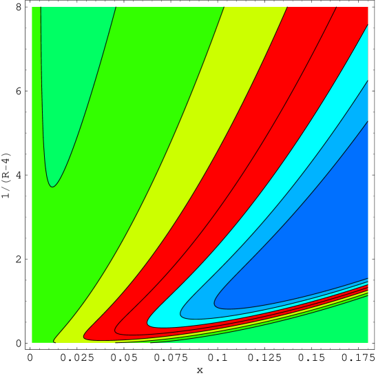
Figure 2: Contourplot for ${\tilde{n}}\equiv n-1$ as a function of the parameters $x$ and $(R-4)^{-1}$ (defined in (23)) in the model (22) for the mode that left the horizon $N_{k}=22$ e-folds before the end of inflation. The contours are (from outside to inside) for ${\tilde{n}}=-0.12,-0.09,-0.06,-0.03,0.00,+0.03,+0.06$, respectively. This means that the red region (between the contours $-0.06$ and $0.00$) corresponds with the $1\sigma$ WMAP constraint (3), while the yellow/green regions (near the axes) indicate values that are too low, and the blue regions values that are too high. The blue regions also correspond with a blue (${\tilde{n}}>0$) spectrum.

An important result that can be seen from the equations in the appendix, is that ${\tilde{\sigma}}_{\mathrm{H}}$ depends on the parameters $R$ and $x$ only. That means that the same is true for ${\tilde{n}}$. A contour plot of ${\tilde{n}}$ as a function of $x$ and $(R-4)^{-1}$ is given in figure 2 (we use $(R-4)^{-1}$ for the ordinate to avoid the curves getting squashed in the region $R\downarrow 4$). We conclude that there is a parameter region (the red area) where a spectral index compatible with the $1\sigma$ WMAP constraint (3) is produced. For $R<27/4$ (i.e. $(R-4)^{-1}>4/11$) it is even possible to get ${\tilde{n}}>0$ (the blue region). On the other hand, the amplitude does not just depend on $R$ and $x$, but also on $\alpha_{4}$ explicitly, as can be seen from (24).

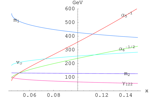
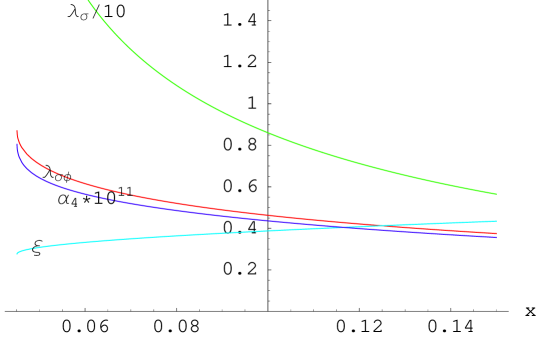
Figure 3: Variation of the dimensionful (top) and dimensionless (bottom) parameters in the model described in section 5.2 as a function of the one free parameter $x$ when all CMB (with ${\tilde{n}}=-0.03$) and SM constraints are applied (and choosing the smaller value for $R$).

Now we can apply all the constraints and determine the parameters in the following way. First we determine $x$ and $R$ from the spectral index constraint. Of course this cannot be done uniquely; basically we are free to choose e.g. $x$ (within certain limits as indicated in figure 2) and then $R$ is fixed by the constraint. Actually there are still two possibilities for $R$, but it turns out that the smaller value (corresponding to the upper branch in figure 2) leads to smaller non-renormalizable couplings $\alpha_{5}$ and $\alpha_{6}$, and also to a smaller dimensionless coupling $\lambda_{\sigma}$ (cf. (17)), which we consider more acceptable. Next $\alpha_{4}$ is fixed by the CMB amplitude constraint. Finally, the other parameters are determined by the coupling to the Higgs sector, in a way completely analogous to the treatment in sections 3.2 and 4. Setting ${\tilde{n}}=-0.03$, the central WMAP value, an explicit example with $x$ chosen to be $0.1$ is:

$$x=0.10:\quad R=4.32,\quad\alpha_{2}^{1/2}=1.30\times 10^{-15}\,\mbox{GeV},\quad\alpha_{4}=4.36\times 10^{-12},$$

$$\alpha_{5}^{-1}=357\,\mbox{GeV},\quad\alpha_{6}^{-1/2}=238\,\mbox{GeV},\quad\lambda_{\sigma\phi}=0.46,$$

$$\lambda_{\phi}=0.33,\quad\lambda_{\sigma}=8.6,\quad v_{\phi}=246\,\mbox{GeV},\quad v_{\sigma}=255\,\mbox{GeV},$$

$$m_{1}=427\,\mbox{GeV},\quad m_{2}=128\,\mbox{GeV},\quad\xi=0.39,\quad\gamma_{122}=65.5\,\mbox{GeV}.$$ (25)

For a more general picture see figure 3, where all the parameters have been plotted as a function of $x$ (and choosing the smaller value for $R$). We see that as $x$ increases, the non-renormalizable mass scales $\alpha_{5}^{-1}$ and $\alpha_{6}^{-1/2}$ also increase and that the (rather large) inflaton self-coupling $\lambda_{\sigma}$ decreases. Since smaller couplings are generically easier to deal with, the larger $x$ values would be favoured, but we shall not pursue this aspect further.

6 Loop corrections

Thus far we have assumed the potential $V$ to be an effective potential that approximately describes some extension of the SM, i.e. including all quantum effects. Nevertheless, since the calculation of the spectral index is based on the growth of quantum fluctuations during inflation, it is important to try to ascertain that the back-reaction of these fluctuations on the inflaton and on the SM is under control. After all, the $\sigma$ values vary over some twelve orders of magnitude from the inflationary to the electroweak domain. We therefore investigate in this section one-loop corrections based on $V$.

Corrections on the effective potential in the inflationary domain due to a Higgs loop have been investigated in [10], but not those coming from an inflaton loop. There is reason for concern, because the four-point self-coupling $\lambda_{\sigma}$ of the inflaton in the minimum of the potential, defined in (17), is rather large. For example, $\lambda_{\sigma}=8.6$ for the case (25). With such large couplings, computing loop ‘corrections’ is a hazardous endeavour and the calculations in this section are aimed at obtaining insight rather that getting quantitative results.

At strong couplings the non-perturbative phenomenon of ‘triviality’ comes into play: as the cut-off used to define the model is raised the renormalized couplings go down, and they even vanish in the infinite cut-off limit. Larger couplings imply a smaller maximum value of the cut-off, which is then interpreted as a momentum scale where the model breaks down (also known as ‘the Landau pole’). For a review of the application to the SM see [26, 29]. Assuming that this phenomenon applies also here, we shall tentatively use it to estimate the maximum cut-off from the large inflaton self-couplings.

Another reason for expecting such a scale where the model breaks down is the fact that it contains non-renormalizable couplings of dimension larger than four. This situation may be compared with effective pion models for QCD. These models are typically also non-renormalizable (even non-polynomial) and in the first instance only valid up to a few hundred MeV. Loop corrections may then further extend their validity. A well-developed scheme is chiral perturbation theory, in which all perturbative infinities are removed by counter-terms, with new physical constants parametrizing the corresponding finite parts [30, 31].

Before continuing in detail we should add the cautionary remark that the usual equilibrium effective potential can in principle not be applied blindly to systems out of equilibrium; we interpret it as being only indicative of the back-reaction. More sophisticated methods (e.g. Hartree or 2PI [32, 33]) are available, but they are a lot more complicated. In the inflationary domain the one-loop potential is complex due to the tree potential being unstable, and we shall concentrate on its real part.

Consider the potential

$$V^{(0)}=V_{0}-\frac{1}{2}\alpha_{2}\sigma^{2}+\frac{1}{4}\alpha_{4}\sigma^{4}-\frac{1}{5}\alpha_{5}\sigma^{5}+\frac{1}{6}\alpha_{6}\sigma^{6}-\frac{1}{2}\lambda_{\sigma\phi}\sigma^{2}\phi^{2}+\frac{1}{2}\mu^{2}\phi^{2}+\frac{1}{4}\lambda_{\phi}\phi^{4},$$ (26)

which is to be identified with $V$ at tree level. For simplicity we consider here only one real Higgs field to avoid the complications of massless Goldstone bosons, which would be absorbed by the W and Z bosons in the full SM. The one-loop contribution to the effective potential is given by (see e.g. [29])

$$V^{(1)}=\epsilon(m_{1}^{2})+\epsilon(m_{2}^{2})+{\rm c.t.}$$ (27)

where $\epsilon(m^{2})$ is the ground-state energy density of a free scalar field with mass $m$, c.t. denotes counter-terms and $m_{1}^{2}$ and $m_{2}^{2}$ are the eigenvalues

$$m_{1,2}^{2}=\frac{1}{2}\left(m_{\sigma}^{2}+m_{\phi}^{2}\pm\sqrt{(m_{\sigma}^{2}-m_{\phi}^{2})^{2}+4m_{\sigma\phi}^{4}}\right)$$ (28)

of the field-dependent mass matrix

$$m_{ab}^{2} = V_{,\,ab}^{(0)},\qquad(a,b)\in\{\sigma,\phi\},$$ (29)

$$m_{\sigma}^{2} \equiv m_{\sigma\sigma}^{2}=-\alpha_{2}+3\alpha_{4}\sigma^{2}-4\alpha_{5}\sigma^{3}+5\alpha_{6}\sigma^{4}-\lambda_{\sigma\phi}\phi^{2},$$ (30)

$$m_{\phi}^{2} \equiv m_{\phi\phi}^{2}=\mu^{2}-\lambda_{\sigma\phi}\sigma^{2}+3\lambda_{\phi}\phi^{2},\qquad m_{\sigma\phi}^{2}=-2\lambda_{\sigma\phi}\sigma\phi.$$ (31)

The ground-state energy density is given by

$$\epsilon(m^{2})=\int_{|{\bf p}|<\Lambda}\frac{d^{3}{\bf p}}{(2\pi)^{3}}\,\frac{1}{2}\sqrt{m^{2}+{\bf p}^{2}},$$ (32)

where we used a spherical cut-off $\Lambda$ on the three-momenta. Alternatively, we can use a four-dimensional Euclidean cut-off on the usual log-determinant form $\ln\det(m^{2}_{ab}+\partial^{2})$, which leads to

$$\epsilon(m^{2})=\frac{1}{2}\int_{|p|<\Lambda}\frac{d^{4}p}{(2\pi)^{4}}\,\ln(m^{2}+p^{2}).$$ (33)

The first regularization (32) has the advantage that time is kept real (and continuous), which is conceptually attractive for systems out of equilibrium, whereas the regularization (33) can be applied only in equilibrium with imaginary and somewhat fuzzy time. It turns out that both regularizations give very similar results and for definiteness we shall continue with the first one, (32).

Within the spirit of a polynomial parametrization, the counter-terms are supposed to be polynomial in $\sigma$ and $\phi$. It is desirable that they are able to cancel all divergencies as $\Lambda\rightarrow\infty$: the quartic ($\propto\Lambda^{4}$), quadratic ($\propto(m_{1}^{2}+m_{2}^{2})\Lambda^{2}$) and logarithmic ($\propto((m_{1}^{2})^{2}+(m_{2}^{2})^{2})\ln\Lambda$) ones. This is possible, since the square root in (28) drops out of the sum $m_{1}^{2}+m_{2}^{2}$, and also $(m_{1}^{2})^{2}+(m_{2}^{2})^{2}=(m_{\sigma}^{2})^{2}+(m_{\phi}^{2})^{2}+2(m_{\sigma\phi}^{2})^{2}$ is a polynomial in $\sigma$ and $\phi$. We define

$$\epsilon_{\mathrm{f}}(m^{2}) = \epsilon(m^{2})-\frac{1}{32\pi^{2}}\left(2\Lambda^{4}+2m^{2}\Lambda^{2}-(m^{2})^{2}\ln\frac{2e^{-1/4}\Lambda}{\nu}\right)$$ (34)

$$= \frac{1}{64\pi^{2}}\,(m^{2})^{2}\ln\frac{m^{2}}{\nu^{2}}+O(\Lambda^{-2}\ln\Lambda),$$ (35)

where we introduced the renormalization scale $\nu$. Dropping terms with negative powers of $\Lambda$, the form (33) for $\epsilon$ reduces also to the form (35) (with a different subtraction). We shall continue with the full form (34) with $\epsilon(m^{2})$ given in (32), without dropping negative powers of $\Lambda$.

The total potential at one loop is

$$V=V^{(0)}+V^{(1)}.$$ (36)

At this stage we have used counter-terms corresponding to all the terms in (26) to cancel the divergent cut-off dependence, as well as a few more: $\sigma^{7}$, $\sigma^{8}$, $\sigma^{3}\phi^{2}$ and $\sigma^{4}\phi^{2}$. The finite parts of these counter-terms have been assigned values by the subtraction in (34) (which is similar to the minimal subtraction used in perturbative QCD calculations). However, we still need at least some of these parameters to impose renormalization conditions on the potential. A minimal set of conditions is: ($i$) the real part of the expansion of $V$ in $\sigma$ around $\sigma=0$, at $\phi=0$, coincides with the original $V^{(0)}$ up to and including $\sigma^{5}$; ($ii$) $V$ vanishes in its absolute minimum at $\sigma=v_{\sigma}$, $\phi=v_{\phi}$; and ($iii$) $v_{\phi}=246$ GeV, unchanged. Requirement ($i$) expresses our wish to keep the potential unchanged in the inflationary domain, ($ii$) keeps the cosmological constant zero and ($iii$) is needed for electroweak phenomenology. Furthermore, in a sensible renormalized perturbation scheme it is desirable that the particle masses in loop diagrams are kept at the same values as in the tree graph starting point, so we add to our minimal set of conditions: ($iv$) $v_{\sigma}$, ($v$) $m_{\sigma}^{2}$ and ($vi$) $m_{\phi}^{2}$ are unchanged in the minimum of the potential. We can impose all these conditions by using only counter-terms according to the parameters listed in the tree potential (26). It turns out that $m_{\sigma\phi}^{2}$ ends up also very close to its tree value, so the particle masses $m_{1}$ and $m_{2}$ are indeed practically unchanged. The unusual combination of two classes of renormalization conditions, ($i$) in the inflationary region and ($ii$)–($vi$) in the ‘today’s physics’ region, makes an interesting problem.

Summarizing, the above renormalization conditions can be implemented by counter-terms of the form

$$\mbox{c.t.}=-\frac{1}{32\pi^{2}}\left[4\Lambda^{4}+2(m_{1}^{2}+m_{2}^{2})\Lambda^{2}-\left((m_{1}^{2})^{2}+(m_{2}^{2})^{2}\right)\ln\frac{2e^{-1/4}\Lambda}{\nu}\right]$$

$$\qquad\quad\mbox{}-\sum_{k=0}^{5}\mbox{Re}\left\{\frac{\partial^{k}}{\partial\sigma^{k}}\left[\epsilon_{\mathrm{f}}(m_{\sigma}^{2})+\epsilon_{\mathrm{f}}(m_{\phi}^{2})\right]\right\}_{\sigma=\phi=0}\frac{\sigma^{k}}{k!}$$ (37)

$$\qquad\quad\mbox{}+\delta\alpha_{6}\frac{\sigma^{6}}{6}-\delta\lambda_{\sigma\phi}\frac{\sigma^{2}\phi^{2}}{2}+\delta\mu^{2}\frac{\phi^{2}}{2}+\delta\lambda_{\phi}\frac{\phi^{4}}{4},$$

which satisfies condition ($i$) (note that $m_{1}^{2}=m_{\sigma}^{2}$ and $m_{2}^{2}=m_{\phi}^{2}$ in the inflationary region, since $\phi=0$). The first thing to check is the coefficient of the $\sigma^{6}$ term in the expansion around $\sigma=0$: it should not be large, as this might spoil the neglect of such a term in the inflationary domain. For the Higgs loop this has been done already in [10]. Its contribution to the coefficient of $\sigma^{6}/6$ is $-\lambda_{\sigma\phi}^{3}/(32\pi^{2}\mu^{2})$, which for the case (25) is only $-3.1\times 10^{-8}$ GeV^-2, even (much) smaller (in absolute value) than $\alpha_{6}=1.8\times 10^{-5}$ GeV^-2. For the inflaton loop the effects are even smaller because the effective mass $m_{\sigma}$ is tiny in the inflationary region; although $\ln(m_{\sigma}^{2}/\nu^{2})$ is the logarithm of a very small number, the $(m_{\sigma}^{2})^{2}$ in front of it makes it negligible. Since the terms with different powers of $\sigma$ up to and including $\sigma^{5}$ are by construction all approximately equal during inflation, a rough estimate of the relative importance of the inflaton loop corrections is given by $\alpha_{2}^{2}\ln(\alpha_{2}/\nu^{2})/(64\pi^{2}\alpha_{2}\sigma_{\mathrm{H}}^{2})={\mathcal{O}}(10^{-12})$.

We now impose the renormalization conditions ($ii$)–($vi$) in the minimum of the potential. These are five linear equations for the four parameters of the counter-terms in the third line of (37), plus the renormalization-scale parameter $\ln(\nu)$. Using as an example the parameter set (25) and choosing $\Lambda=\infty$ for a start, results in

$$\delta\alpha_{6}/\alpha_{6}=0.10,\quad\delta\lambda_{\sigma\phi}/\lambda_{\sigma\phi}=-0.011,\quad\delta\mu^{2}/\mu^{2}=-0.058,\quad\delta\lambda_{\phi}/\lambda_{\phi}=0.026,$$

$$\nu=939\,\mbox{GeV},\quad m_{\sigma\phi}^{2(0+1)}/m_{\sigma\phi}^{2(0)}=0.95,\quad\lambda_{\sigma}^{(0+1)}/\lambda_{\sigma}^{(0)}=2.07,$$ (38)

where (0) indicates the tree graph value and (0+1) the value derived from the full potential (36). The renormalization scale $\nu$ seems to be somewhat large, but small changes in $\ln(\nu)$ are of course amplified in $\nu$ itself. The finite counter-terms look reasonably small. The mixing mass $m_{\sigma\phi}$ is also close to the tree graph value, in accordance with our desire to keep the particle masses in the loop contributions close to the tree values. The inflaton self-coupling $\lambda_{\sigma}$ has increased by an unpleasant factor of about two, which seems to make the calculation untrustworthy. Another way of treating the renormalization to deal with this is discussed in appendix B.

Since we have removed the divergent cut-off dependence with the counter-terms, the renormalized effective potential cannot give us information on the scale where the model is expected to break down. For this we look at the bare coupling defined in terms of the bare potential $V^{(0)}+\mbox{c.t.}$, by

$$\lambda_{\sigma}^{(\rm b)}=(1/6)(V^{(0)}+\mbox{c.t.})_{,\,\sigma\sigma\sigma\sigma},$$ (39)

evaluated at its absolute minimum. In a simple $\phi^{4}$ model with one real scalar field the relation between the bare and renormalized coupling is qualitatively well described by the one-loop renormalization-group relation (see e.g. [29, 34])

$$\lambda^{(\rm b)}=\frac{\lambda}{1-\beta\lambda t}=\lambda+\lambda^{2}\beta t+\cdots,\qquad t=\ln(\Lambda/m)+{\rm constant},$$ (40)

with $\beta=9/(8\pi^{2})$ the one-loop beta-function coefficient. The bare coupling $\lambda^{(\rm b)}$ diverges when the denominator vanishes at the position of the ‘Landau pole’, and numerical simulations have indicated that this gives an order of magnitude estimate of the limiting $\Lambda$ (modulo the uncertainties related to methods of regularization and factors like $2e^{-1/4}$ in (34); for a review see e.g. [34]). As can be seen from the expansion in (40), the one-loop value of the bare coupling equals twice the tree value at the pole, and we shall use this for an estimate of the maximal cut-off $\Lambda_{\rm max}$:

$$\lambda_{\sigma}^{(\rm b)}/\lambda_{\sigma}=2\quad\Rightarrow\quad\Lambda=\Lambda_{\rm max}.$$ (41)

Using the results from the renormalization procedure in (38) we find that the maximum value is already reached near $\Lambda\simeq 600$ GeV, for which $\lambda_{\sigma}=12.8$ (and $\nu=702$ GeV).

The loop calculation in this section has given evidence that the flatness of the inflationary part of the potential can be kept consistent with quantum corrections. It appears that the model has to already break down at a fairly low scale. For the example (25) this could be around $700$ GeV or perhaps as low as $300$ GeV (see appendix B), but for larger $x$ values this scale slowly increases. Above this scale new physical input is needed.

7 Conclusion

In this paper we investigated the implications of the WMAP results for low-scale inflation and found that there are severe constraints. This is essentially because the proximity of the observed scalar spectral index ${\tilde{n}}\equiv n-1$ to zero is hard to reconcile with the small number of e-folds between horizon crossing of the observable scales and the end of inflation in these models. Working in the context of a phenomenological electroweak-scale inflation model that allows for tachyonic electroweak baryogenesis and consists of one additional scalar field $\sigma$ coupled to the Standard Model Higgs, we were led to further constraints on the inflaton–Higgs potential. However, we found that there is a range of parameters compatible with a spectral index close to (and even larger than) zero in this model.

The polynomial approximation together with all the constraints led to the conclusion that we need a $\sigma^{5}$ term in the potential during inflation (as in [10]). In addition $\sigma^{2}$ and $\sigma^{4}$ terms are needed, and (or instead of the $\sigma^{4}$) there might be a $\sigma^{3}$ term, but no powers higher than 5 can be present during inflation. The appearance of an odd power ($\sigma^{5}$) implies a local minimum at small negative values of the inflaton field ($\sigma=0$ being the value where the potential has a local maximum). A universe with initial conditions in this negative region would classically never stop inflating, which is why we assumed a small positive initial condition for the inflaton field. However, quantum tunnelling might very well make the case of a negative initial condition viable as well. The use of a polynomial approximation is quite natural for the inflationary region of the potential where the inflaton field is small, but it seems somewhat artificial in the large field region where the Higgs field comes into play. The odd and non-renormalizable power $\sigma^{5}$ in the potential appears to be the price we have to pay for keeping the number of parameters limited. It is not excluded of course that the model with its non-symmetric potential and non-renormalizable couplings can be embedded satisfactorily in a model with more symmetry that is also renormalizable, e.g. a supersymmetric extension of the Standard Model.

In the one-loop calculation we found that the very different renormalization conditions in the inflationary and electroweak regimes did not lead to unresolvable conflicts. In our results quantum corrections do not disrupt the required flatness of the potential in the inflationary region. The non-renormalizable couplings and also the relatively strong inflaton self-coupling suggest a breakdown of the model already occurring at a fairly low scale, perhaps below 1 TeV, depending on the choice of parameters.

We conclude with the important remark that the phenomenological model arrived at here can be falsified experimentally through its conspicuous generic feature: the existence of two (and only two) particle species with zero spin and masses around the electroweak scale, and couplings to the rest of the SM equal to that of the Higgs up to factors related to the mixing angle.

Appendix A Some analytical results for the full model with a quartic term

Starting from equations (22) and (23) in section 5.2, we find the following slow-roll field equation:

$$\mathrm{d}N=\frac{R}{x}\,\frac{\mathrm{d}{\tilde{\sigma}}}{R{\tilde{\sigma}}-3{\tilde{\sigma}}^{3}+{\tilde{\sigma}}^{4}}.$$ (42)

Integrating it from horizon crossing (subscript H) to the end of inflation (subscript e), we obtain for $R>4$ (with $N_{k}\equiv N_{\mathrm{e}}-N_{\mathrm{H}}$):

$$N_{k}=\frac{1}{3x}\Biggl{[}\frac{2+Q+2Q^{2}}{1+Q+Q^{2}}\ln\left(\frac{{\tilde{\sigma}}-1+Q+Q^{-1}}{\sqrt{{\tilde{\sigma}}^{2}-(2+Q+Q^{-1}){\tilde{\sigma}}+Q+Q^{-1}+Q^{2}+Q^{-2}}}\right)$$

$$+3\ln\left(\frac{{\tilde{\sigma}}}{{\tilde{\sigma}}-1+Q+Q^{-1}}\right)+\sqrt{3}\,\frac{Q(Q+1)}{Q^{3}-1}\,F({\tilde{\sigma}})\Biggr{]}^{{\tilde{\sigma}}={\tilde{\sigma}}_{\mathrm{e}}}_{{\tilde{\sigma}}={\tilde{\sigma}}_{\mathrm{H}}},$$ (43)

with

$$F({\tilde{\sigma}})\equiv\left\{\begin{array}[]{ll}\arctan\left(\frac{\frac{1}{2}\sqrt{3}(Q-Q^{-1})}{1+\frac{1}{2}Q+\frac{1}{2}Q^{-1}-{\tilde{\sigma}}}\right)&\mbox{for ${\tilde{\sigma}}<1+\frac{1}{2}Q+\frac{1}{2}Q^{-1}$}\\ \arctan\left(\frac{\frac{1}{2}\sqrt{3}(Q-Q^{-1})}{1+\frac{1}{2}Q+\frac{1}{2}Q^{-1}-{\tilde{\sigma}}}\right)+\pi&\mbox{for ${\tilde{\sigma}}>1+\frac{1}{2}Q+\frac{1}{2}Q^{-1}$}\end{array}\right.$$ (46)

and

$$Q^{3}\equiv\frac{1}{2}\left(R-2+\sqrt{R}\,\sqrt{R-4}\right)\qquad\Leftrightarrow\qquad R=2+Q^{3}+Q^{-3}.$$ (47)

The field value at the end of inflation that follows from the condition ${\tilde{\eta}}=1$ is for $x<1$ given by

$${\tilde{\sigma}}_{\mathrm{e}}=\frac{3}{4}\left(1+S+S^{-1}\right),\quad S^{3}\equiv\frac{8}{27}\left(R\,\frac{1-x}{x}+\frac{27}{8}-\sqrt{R\,\frac{1-x}{x}}\,\sqrt{R\,\frac{1-x}{x}+\frac{27}{4}}\right).$$ (48)

Appendix B Another renormalization treatment

We found in (38) that the already large inflaton self-coupling $\lambda_{\sigma}$ increased by another factor of two when applying the renormalization conditions. Of course, de facto, $\lambda_{\sigma}$ is a derived coupling: it depends on the other parameters of the model and we may just have to accept how it turns out. In principle, further experimental information is needed to be able to pin down the non-renormalizable couplings beyond $\alpha_{5}$ and $\alpha_{6}$, similar to what is done in chiral perturbation theory. To continue, we can pretend that our tree level values for couplings such as $\lambda_{\sigma}$ are actually phenomenologically correct, i.e. consider them as experimental input. Alternatively (but leading to the same treatment) we can work from the point of view presented at the end of section 4 that $\lambda_{\sigma}$ is a primary coupling and that the other parameters have to be chosen accordingly. (At this point we have assigned values to the non-renormalizable couplings of the $\sigma^{7}$, $\sigma^{8}$, $\sigma^{3}\phi^{2}$ and $\sigma^{4}\phi^{2}$ terms in a somewhat arbitrary way by the subtraction in (34) and the value of the renormalization scale $\nu$.) So we continue this exploration by imposing that in addition to $v_{\sigma}$, $v_{\phi}$ and the particle masses $m^{2}_{\sigma}$, $m^{2}_{\phi}$ and $m^{2}_{\sigma\phi}$, also the tree graph value of $\lambda_{\sigma}$ is to remain unchanged, and that the other parameters have to be chosen accordingly.

We add to our renormalization conditions: ($vii$) $m^{2}_{\sigma\phi}=m^{2(0)}_{\sigma\phi}$ and ($viii$) $\lambda_{\sigma}=\lambda_{\sigma}^{(0)}$. Since $\lambda_{\sigma}$ is naturally controlled by the $\alpha$ parameters, we add to (37) the finite counter-terms

$$+\,\delta\alpha_{7}\frac{\sigma^{7}}{7}+\delta\alpha_{8}\frac{\sigma^{8}}{8},$$ (49)

still keeping the coefficients of $\sigma^{3}\phi^{2}$ and $\sigma^{4}\phi^{2}$ set by the value of $\nu$. The result of this exercise is given by

$$\delta\alpha_{6}/\alpha_{6}=-0.75,\quad\delta\lambda_{\sigma\phi}/\lambda_{\sigma\phi}=0.15,\quad\delta\mu^{2}/\mu^{2}=0.34,\quad\delta\lambda_{\phi}/\lambda_{\phi}=0.092,$$

$$\nu=3987\,\mbox{GeV},\quad\delta\alpha_{7}^{-1/3}=217\,\mbox{GeV},\quad(-\delta\alpha_{8})^{-1/4}=363\,\mbox{GeV}.$$ (50)

We see that the scale of $\delta\alpha_{7}$ and $\delta\alpha_{8}$ is similar to that of $\alpha_{5}$ and $\alpha_{6}$, and the other counter-term parameters are larger than before in (38) but still reasonable, except that $\nu$ has slipped to a rather large value. We could fix $\nu$ to, say, 400 GeV and use one of the $\sigma^{k}\phi^{2}$ couplings in its place, but then the resulting counter-term parameters for the other couplings are larger. Moreover, we prefer to keep $\nu$ variable since it adjusts itself naturally in such a way that the loop correction vanishes as $\Lambda\rightarrow 0$.

When we try to determine the maximal cut-off in this case using the estimate (41), we find that this criterion cannot be applied meaningfully because the bare potential quickly becomes unstable (no lower bound) as $\Lambda$ is increased from zero. This happens already for $\Lambda$ between 200 and 300 GeV (where $\nu$ has come down to $\approx 300$ GeV). Such a low value is also suggested by the fact that $250$–$350$ GeV is the scale of the non-renormalizable couplings $\alpha_{5}$ and $\alpha_{6}$ in the example (25).

References

References

- [1] Spergel D N et al, First year WMAP observations: Determination of cosmological parameters, 2003 Astrophys. J. Suppl. 148 175 [astro-ph/0302209]
- [2] WMAP website: http://map.gsfc.nasa.gov
- [3] Peiris H V et al, First year WMAP observations: Implications for inflation, 2003 Astrophys. J. Suppl. 148 213 [astro-ph/0302225]
- [4] Kinney W H, Kolb E W, Melchiorri A and Riotto A, WMAPping inflationary physics, 2004 Phys. Rev.D 69 103516 [hep-ph/0305130]
- [5] Leach S M and Liddle A R, Constraining slow-roll inflation with WMAP and 2dF, 2003 Phys. Rev.D 68 123508 [astro-ph/0306305]
- [6] Rubakov V A and Shaposhnikov M E, Electroweak baryon number non-conservation in the early universe and in high energy collisions, 1996 Phys. Usp. 39 461 [hep-ph/9603208]
- [7] Krauss L M and Trodden M, Baryogenesis below the electroweak scale, 1999 Phys. Rev. Lett.83 1502 [hep-ph/9902420]
- [8] García-Bellido J, Grigoriev D, Kusenko A and Shaposhnikov M, Non-equilibrium electroweak baryogenesis from preheating after inflation, 1999 Phys. Rev.D 60 123504 [hep-ph/9902449]
- [9] Felder G et al, Dynamics of symmetry breaking and tachyonic preheating, 2001 Phys. Rev. Lett.87 011601 [hep-ph/0012142]
- [10] Copeland E J, Lyth D H, Rajantie A and Trodden M, Hybrid inflation and baryogenesis at the TeV scale, 2001 Phys. Rev.D 64 043506 [hep-ph/0103231]
- [11] García-Bellido J, Garcia-Pérez M and González-Arroyo A, Chern-Simons number production during preheating in hybrid inflation models, 2004 Phys. Rev.D 69 023504 [hep-ph/0304285]
- [12] Tranberg A and Smit J, Baryon asymmetry from electroweak tachyonic preheating, 2003 J. High Energy Phys. JHEP11(2003)016 [hep-ph/0310342]
- [13] Smit J, 2003 COSMO-03: Int. Workshop on Particle Physics and the Early Universe, transparencies at http://www.ippp.dur.ac.uk/cosmo03/BAUPT/smit.ps
- [14] Knox L and Turner M S, Inflation at the electroweak scale, 1993 Phys. Rev. Lett.70 371 [astro-ph/9209006]
- [15] Kinney W H and Mahanthappa K T, Inflation at low scales: General analysis and a detailed model, 1996 Phys. Rev.D 53 5455 [hep-ph/9512241]
- [16] German G, Ross G and Sarkar S, Low-scale inflation, 2001 Nucl. Phys.B 608 423 [hep-ph/0103243]
- [17] Lyth D H, Which is the best inflation model?, 2003 Preprint hep-th/0311040
- [18] Shafi Q and Vilenkin A, Inflation with SU(5), 1984 Phys. Rev. Lett.52 691
- [19] Linde A D, Hybrid inflation, 1994 Phys. Rev.D 49 748 [astro-ph/9307002]
- [20] Liddle A R and Lyth D H, The cold dark matter density perturbation, 1993 Phys. Rep. 231 1 [astro-ph/9303019]
- [21] Dodelson S and Hui L, A horizon ratio bound for inflationary fluctuations, 2003 Phys. Rev. Lett.91 131301 [astro-ph/0305113]
- [22] Liddle A R and Leach S M, How long before the end of inflation were observable perturbations produced?, 2003 Phys. Rev.D 68 103503 [astro-ph/0305263]
- [23] Skullerud J-I, Smit J and Tranberg A, W and Higgs particle distributions during electroweak tachyonic preheating, 2003 J. High Energy Phys. JHEP08(2003)045 [hep-ph/0307094]
- [24] Csikor F, Fodor Z and Heitger J, Endpoint of the hot electroweak phase transition, 1999 Phys. Rev. Lett.82 21 [hep-ph/9809291]
- [25] Van Tent B J W, Multiple-field inflation and the CMB, 2004 Class. Quantum Grav.21 349 [astro-ph/0307048]
- [26] Hagiwara K et al, Review of particle physics, 2002 Phys. Rev.D 66 010001
- [27] García-Bellido J, Garcia-Pérez M and González-Arroyo A, Symmetry breaking and false vacuum decay after hybrid inflation, 2003 Phys. Rev.D 67 103501 [hep-ph/0208228]
- [28] De Wit B and Smith J, 1986 Field Theory in Particle Physics vol 1 (Amsterdam: North-Holland)
- [29] Sher M, Electroweak Higgs potentials and vacuum stability, 1989 Phys. Rep. 179 273
- [30] Gasser J and Leutwyler H, Chiral perturbation theory to one loop, 1984 Annals Phys. 158 142
- [31] Weinberg S, 1996 The Quantum Theory of Fields (Cambridge: Cambridge University Press) sections 12.3 and 19.5
- [32] Cormier D and Holman R, Spinodal decomposition and inflation: dynamics and metric perturbations, 2000 Phys. Rev.D 62 023520 [hep-ph/9912483]
- [33] Berges J and Serreau J, Progress in nonequilibrium quantum field theory, 2003 Preprint hep-ph/0302210
- [34] Heller U M, Status of the Higgs mass bound, 1994 Nucl. Phys. Proc. Suppl. 34 101 [hep-lat/9311058]