We present an updated analysis of the rare decay $K_{L}\rightarrow\pi^{0}\mu^{+}\mu^{-}$ within the Standard Model. In particular, we present the first complete calculation of the two-photon CP-conserving amplitude within Chiral Perturbation Theory, at the lowest non-trivial order. Our results confirm previous findings that the CP-conserving contribution to the decay rate cannot be neglected. By means of an explicit two-loop calculation, we show that this contribution can be estimated with sufficient accuracy compared to the CP-violating terms. We predict $\mathcal{B}(K_{L}\rightarrow\pi^{0}\mu^{+}\mu^{-})_{\mathrm{SM}}=(1.5\pm 0.3)\times 10^{-11}$, with approximately equal contributions from the CP-conserving component, the indirect-CP-violating term, and the interesting direct-CP-violating amplitude. The error of this prediction is mainly of parametric nature and could be substantially reduced with better data on the $K_{S}\rightarrow\pi^{0}\ell^{+}\ell^{-}$ modes. The Standard Model predictions for various differential distributions and the sensitivity to possible new-physics effects are also briefly discussed.

1 Introduction

The rare decays $K_{L}\rightarrow\pi^{0}\ell^{+}\ell^{-}$ are among the most interesting channels for precision studies of CP violation and flavour mixing in the $\Delta S=1$ sector [1]. The decay amplitudes of these processes have three main ingredients: i. a clean direct-CP-violating component determined by short-distance dynamics; ii. an indirect-CP-violating (CPV) term due to $K_{L}$-$K_{S}$ mixing; iii. a long-distance CP-conserving (CPC) component due to two-photon intermediate states. Although generated by very different dynamics, these three components are of comparable size within the Standard Model (SM). The precise knowledge about their magnitude (particularly of ii. and iii.) has substantially improved in the recent past [2]. This improvement has been made possible by the observation of the $K_{S}\rightarrow\pi^{0}\ell^{+}\ell^{-}$ decays [3, 4] and also by precise experimental studies of the $K_{L}\rightarrow\pi^{0}\gamma\gamma$ diphoton spectrum [5, 6].

The main difference of the $K_{L}\rightarrow\pi^{0}\mu^{+}\mu^{-}$ mode with respect to the electron channel, which has recently been re-analysed in Ref. [2], is the two-photon CPC contribution. The latter corresponds to transitions into final states where the lepton pair has $J^{\mathrm{CP}}=0^{++}$ or $2^{++}$. The $J^{\mathrm{CP}}=0^{++}$ case can safely be neglected in the electron mode, because of the strong helicity suppression [7, 8, 9]. On the contrary, the $K_{L}\rightarrow\pi^{0}(\gamma\gamma)_{J=0}\rightarrow\pi^{0}(\ell^{+}\ell^{-})_{J=0}$ amplitude generates the by far dominant CPC contribution in the muon mode [8, 10]. The main purpose of the present paper is a detailed analysis of this CPC amplitude, which is a fundamental ingredient to obtain a reliable SM prediction for the entire $K_{L}\rightarrow\pi^{0}\mu^{+}\mu^{-}$ decay width.

Chiral Perturbation Theory (CHPT) provides a natural framework to analyse the CP-conserving $K_{L}\rightarrow\pi^{0}\mu^{+}\mu^{-}$ amplitude. Here the first non-trivial contribution arises at $\mathcal{O}(p^{4})$ from two-loop diagrams of the type $K_{L}\rightarrow\pi^{0}(P^{+}P^{-})\rightarrow\pi^{0}(\gamma\gamma)\rightarrow\pi^{0}\mu^{+}\mu^{-}$, where $P=\pi,K$. This structure is very similar to the two-loop $K_{S}\rightarrow\mu^{+}\mu^{-}$ amplitude analysed by Ecker and Pich [11]: there are no counterterms at $\mathcal{O}(p^{4})$ and the sum of all loop diagrams yields a finite unambiguous result. The $K_{S}\rightarrow\mu^{+}\mu^{-}$ amplitude of Ref. [11] has indeed been used by Heiliger and Sehgal [10] to estimate the dominant pion-loop terms in $K_{L}\rightarrow\pi^{0}\mu^{+}\mu^{-}$. These authors extracted from the $K_{S}\rightarrow\mu^{+}\mu^{-}$ amplitude an appropriate electromagnetic form factor, describing the $(\pi^{+}\pi^{-})_{J=0}\rightarrow(\gamma\gamma)\rightarrow\mu^{+}\mu^{-}$ transition, and used it in conjunction with a constant $K_{L}\rightarrow 3\pi$ vertex to estimate the $K_{L}\rightarrow\pi^{0}\mu^{+}\mu^{-}$ amplitude. Although quite reasonable from a phenomenological point of view, this result is not fully justified within CHPT.

By means of an explicit two-loop calculation, we show that the factorization of the electromagnetic form factor holds exactly at $\mathcal{O}(p^{4})$, independently of the structure of the $K_{L}\rightarrow 3\pi$ amplitude, and independently of the nature of the charged pseudoscalar meson inside the loop. We are then able to present the first complete $\mathcal{O}(p^{4})$ estimate of the CPC $K_{L}\rightarrow\pi^{0}\mu^{+}\mu^{-}$ amplitude, with the correct chiral dynamics of the $K_{L}\rightarrow 3\pi$ vertex and the missing kaon-loop contribution. In order to check the stability of this result, we also performed a detailed study of possible higher-order contributions, taking into account the recent experimental information on the $K_{L}\rightarrow\pi^{0}\gamma\gamma$ decay distribution. The main outcome of this analysis is a reliable theoretical estimate of the ratio

$$R_{\gamma\gamma}=\frac{\Gamma(K_{L}\rightarrow\pi^{0}\ell^{+}\ell^{-})_{\rm CPC}}{\Gamma(K_{L}\rightarrow\pi^{0}\gamma\gamma)}~{}.$$ (1)

Despite numerator and denominator receive, separately, large corrections beyond $\mathcal{O}(p^{4})$, $R_{\gamma\gamma}$ turns out to be a rather stable quantity, with a theoretical error conservatively estimated to be around $30\%$.

Combining the analysis of the CPC amplitude with an updated estimate of the CPV terms, we finally arrive to the prediction $\mathcal{B}(K_{L}\rightarrow\pi^{0}\mu^{+}\mu^{-})_{\mathrm{SM}}\approx 1.5\times 10^{-11}$ for the total branching ratio. This turns out to be composed by almost equal amounts of CPC, indirect-CPV and direct-CPV (including the interference) terms. The present error of this estimate is around $30\%$, but it is largely dominated by the parametric uncertainty due to the $\mathcal{B}(K_{S}\rightarrow\pi^{0}\ell^{+}\ell^{-})$ measurements. The irreducible theoretical uncertainty is around $10\%$ and can be further decreased by suitable kinematical cuts. We thus conclude that the $K_{L}\rightarrow\pi^{0}\mu^{+}\mu^{-}$ channel is a very promising mode for future precision studies of CP violation in the $\Delta S=1$ sector, with complementary virtues and disadvantages with respect to the other golden modes, namely $K_{L}\rightarrow\pi^{0}\nu\bar{\nu}$ and $K_{L}\rightarrow\pi^{0}e^{+}e^{-}$. As an illustrative example of the discovery potential of the two $K_{L}\rightarrow\pi^{0}\ell^{+}\ell^{-}$ channels, we conclude our analysis showing that – even with the present parametric uncertainties – these two modes would yield a clear non-standard signature for the new-physics scenario recently proposed in Ref. [12].

The paper is organized as follows: in Section 2 we discuss the kinematics and the general amplitude decomposition of $K_{L}\rightarrow\pi^{0}\ell^{+}\ell^{-}$ decays. In Section 3 we update the prediction of the CP-violating rate for the muon mode. Section 4 contains the main results of this work, namely the analytical and numerical study of the $K_{L}\rightarrow\pi^{0}(\ell^{+}\ell^{-})_{J=0}$ CP-conserving amplitude. The phenomenological analysis of $K_{L}\rightarrow\pi^{0}\mu^{+}\mu^{-}$ decays, within and beyond the SM, is presented in Section 5. The results are summarized in the Conclusions.

2 Amplitude decomposition and differential distributions

The most general decomposition of the $K_{L}\rightarrow\pi^{0}\ell^{+}\ell^{-}$ amplitude involves four independent form factors ($S$, $P$, $V$, and $A$) [13]:

$$\mathcal{A}(K_{L}\rightarrow\pi^{0}\ell^{+}\ell^{-})=\frac{e^{2}G_{F}}{(4\pi)^{2}}\Big{[}m_{\ell}\bar{u}(p)v(p^{\prime})S(z,\tilde{y})+m_{\ell}\bar{u}(p)\gamma_{5}v(p^{\prime})P(z,\tilde{y})$$

$$\quad\qquad+(p_{K}+p_{\pi})_{\mu}\bar{u}(p)\gamma^{\mu}v(p^{\prime})V(z,\tilde{y})+(p_{K}+p_{\pi})_{\mu}\bar{u}(p)\gamma^{\mu}\gamma_{5}v(p^{\prime})A(z,\tilde{y})\Big{]}~{}.\qquad$$ (2)

The two independent kinematical variables can be chosen as

$$z=\frac{(p+p^{\prime})^{2}}{m_{K}^{2}}~{},\qquad\tilde{y}=\frac{2}{m_{K}^{2}}\frac{p_{K}\!\cdot\!(p-p^{\prime})}{\beta_{\pi}(z)\beta_{\ell}(z)}~{},\qquad$$ (3)

where

$$r_{i}=\frac{m_{i}}{m_{K}}~{},\quad\beta_{\ell}(z)=\left(1-\frac{4r_{\ell}^{2}}{z}\right)^{1/2},\quad\beta_{\pi}(z)=\left(1+r_{\pi}^{4}+z^{2}-2z-2r_{\pi}^{2}-2zr_{\pi}^{2}\right)^{1/2}.\$$ (4)

The variable $\tilde{y}$ coincides with $\cos\theta_{\ell}$, where $\theta_{\ell}$ is the angle between $K_{L}$ and $\ell^{-}$ spatial momenta in the dilepton center-of-mass frame, and the two independent ranges are

$$4r_{\ell}^{2}\leq z\leq(1-r_{\pi})^{2}~{},\qquad-1<{\tilde{y}}\equiv\cos\theta_{\ell}<1~{},$$ (5)

With these conventions, the general expression of the differential decay rate is

$$\frac{d^{2}\Gamma}{dzd\tilde{y}}~{}=~{}\frac{\alpha^{2}G_{F}^{2}m_{K}^{5}\beta_{\pi}(z)\beta_{\ell}(z)}{2^{12}\pi^{5}}\Big{\{}r_{\ell}^{2}\beta_{\ell}^{2}(z)z|S(z,\tilde{y})|^{2}+r_{\ell}^{2}z|P(z,\tilde{y})|^{2}$$

$$\qquad\quad+\beta_{\pi}^{2}(z)(1-\beta_{\ell}^{2}\tilde{y}^{2})|V(z,\tilde{y})|^{2}+\left[\beta_{\pi}^{2}(z)(1-\beta_{\ell}^{2}\tilde{y}^{2})+4r_{\ell}^{2}(2+2r_{\pi}^{2}-z)\right]|A(z,\tilde{y})|^{2}$$

$$\qquad\quad+4r_{\ell}^{2}(1-r_{\pi}^{2})\mathrm{Re}\left[A(z,\tilde{y})^{\ast}P(z,\tilde{y})\right]+4r_{\ell}^{2}\beta_{\pi}(z)\beta_{\ell}(z)\tilde{y}\mathrm{Re}\left[V(z,\tilde{y})^{\ast}S(z,\tilde{y})\right]\Big{\}}.\qquad$$ (6)

The $\tilde{y}$ variable is CP-odd and leads to a strong kinematical suppression. For this reason, it is convenient to expand the four form factors in a multipole series:

$$F(z,\tilde{y})=F_{0}(z)+\tilde{y}F_{1}(z)+\ldots\qquad F=S,P,V,A~{}.$$ (7)

The CP properties of the amplitudes are the following: the odd multipoles of $S$ and the even multipoles of $P$, $V$ and $A$, vanish in the limit of exact CP invariance. All short-distance contributions to the higher multipoles are negligible, since they cannot be generated by dimension-six operators. To a good approximation, we can also neglect all the long-distance contributions generated by two-photon amplitudes in the CPV multipoles. As a result, we are left with five potentially interesting terms:

$A_{0},P_{0}$

: direct CPV amplitudes of short-distance origin;

$V_{0}$

: CPV amplitude which receives both short-distance (direct CPV component) and long-distance (indirect CPV component) contributions [14, 15];

$S_{0},V_{1}$

: CPC amplitude induced by the long-distance transition $K_{L}\rightarrow\pi^{0}(\gamma\gamma)_{J=0,2}\rightarrow\pi^{0}\ell^{+}\ell^{-}$; with the $J^{\mathrm{PC}}=0^{++}$ two-photon state contributing only to $S_{0}$.

As mentioned in the Introduction, these amplitudes turn out to be of comparable magnitude despite they are generated by very different dynamical mechanisms. Given the normalization in Eq. (2), the CPV short-distance multipoles are of $\mathcal{O}(\mathrm{Im}(V_{ts}^{*}V_{td})/e^{2}\sim 10^{-3})$ within the SM, $V^{\mathrm{ind}}_{0}$ is of $\mathcal{O}(\varepsilon\sim 10^{-3})$ and the two-photon CPC terms are of $\mathcal{O}(\alpha/(4\pi)\sim 10^{-3})$. We stress that these five multipoles are the only interesting terms also beyond the SM, and that only the short-distance terms ($A_{0}$, $P_{0}$, $V^{\mathrm{dir}}_{0}$) could receive sizable non-standard contributions.

The differential $z$ distribution taking into account only the five potentially interesting terms can be written as

$$\frac{d\Gamma}{dz}=\frac{d\Gamma_{\mathrm{CPC}}}{dz}+\frac{d\Gamma_{\mathrm{CPV}}}{dz}~{},$$ (8)

where

$$\frac{d\Gamma_{\mathrm{CPC}}}{dz} =\frac{\alpha^{2}G_{F}^{2}m_{K}^{5}\beta_{\pi}(z)\beta_{\ell}(z)}{2^{11}\pi^{5}}\left\{r_{\ell}^{2}\beta_{\ell}^{2}(z)z|S_{0}(z)|^{2}+\frac{2}{15}\beta_{\pi}^{2}(z)\left(1+\frac{6r_{\ell}^{2}}{z}\right)|V_{1}(z)|^{2}\right.$$

$$\left.\qquad\qquad+\frac{4}{3}r_{\ell}^{2}\beta_{\pi}(z)\beta_{\ell}(z)\mathrm{Re}[S_{0}(z)V_{1}(z)^{\ast}]\right\},\qquad$$ (9)

$$\frac{d\Gamma_{\mathrm{CPV}}}{dz} =\frac{\alpha^{2}G_{F}^{2}m_{K}^{5}\beta_{\pi}(z)\beta_{\ell}(z)}{2^{11}\pi^{5}}\left\{r_{\ell}^{2}z|P_{0}(z)|^{2}+\frac{2}{3}\beta_{\pi}^{2}(z)\left(1+\frac{2r_{\ell}^{2}}{z}\right)|V_{0}(z)|^{2}\right.$$

$$\qquad\qquad+\left[\frac{2}{3}\beta_{\pi}^{2}(z)\left(1+\frac{2r_{\ell}^{2}}{z}\right)+4r_{\ell}^{2}(2+2r_{\pi}^{2}-z)\right]|A_{0}(z)|^{2}$$

$$\left.\qquad\qquad+4r_{\ell}^{2}(1-r_{\pi}^{2})\mathrm{Re}\left[A_{0}(z)^{\ast}P_{0}(z)\right]\frac{{}}{{}}\right\}~{}.$$ (10)

The asymmetric integration on $\tilde{y}$ give rise to the following CPV distribution

$$\frac{dA_{\mathrm{FB}}}{dz} = \int d\tilde{y}~{}\frac{d^{2}\Gamma}{dzd\tilde{y}}~{}\mathrm{sgn(\tilde{y})}~{}=~{}\frac{\alpha^{2}G_{F}^{2}m_{K}^{5}\beta_{\pi}^{2}(z)\beta_{\ell}(z)}{2^{12}\pi^{5}}$$ (11)

$$\times\mathrm{Re}\left[V_{0}(z)^{\ast}\left(4r_{\ell}^{2}\beta_{\ell}(z)S_{0}(z)+\beta_{\pi}(z)\left(1+\frac{4r_{\ell}^{2}}{z}\right)V_{1}(z)\right)\right]~{}.$$

With a proper normalization, $A_{\mathrm{FB}}$ can be identified with the forward-backward or the energy asymmetry of the two leptons.

3 The CP-violating rate

An updated discussion of the CP-violating amplitude for the electron case ($\ell=e$) can be found in Ref. [2], to which we refer for more details. Most of the ingredients of this analysis can easily be transferred to the muon case. Following the notation of Ref. [2, 15], the dominant indirect-CPV amplitude leads to

$$V_{0}^{\mathrm{ind}}(z)=\pm\varepsilon\left[a_{S}+b_{S}z+\frac{W_{S}^{\pi\pi}(z)}{G_{F}m_{K}^{2}}\right]\approx\pm\varepsilon(a_{S}+b_{S}z)~{},$$ (12)

where the $\pm$ refers to the relative sign between this long-distance term and the short-distance (direct-CPV) component of the vector amplitude. The latter is given by

$$V_{0}^{\mathrm{dir}}(z)=i\frac{4\pi y_{7V}}{\sqrt{2}\alpha}f_{+}(z)\mathrm{\operatorname{Im}}\lambda_{t}~{},$$ (13)

where, as usual, $\lambda_{t}$ denotes the CKM combination $V_{ts}^{\ast}V_{td}$, $f_{\pm}(z)$ are the $K\rightarrow\pi$ form factors of the $\bar{s}\gamma^{\mu}d$ current, and $y_{7V,A}$ are the Wilson coefficients of the leading flavour-changing neutral-current (FCNC) operators [16]. Similarly, the axial-current operator leads to the clean short-distance terms

$$A_{0}(z) =i\frac{4\pi y_{7A}}{\sqrt{2}\alpha}f_{+}(z)\mathrm{\operatorname{Im}}\lambda_{t}~{},$$ (14)

$$P_{0}(z) =-i\frac{8\pi y_{7A}}{\sqrt{2}\alpha}f_{-}(z)\mathrm{\operatorname{Im}}\lambda_{t}~{}.$$ (15)

Note that, contrary to the electron case, here the pseudoscalar amplitude is not helicity suppressed (see Eq. (10)).

Thanks to the recent NA48 results,

$${\cal B}(K_{S}\rightarrow\pi^{0}e^{+}e^{-})_{m_{ee}>165~{}\mathrm{MeV}} =\left(3.0_{-1.2}^{+1.5}\pm 0.2\right)\times 10^{-9}~{}\cite[cite]{[\@@bibref{}{NA48ee}{}{}]}~{},$$ (16)

$${\cal B}(K_{S}\rightarrow\pi^{0}\mu^{+}\mu^{-}) =\left(2.9_{-1.2}^{+1.4}\pm 0.2\right)\times 10^{-9}~{}\cite[cite]{[\@@bibref{}{NA48mm}{}{}]}~{},$$ (17)

the large theoretical uncertainty about the size of the indirect-CPV amplitude has been strongly reduced. Under the natural and mild assumption that the form factor of the $K_{S}\rightarrow\pi^{0}\ell^{+}\ell^{-}$ amplitude is equal to $f_{+}(z)$, i.e. assuming $(b_{S}/a_{S})z=f_{+}(z)-1=0.39z$ [15], the combination of these two measurements leads to

$$|a_{S}|=1.2\pm 0.2~{}.$$ (18)

Within the SM, the main parametric uncertainty on the direct-CPV amplitude is due to $\mathrm{Im}\lambda_{t}$. According to recent global CKM fits [17]:

$$\mathrm{\operatorname{Im}}\lambda_{t}=\mathrm{\operatorname{Im}}(V_{ts}^{\ast}V_{td})\overset{{}_{\mathrm{SM}}}{\longrightarrow}(1.36\pm 0.12)\times 10^{-4}~{}.$$ (19)

Keeping the explicit dependence on these two main input values, and combining all the CPV contributions, we obtain the following phenomenological expression:

$${\cal B}(K_{L}\rightarrow\pi^{0}\mu^{+}\mu^{-})_{\mathrm{CPV}}\,=\,10^{-12}\times\left[3.7|a_{S}|^{2}\pm 1.6|a_{S}|\left(\frac{\displaystyle\mathrm{\operatorname{Im}}\lambda_{t}}{\displaystyle 10^{-4}}\right)+1.0\left(\frac{\displaystyle\mathrm{\operatorname{Im}}\lambda_{t}}{\displaystyle 10^{-4}}\right)^{2}\right]~{}.$$ (20)

The numerical coefficients have been obtained setting $y_{7A}=-(0.68\pm 0.03)\alpha(M_{Z})$ and $y_{7V}=(0.73\pm 0.04)\alpha(M_{Z})$, corresponding to ${\overline{m}}_{t}(m_{t})=167\pm 5$ GeV and a renormalization scale between $0.8$ and $1.2$ GeV [16]. Using these inputs, the error on each of the three coefficients in Eq. (20) is below $10\%$. The result depends very mildly on $f_{-}$, which has been set to $f_{-}(z)=-0.14$; however, the relative weight of the three terms in (20) is different with respect to the electron case. This happens because of the $r_{\ell}$ terms in Eq. (10), which enhance the axial-current direct-CPV contribution. As discussed in Ref. [2], the preferred theoretical choice for the sign of the interference term is the positive sign. The same conclusion has recently been reached also by Friot, Greynat and de Rafael, who reinforced this theoretical argument with a detailed dynamical analysis of $K\to\pi\gamma\to\pi\ell^{+}\ell^{-}$ amplitudes in the large $N_{C}$ limit [18].

4 The CP-conserving rate

As discussed in the Introduction, the leading CHPT contribution to the CP-conserving $K_{L}\rightarrow\pi^{0}\ell^{+}\ell^{-}$ amplitude is generated by two-loop diagrams of $\mathcal{O}(e^{4}p^{4})$. The general structure of these diagrams is indicated in Fig. 2–2. Due to the absence of local contributions, the complete two-loop amplitude of $\mathcal{O}(e^{4}p^{4})$ is finite and does not depend on unknown coefficients.

4.1 General decomposition of the loop amplitude

From the general structure in Fig. 2, we can decompose the CPC amplitude as

$$\mathcal{A}(K_{L}\rightarrow\pi^{0}\ell^{+}\ell^{-})_{\mathrm{CPC}}=\frac{ie^{2}}{2}\int\frac{d^{d}q^{\prime}}{(2\pi)^{d}}~{}A_{\gamma\gamma}^{\mu\nu}(p^{\prime}-q^{\prime},p+q^{\prime})~{}L_{\mu\nu}(p,p^{\prime};q^{\prime})~{},$$ (21)

where

$$L^{\mu\nu}(p,p^{\prime};q^{\prime})=\bar{u}(p)\left[\gamma^{\nu}\frac{1}{-q^{\prime}\!\!\!\!/-m_{\ell}}\gamma^{\mu}+\gamma^{\mu}\frac{1}{q^{\prime}\!\!\!\!/+p\!\!\!/-p^{\prime}\!\!\!\!/-m_{\ell}}\gamma^{\nu}\right]v(p^{\prime})$$ (22)

and $A_{\gamma\gamma}^{\mu\nu}$ is defined by the $K_{L}\rightarrow\pi^{0}\gamma\gamma$ amplitude with off-shell photons:

$$\mathcal{A}[K_{L}\rightarrow\pi^{0}\gamma(\epsilon_{1},t)\gamma(\epsilon_{2},k)]=A_{\gamma\gamma}^{\mu\nu}(t,k)\epsilon_{1}^{\nu}\epsilon_{2}^{\mu}~{}.$$ (23)

A strong simplification arises by the observation that the leptonic tensor obeys the Ward-identity relations

$$t_{\nu}L^{\mu\nu}=k_{\mu}L^{\mu\nu}=0~{}.$$ (24)

This implies that we can neglect in $A_{\gamma\gamma}^{\mu\nu}$ all the manifestly off-shell terms of the type $t^{\mu}t^{\nu}$, $k^{\mu}t^{\nu}$, $k^{\mu}k^{\nu}$. The non-trivial Lorentz structure of $A_{\gamma\gamma}^{\mu\nu}$ is then identical to the one of the on-shell amplitude [19, 20] and its calculation proceeds in a very similar way.

         

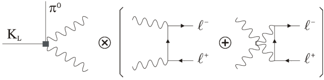
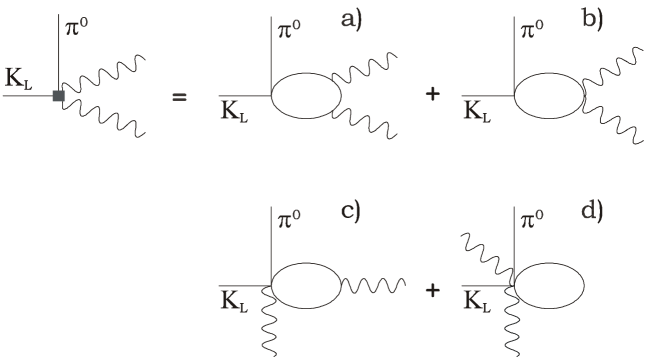
Figure 1: General decomposition of the $K_{L}\rightarrow\pi^{0}\ell^{+}\ell^{-}$ amplitude.

         

Figure 2: Lowest-order diagrams contributing to the $K_{L}\rightarrow\pi^{0}\gamma\gamma$ amplitude in the basis of Ref. [19].

As shown in Ref. [19], employing a suitable basis for the pseudoscalar meson fields, it is possible to reduce the number of independent diagrams contributing to the $K_{L}\rightarrow\pi^{0}\gamma\gamma$ amplitude to the four terms in Fig. 2. We note here that this structure can be further simplified with a suitable decomposition of the $K\rightarrow\pi^{0}P^{+}P^{-}$ amplitude, which acts as an effective vertex in the diagrams 2a–2b. At $\mathcal{O}(p^{2})$ we can write:

$$\mathcal{A}[K\rightarrow\pi^{0}P^{+}(p_{+})P^{-}(p_{-})]=i\left[a_{0}+a_{1}z+a_{2}(p_{+}^{2}+p_{-}^{2}-2m_{P}^{2})\right]~{},$$ (25)

where $z$ is defined as in Eq. (3) and the $a_{i}$ do not depend on the meson momenta. At this order gauge invariance forces the effective vertices of the diagrams 2c–2d to be completely determined by Eq. (25) via the minimal substitution. It is then easy to realize that the complete sum of the four terms in Fig. 2 is equivalent to the sum of 2a–2b performed without the off-shell term $a_{2}$. We are therefore left with the calculation of only two irreducible diagrams, with an effective $K\rightarrow\pi^{0}P^{+}P^{-}$ vertex which does not depend on the loop momenta:

$$M_{\pi^{0}PP}^{(2)}(z)=a_{0}+a_{1}z~{}.$$ (26)

This re-organization of the calculation leads to several advantages: i) a reduction of the number of relevant diagrams; ii) a manifest link with the $K_{S}\rightarrow\ell^{+}\ell^{-}$ calculation of Ref. [11]; iii) the possibility to include a well-defined class of higher-order contributions (see e.g. Ref. [21]). As we shall show later on, the latter step is achieved in the case of the dominant pion loops by the replacement of $M_{3\pi}^{(2)}(z)$ with the $K\rightarrow\pi^{0}\pi^{+}\pi^{-}$ amplitude determined by experiments.

The explicit integration over the $P$-meson loop in $A^{\mu\nu}_{\gamma\gamma}$, namely

$$A^{\mu\nu}_{\gamma\gamma}(p^{\prime}-q^{\prime},p+q^{\prime})^{(P)}=-e^{2}M^{(2)}_{\pi^{0}PP}(z)\int\frac{d^{d}q}{(2\pi)^{d}}\frac{(2q-k)^{\mu}(2q+t)^{\nu}-g^{\mu\nu}(q^{2}-m_{P}^{2})}{[(q+t)^{2}-m_{P}^{2}][(q-k)^{2}-m_{P}^{2}][q^{2}-m_{P}^{2}]}~{},$$

leads to

$$\mathcal{A}(K_{L}\to\pi^{0}\ell^{+}\ell^{-})_{\mathrm{CPC}}^{(P)}=-\frac{e^{4}}{16\pi^{2}}M^{(2)}_{\pi^{0}PP}(z)$$

$$\qquad\times\int_{0}^{1}dx\int_{0}^{1-x}dy\int\frac{d^{d}q^{\prime}}{(2\pi)^{d}}\frac{u(p)\gamma^{\nu}(-q^{\prime}\!\!\!\!/-m_{\ell})\gamma^{\mu}v(p^{\prime})}{[(q^{\prime})^{2}-m^{2}_{\ell}](q^{\prime}+p)^{2}(q^{\prime}-p^{\prime})^{2}}$$

$$\qquad\times\left[\frac{4xy}{\Delta(x,y)}t_{\mu}k_{\nu}+\frac{-2xy(zm_{K}^{2}-t^{2}-k^{2})+y(2y-1)t^{2}+x(2x-1)k^{2}}{\Delta(x,y)}g_{\mu\nu}\right]~{},\qquad$$ (27)

where

$$\Delta(x,y)=m_{P}^{2}+i\epsilon-xy(zm_{K}^{2})+t^{2}(-1+x+y)+k^{2}(-1+x+y)~{}.$$ (28)

4.2 Complete analytical expression and numerical integration

The second loop integration is definitely more involved, but can still be expressed in a compact way in terms of four Feynman parameters. Using the equation of motion on the external lepton fields we can write

$$\mathcal{A}(K_{L}\rightarrow\pi^{0}\ell^{+}\ell^{-})_{\mathrm{CPC}}^{(P)}=\frac{\alpha^{2}}{2\pi^{2}}M_{\pi^{0}PP}^{(2)}(z)\frac{m_{\ell}{\bar{u}}(p)v(p^{\prime})}{zm_{K}^{2}}\mathcal{I}\left(\frac{r_{l}^{2}}{z},\frac{r_{P}^{2}}{z}\right)~{},$$ (29)

$$\mathcal{I}\left(a,b\right) =\int_{0}^{1}dx\int_{0}^{1-x}ydy\int_{0}^{1}dw\int_{0}^{1}du\frac{1}{\alpha+\beta u-i\varepsilon}$$

$$\times\left\{\left(2x+2y-1\right)\left[1+u\left(1-w\right)\right]-\frac{x}{1+u\gamma+i\varepsilon}\right\}~{},$$ (30)

where

$$\alpha =w\left[b+y\left(y-1\right)\right]~{},\qquad\qquad\gamma=-1+w\frac{x\left(1-x\right)-b}{\left(1-x-y\right)\left(x+y\right)}~{},$$

$$\beta =wy\left(1-\frac{wx}{x+y}\right)\left(1-x-y\right)+a\left(1-w\right)^{2}\left(x+y\right)\left(1-x-y\right)~{}.$$ (31)

The notation of Eqs. (30) and (31) has been chosen in order to show the perfect analogy and the agreement with the results of Ref. [11], in the appropriate kinematical limit. As discussed by Ecker and Pich, the integral (30) has three possible absorptive cuts: the $\gamma\gamma$ cut, and the $PP$ and $PP\gamma$ cuts (both open only for $b<1/4$). The real contribution associated to the double $PP$–$\gamma\gamma$ cut turns out to be vanishing.

         

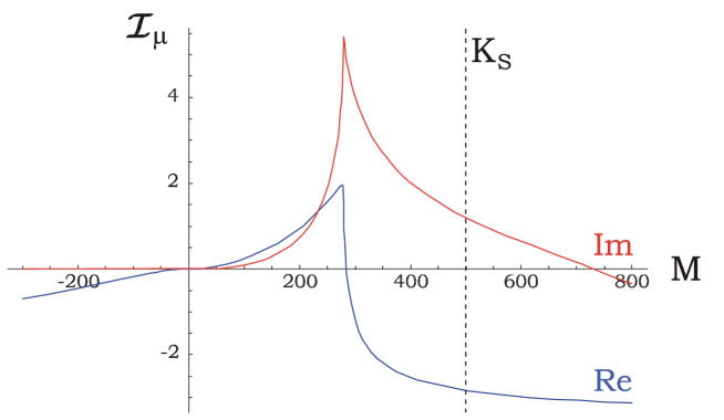
Figure 3: Behavior of $\mathcal{I}(m_{\mu}^{2}/M^{2},m_{\pi}^{2}/M^{2})$ as a function of $M$ (in MeV).

         

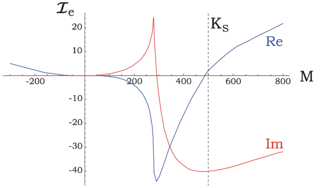
Figure 4: Behavior of $\mathcal{I}(m_{e}^{2}/M^{2},m_{\pi}^{2}/M^{2})$ as a function of $M$ (in MeV).

These analytic properties become manifest performing the integration over the $u$ variable in Eq. (30). This leads to

$$\mathrm{Re}~{}\mathcal{I}(a,b) =\displaystyle\int_{0}^{1}dx\int_{0}^{1-x}ydy\int_{0}^{1}dw\left\{\frac{x}{\alpha\gamma-\beta}\log\left|\frac{\alpha+\beta}{\alpha\left(1+\gamma\right)}\right|\right.$$ (32)

$$\qquad\qquad\left.+\frac{2x+2y-1}{\beta}\left(1-w+\left(1-\frac{\alpha}{\beta}\left(1-w\right)\right)\ln\left|\frac{\alpha+\beta}{\alpha}\right|\right)\right\}~{},$$

$$\mathrm{Im}~{}\mathcal{I}(a,b) =\displaystyle\pi\int_{0}^{1}dx\int_{0}^{1-x}ydy\int_{0}^{1}dw\frac{2x+2y-1}{2\beta}\left(1-\frac{\alpha}{\beta}\left(1-w\right)\right)\left(\frac{\left|\alpha+\beta\right|}{\alpha+\beta}-\frac{\left|\alpha\right|}{\alpha}\right)$$ (33)

$$\qquad\qquad\left.+\lim_{\varepsilon\rightarrow 0}\frac{x\left(\alpha\gamma-\beta\right)}{\left(\alpha\gamma-\beta\right)^{2}+\varepsilon^{2}}\frac{1}{2}\left(\frac{\left|\alpha+\beta\right|}{\alpha+\beta}-\frac{\left|\alpha\right|}{\alpha}+\frac{\left|1+\gamma\right|}{1+\gamma}-1\right)\right\}~{}.$$

The above representation, which holds independently of the possible signs of $\alpha$, $\beta$ and $\gamma$, takes into account all the discontinuity prescriptions and is suitable for numerical integration. This last step is actually quite delicate because, though their combination is finite, both the $PP$ and the $PP\gamma$ cuts are infrared divergent (the electron case is especially difficult since collinear singularities are much stronger). This means that large cancellations occur between the various terms of $\mathcal{I}(a,b)$. We used a numerical integration routine based on VEGAS [22], implemented in Mathematica [23] on which we relied for preventing loss of numerical significance. The results are shown in Figs. 3–4 for $P=\pi$ (where $M<0$ should be understood as $i\left|M\right|$). The behavior for $P=K$ is entirely determined by the $\gamma\gamma$ cut and it is rather smooth (as can be guessed from Figs. 3–4 below $2m_{\pi}$).

The values at $z=1$, relevant for $K_{S}\rightarrow\pi^{+}\pi^{-}\rightarrow\gamma\gamma\rightarrow\ell^{+}\ell^{-}$, are

$$\mathcal{I}\left(r_{e}^{2},r_{\pi}^{2}\right)=2.11-40.41i\;\;\;\;\;\;$$

(34)

which are compatible with the figures quoted in Ref. [11]. To further check our results, we have taken advantage of the fact that $\mathcal{A}(J^{0}\left(s\right)\rightarrow\pi^{0}\ell^{+}\ell^{-})_{\mathrm{CPC}}$ satisfies an unsubtracted dispersion relation. In particular, the reduced amplitude $\mathcal{I}\left(M^{2}\right)\equiv\mathcal{I}(m_{\ell}^{2}/M^{2},m_{P}^{2}/M^{2})$ obeys the relation

$$\operatorname{Re}\frac{\mathcal{I}\left(M^{2}\right)}{M^{2}}=\frac{P}{\pi}\int_{0}^{\infty}\frac{ds}{s-M^{2}}\operatorname{Im}\frac{\mathcal{I}\left(s\right)}{s}~{}.$$ (35)

After having computed the imaginary part over a large range of $s$ from Eq. (33), we obtained a very good agreement between the real part values found by numerical integration of (35) or directly from (32), for both $M^{2}>0$ and $M^{2}<0$. This check is particularly significant in the region $M^{2}<0$, where the integration of (32) is stable, being singularity-free, while (35) remains very sensitive to the cancellations among $PP$ and the $PP\gamma$ cuts in $\operatorname{Im}\mathcal{I}(s)$.

4.3 Total and differential rate, and inclusion of higher-order terms

Replacing the ${\cal O}(p^{2})$ amplitude $M_{\pi^{0}PP}^{(2)}(z)$ in Eq. (29) with the following parameterization

$$M_{\pi^{0}PP}^{(2)}(z)\to G_{8}m^{2}_{K}a^{P}(z)~{},$$ (36)

where $G_{8}=9.1\times 10^{-6}~{}{\rm GeV}^{2}$, the CPC differential rate becomes

$$\frac{d\Gamma_{\mathrm{CPC}}}{dz}=\frac{G_{8}^{2}m_{K}^{5}\alpha^{4}}{512\pi^{7}}\frac{r_{\ell}^{2}}{z}\beta_{\pi}(z)\beta_{\ell}^{3}(z)\left|a^{\pi}(z)\mathcal{I}\left(\frac{r_{\ell}^{2}}{z},\frac{r_{\pi}^{2}}{z}\right)-a^{K}(z)\mathcal{I}\left(\frac{r_{\ell}^{2}}{z},\frac{1}{z}\right)\right|^{2}~{}.$$ (37)

We have evaluated this expression using several parameterizations of $a^{P}(z)$, reported in Table 2. The constant one corresponds to the first approximation of Ref. [10]. The chiral forms, deduced from the $\mathcal{O}\left(p^{2}\right)$ amplitudes for $K\rightarrow\pi^{0}\pi^{+}\pi^{-}$ and $K\rightarrow\pi^{0}K^{+}K^{-}$, are the expressions which yield to the complete ${\cal O}(p^{4})$ calculation of the CPC rate. Finally, the Dalitz expression is obtained from the experimental fit of the $K_{L}\rightarrow\pi^{0}\pi^{+}\pi^{-}$ amplitude [24, 25]:

$$\mathcal{A}\left(K_{L}\rightarrow\pi^{+}\pi^{-}\pi^{0}\right)=G_{8}m_{K}^{2}a(z)+{\cal O}\left\{[p_{K}\cdot(p_{+}-p_{-})]^{2}\right\}~{},$$

$$\qquad a(z)=0.38+0.13Y_{0}-0.0059Y_{0}^{2}~{},\qquad Y_{0}=\frac{1}{r_{\pi}^{2}}\left(z-r_{\pi}^{2}-\frac{1}{3}\right)$$ (38)

neglecting the small ${\cal O}\left\{[p_{K}\cdot(p_{+}-p_{-})]^{2}\right\}$ terms. The resulting branching ratios for the muon and electron modes are shown in Table 2. The differential rate $d\Gamma/dz$ with or without the kaon loops and with the Dalitz parametrization for $a^{\pi}$ is shown in Fig. 5. As can be seen, the impact of the charged kaon loops is quite small.

	Constant	Chiral	Dalitz
$a^{\pi}(z)$	$\;\;-0.362\;\;$	$z-r_{\pi}^{2}$	$-0.46+2.44z-0.95z^{2}$
$a^{K}(z)$	$0$	$\;\;\;z-r_{\pi}^{2}-1\;\;\;$	$-$

Table 1: Phenomenological functions $a^{P}(z)$ used in the $K_{L}\rightarrow\pi^{0}P^{+}P^{-}$ vertices.

		No $KK$			Chiral $KK$
		$\text{Constant }\pi\pi$	$\text{Chiral }\pi\pi$	$\text{Dalitz }\pi\pi$	$\text{Dalitz }\pi\pi$
$\mu^{+}\mu^{-}$	${\cal B}_{\mathrm{CPC}}$	$3.48\times 10^{-12}$	$2.26\times 10^{-12}$	$2.62\times 10^{-12}$	$2.81\times 10^{-12}$
	$R_{\gamma\gamma}$	$4.15\times 10^{-6}$	$3.80\times 10^{-6}$	$3.58\times 10^{-6}$	$3.66\times 10^{-6}$
	$R_{abs}$	$81\%$	$79\%$	$77\%$	$84\%$
$e^{+}e^{-}$	${\cal B}_{\mathrm{CPC}}$	$2.28\times 10^{-14}$	$1.48\times 10^{-14}$	$1.75\times 10^{-14}$	$1.80\times 10^{-14}$
	$R_{\gamma\gamma}$	$2.73\times 10^{-8}$	$2.47\times 10^{-8}$	$2.39\times 10^{-8}$	$2.34\times 10^{-8}$
	$R_{abs}$	$27\%$	$28\%$	$30\%$	$28\%$

Table 2: Branching ratio, ratio $R_{\gamma\gamma}$ and absorptive component, $R_{abs}=\Gamma_{\mathrm{CPC}}^{abs}/\Gamma_{\mathrm{CPC}}$, for the two $K_{L}\rightarrow\pi^{0}\ell^{+}\ell^{-}$ modes, as obtained with different phenomenological expressions of $a^{\pi,K}(z)$.

         

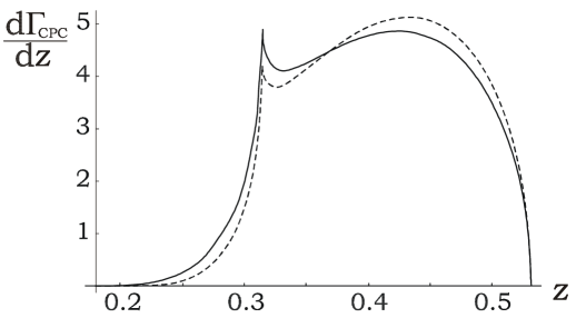
Figure 5: Differential rate for the CPC contribution, in arbitrary units, including (plain) and excluding (dashed) the $K^{+}K^{-}$ loop.

Of special interest is the ratio $R_{\gamma\gamma}$, defined in Eq. (1), with the two widths computed in terms of the same $a^{P}(z)$ vertex. Concerning the two-photon mode, this means [25]

$$\Gamma\left(K_{L}\rightarrow\pi^{0}\gamma\gamma\right)=\frac{G_{8}^{2}m_{K}^{5}\alpha^{2}}{\left(4\pi\right)^{5}}\int_{0}^{\left(1-r_{\pi}\right)^{2}}dz\;\beta_{\pi}(z)\left|a^{\pi}(z)\mathcal{I}_{\gamma\gamma}\left(z/r_{\pi}^{2}\right)-a^{K}(z)\mathcal{I}_{\gamma\gamma}(z)\right|^{2}~{},$$ (39)

with the standard loop function $\mathcal{I}_{\gamma\gamma}$ given in Ref. [19].

The phenomenological functions $a^{P}(z)$ act as a modulation of both the $\ell^{+}\ell^{-}$ and $\gamma\gamma$ spectra, and the four cases in Table 2 span a large range of behaviors (this is why we kept the constant $a^{P}$, even if this choice is clearly in conflict with chiral symmetry and the experimental $K_{L}\rightarrow\pi^{0}\gamma\gamma$ spectrum). Interestingly, the dynamics of the processes is such that $K_{L}\rightarrow\pi^{0}\gamma\gamma$ and $K_{L}\rightarrow\pi^{0}\ell^{+}\ell^{-}$ amplitudes react in a very similar way to changes in the distribution of the invariant mass of the electromagnetic system (i.e. the $\gamma\gamma$ or $\ell^{+}\ell^{-}$ pairs). As a result, despite the individual variations of the two widths, the ratio $R_{\gamma\gamma}$ remains very stable. Note that this conclusion is not induced by a complete dominance of the $2\gamma$-cut in the $K_{L}\rightarrow\pi^{0}\ell^{+}\ell^{-}$ amplitude: $\pi\pi$ and $\pi\pi\gamma$ cuts have sizable contributions, and the stability of $R_{\gamma\gamma}$ holds also for the $K_{L}\rightarrow\pi^{0}e^{+}e^{-}$ amplitude, which is dominated by the dispersive part.

As is well-known, none of the parameterizations in Table 1 for $a^{P}$ is able to reproduce both rate and spectrum of the $K_{L}\rightarrow\pi^{0}\gamma\gamma$ decay, and some additional $\mathcal{O}\left(p^{6}\right)$ genuine local terms need to be included (see e.g. Refs. [2, 26] for a recent discussion). As shown in Ref. [2], recent data point toward $\mathcal{O}\left(p^{6}\right)$ counterterms whose bulk values can be interpreted in terms of vector-meson resonances. The overall effect of these extra contributions is an enhancement of the $K_{L}\rightarrow\pi^{0}\gamma\gamma$ rate, with a spectrum which remains very similar to what we have called the Dalitz structure. Unfortunately, this information cannot be directly translated into a complete $\mathcal{O}\left(p^{6}\right)$ analysis of the $K_{L}\rightarrow\pi^{0}\ell^{+}\ell^{-}$ amplitude. However, given the stability of $R_{\gamma\gamma}$ in Table 2, we expect that $R_{\gamma\gamma}$ will not change substantially also with the inclusion of these extra $\mathcal{O}\left(p^{6}\right)$ terms. This expectation is further reinforced by the observation that the $K_{L}\rightarrow\pi^{0}\gamma\gamma$ spectrum does not show significant evidences of two-photon states with $J\not=0$ [2], and by the large size of $R_{\rm abs}$ in Table 2. Since we cannot fully determine the structure of the $K_{L}\rightarrow\pi^{0}\ell^{+}\ell^{-}$ amplitude at $\mathcal{O}\left(p^{6}\right)$, we shall attribute to our final estimate of $R_{\gamma\gamma}$ a conservative $30\%$ error, dictated by naïve chiral power counting. For the interesting muon mode, this means

$$R_{\gamma\gamma}(\ell=\mu)=(3.7\pm 1.7)\times 10^{-6}~{},$$ (40)

where the central value has been obtained from the last column in Table 2 (Dalitz expression for the pion loops and inclusion of the kaon loops).

In order to obtain the predictions of the CPC $K_{L}\rightarrow\pi^{0}\ell^{+}\ell^{-}$ widths, the estimates of $R_{\gamma\gamma}$ need to be combined with the experimental results on ${\cal B}\left(K_{L}\rightarrow\pi^{0}\gamma\gamma\right)$. The two most recent determinations

$${\cal B}\left(K_{L}\rightarrow\pi^{0}\gamma\gamma\right)^{\exp}=\left\{\begin{array}[c]{ll}\left(1.36\pm 0.03_{\rm stat}\pm 0.03_{\rm syst}\pm 0.03_{\rm norm}\right)\times 10^{-6}&\text{\cite[cite]{[\@@bibref{}{NA48_KLpgg}{}{}]}}\\ \left(1.68\pm 0.07_{\rm stat}\pm 0.08_{\rm syst}\right)\times 10^{-6}&\text{\cite[cite]{[\@@bibref{}{KTeV_KLpgg}{}{}]}}\end{array}\right.$$ (41)

leads to the average ${\cal B}\left(K_{L}\rightarrow\pi^{0}\gamma\gamma\right)^{\exp}=(1.42\pm 0.13)\times 10^{-6}$. Using this averaged result, we finally obtain

$$\begin{array}[c]{c}{\cal B}\left(K_{L}\rightarrow\pi^{0}e^{+}e^{-}\right)_{\rm CPC}^{0^{++}}=\left(3.4\pm 1.0\right)\times 10^{-14}~{},\\ {\cal B}\left(K_{L}\rightarrow\pi^{0}\mu^{+}\mu^{-}\right)_{\rm CPC}^{0^{++}}=\left(5.2\pm 1.6\right)\times 10^{-12}~{}.\end{array}$$ (42)

Given the strong helicity suppression, the result in Eq. (42) is not the dominant CPC contribution for the electron mode. As shown in Ref. [2], the constraints on the $K_{L}\rightarrow\pi^{0}\gamma\gamma$ diphoton spectrum (at low invariant mass) leave room for a $2^{++}$ CPC branching ratio, in the electron channel, around or below the $10^{-12}$ level. Because of the phase-space and angular-momentum suppression, this translates into a $10^{-14}$ contribution from $2^{++}$ in the muon mode, which can thus be safely neglected.

5 Phenomenological analysis

The total branching ratios for the two modes can be written as

$${\cal B}(K_{L}\rightarrow\pi^{0}\ell^{+}\ell^{-})=\left(C_{\rm mix}^{\ell}\pm C_{\rm int}^{\ell}\left(\frac{\displaystyle\mathrm{\operatorname{Im}}\lambda_{t}}{\displaystyle 10^{-4}}\right)+C_{\rm dir}^{\ell}\left(\frac{\displaystyle\mathrm{\operatorname{Im}}\lambda_{t}}{\displaystyle 10^{-4}}\right)^{2}+C_{\rm CPC}^{\ell}\right)\times 10^{-12},$$ (43)

with the following sets of coefficients (obtained by combining the results of the previous two sections and the analysis of Ref. [2] for $K_{L}\rightarrow\pi^{0}e^{+}e^{-}$):

$$\begin{array}[c]{lcllcl}C_{\rm mix}^{e}&=&(15.7\pm 0.3)|a_{S}|^{2}~{},&C_{\rm mix}^{\mu}&=&(3.7\pm 0.1)|a_{S}|^{2}~{},\\ C_{\rm int}^{e}&=&(6.2\pm 0.3)|a_{S}|~{},&C_{\rm int}^{\mu}&=&(1.6\pm 0.1)|a_{S}|~{},\\ C_{\rm dir}^{e}&=&2.4\pm 0.2~{},&C_{\rm dir}^{\mu}&=&1.0\pm 0.1~{},\\ C_{\rm CPC}^{e}&\approx&0~{},&C_{\rm CPC}^{\mu}&=&5.2\pm 1.6~{},\end{array}$$ (44)

where $|a_{S}|=1.2\pm 0.2$ and $\left(\operatorname{Im}\lambda_{t}/10^{-4}\right)_{\rm SM}=1.36\pm 0.12$. The Standard Model predictions are then

$$\begin{array}[]{ll}{\cal B}(K_{L}\rightarrow\pi^{0}e^{+}e^{-})=\left(3.7_{-0.9}^{+1.1}\right)\times 10^{-11}&\big{[}\left(1.7_{-0.6}^{+0.7})\times 10^{-11}\right)\big{]}~{},\\ {\cal B}(K_{L}\rightarrow\pi^{0}\mu^{+}\mu^{-})=\left(1.5\pm 0.3\right)\times 10^{-11}{~{}}^{~{}}&\big{[}~{}(1.0\pm 0.2)\times 10^{-11})~{}\big{]}~{},\end{array}$$ (45)

for positive [negative] interference. As already mentioned, several theoretical arguments point towards the constructive interference scenario [2, 18]. We report the destructive solution only for completeness, since we cannot prove yet in a model-independent way that this solution is ruled out.

         

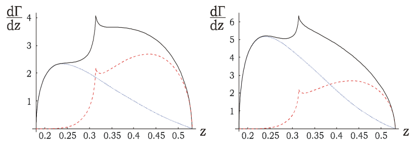
Figure 6: Differential rate for $K_{L}\rightarrow\pi^{0}\mu^{+}\mu^{-}$, in arbitrary units, for destructive (left) and constructive (right) interference. In each plot the three curves correspond to CPC (dashed), CPV (dotted) and total contribution (full).

The total differential rate and its CPC and CPV components are shown in Fig. 6 for the muon mode (the electron case is less interesting, being completely dominated by the CPV part). Although the differential CPC component is not predicted as accurately as the total one (by means of $R_{\gamma\gamma}$), it clearly emerges that the low $\mu^{+}\mu^{-}$ invariant mass region is dominated by the CPV component. This conclusion can be considered as a model-independent statement, at least at a qualitative level: it follows from the naïve distribution of $|\mu^{+}\mu^{-}\rangle$ final states with $J^{\rm CP}=1^{\pm\pm}$ (CPV) or $0^{++}$ (CPC), and it is reinforced by the experimental evidence of the $K_{L}\rightarrow\pi^{0}\gamma\gamma$ diphoton spectrum [5, 6]. For this reason, in future high-statistics experiments a cut of the high-$z$ region could be used as a powerful tool to reduce and control the CPC contamination of the signal. At a quantitative level, employing the Dalitz shape of the spectrum, we find that cutting the events with $m_{\mu\mu}>2m_{\pi}$ let us suppress about $90\%$ of the CPC contribution, while the interesting CPV term is reduced only by $40\%$ (i.e. the CPC contamination of the total rate drops to less than $10\%$).

The different shape of CPC and CPV spectra implies a suppression of their interference in the CPV distributions, such as the forward-backward (FB) asymmetry. In particular, we find that the normalized FB asymmetry integrated over the full spectrum do not exceed the ${\cal O}(10\%)$ level. Thus we do not consider this observable particularly promising for near-future (low-statistics) experiments. On the other hand, it is clear that in a long term (high-statistics) perspective this observable, as well as the other asymmetries discussed in Ref. [27], would provide a useful tool to reduce the theoretical error on the long-distance components of the $K_{L}\rightarrow\pi^{0}\mu^{+}\mu^{-}$ amplitude.

The present experimental limits on the branching ratios of the two modes can be translated into bounds on $\operatorname{Im}\lambda_{t}$, although we are clearly far from the level necessary to perform precision tests of the SM. We find

$$\begin{array}[c]{ll}{\cal B}\left(K_{L}\rightarrow\pi^{0}e^{+}e^{-}\right)<2.8\times 10^{-10}\;\text{\cite[cite]{[\@@bibref{}{KTeVelec}{}{}]}}&\rightarrow\left|\operatorname{Im}\lambda_{t}\right|<1.3\times 10^{-3}~{},\\ {\cal B}\left(K_{L}\rightarrow\pi^{0}\mu^{+}\mu^{-}\right)<3.8\times 10^{-10}\;\text{\cite[cite]{[\@@bibref{}{KTeVmuon}{}{}]}}&\rightarrow\left|\operatorname{Im}\lambda_{t}\right|<2.1\times 10^{-3}~{},\end{array}$$ (46)

where the results have been obtained without any assumption on the sign of the interference. It is worth to stress that the limit derived from the muon mode is quite close to the electron one. This happens because the phase-space suppression of the former is partially compensated by the enhancement of the helicity-suppressed terms in the (direct-CPV) axial-current contribution.

5.1 New-physics sensitivity

         

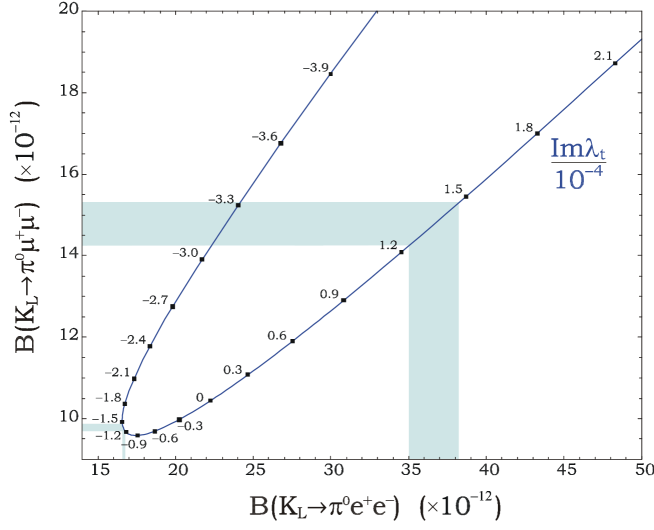
Figure 7: Central values of the two ${\cal B}(K_{L}\rightarrow\pi^{0}\ell^{+}\ell^{-})$ for various values of $\operatorname{Im}\lambda_{t}$. Negative values stand for destructive interference (see text).

As can be deduced by the comparison of Eq. (46) and Eq. (45), we still have to wait a few years before any experiment will be able to probe the two $K_{L}\rightarrow\pi^{0}\ell^{+}\ell^{-}$ modes at the SM rate. However, we recall that these two transitions are particularly sensitive to physics beyond the SM and their branching ratios could well be modified (and possibly enhanced) with respect to their SM expectations (see e.g. Refs. [30] and references therein). In such a case, the combined information on the two rates would provide a very powerful tool to identify a deviation from the SM, and also to distinguish various new-physics scenarios.

To illustrate the combined discovery potential of the two modes, it is useful to draw the curve in the ${\cal B}(K_{L}\rightarrow\pi^{0}\mu^{+}\mu^{-})$– ${\cal B}(K_{L}\rightarrow\pi^{0}e^{+}e^{-})$ plane obtained by a variation of $\operatorname{Im}\lambda_{t}$, as shown in Fig. 7. The distance between the positive and negative $\operatorname{Im}\lambda_{t}$ branches is generated by the different weights of the CPV contributions for the two modes, which in turn arise from the helicity-suppressed terms proportional to $P_{0}(z)$ and $A_{0}(z)$ in Eq. (10). In the limit where we neglect all errors but the one on $\operatorname{Im}\lambda_{t}$, as done in Fig. 7 for illustration, the SM corresponds to one small segment (or two considering also the negative interference) of this curve. Any other point along the curve corresponds to non-standard scenarios where the new-physics effect can be re-absorbed into a re-definition of $\operatorname{Im}\lambda_{t}$. Finally, the region outside the curve corresponds to non-standard scenarios with different weights of vector and axial-vector contributions.

         

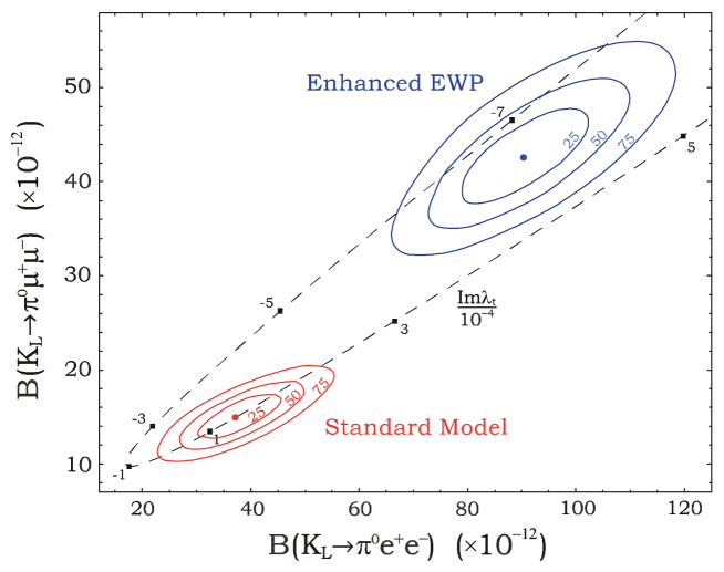
Figure 8: 25%, 50% and 75% confidence-level regions for the Standard Model (assuming positive interference) and the enhanced-electroweak-penguin model of Ref. [12], taking into account all the present uncertainties.

To discuss a concrete example, we shall consider in particular the scenario with enhanced electroweak penguins recently discussed in Ref. [12]. In this framework new physics does not modify the value of $\operatorname{Im}\lambda_{t}$, but leads to a modification of the short-distance Wilson coefficients $\bar{y}_{7V,A}\equiv y_{7V,A}/\alpha(M_{Z})$. In particular, their values are changed to $\left(\bar{y}_{7A},\bar{y}_{7V}\right)=\left(-3.2,0.9\right)$, whereas the SM case corresponds to $\left(-0.68,0.73\right)$. Given the dependence of $C_{\rm int,dir}^{\ell}$ from $\bar{y}_{7V,A}$

$$\begin{array}[c]{ll}C_{\rm int}^{e}=8.91\;\bar{y}_{7V}~{}|a_{S}|,&C_{\rm dir}^{e}=2.67\left(\bar{y}_{7V}^{2}+\bar{y}_{7A}^{2}\right)~{},\\ C_{\rm int}^{\mu}=2.12\;\bar{y}_{7V}~{}|a_{S}|,&C_{\rm dir}^{\mu}=0.63\left(\bar{y}_{7V}^{2}+\bar{y}_{7A}^{2}\right)+0.85\;\bar{y}_{7A}^{2}~{},\end{array}$$ (47)

we can easily translate this information into the corresponding predictions for the two branching ratios:

$${\cal B}(K_{L} \rightarrow\pi^{0}e^{+}e^{-})^{\rm NP}_{\rm EWP}=\left(9.0\pm 1.6\right)\times 10^{-11}~{},$$

$${\cal B}(K_{L} \rightarrow\pi^{0}\mu^{+}\mu^{-})^{\rm NP}_{\rm EWP}=\left(4.3\pm 0.7\right)\times 10^{-11}~{}.$$

Both decay widths turn out to be dominated by the direct CPV component, with a small (20%–30%) dependence from the interference sign. Since the helicity suppressed effects are proportional to the enhanced $\bar{y}_{7A}$, the relative deviation with respect to the SM prediction is larger in the muon case. As shown in Fig. 8, this scenario could clearly be distinguished from the SM case even taking into account all the present parametric uncertainties. Note that, as a consequence of the non-standard axial/vector ratio, the central point of this new-physics scenario is outside the $\operatorname{Im}\lambda_{t}$ curve.

6 Conclusions

We have presented a new comprehensive study of the rare FCNC process $K_{L}\to\pi^{0}\mu^{+}\mu^{-}$. Our main task has been a systematic analysis of the two-photon CP-conserving contribution, which represents the most delicate ingredient necessary to obtain a reliable SM prediction for the total decay rate. By means of an explicit two-loop calculation within CHPT, we have shown that this contribution can be predicted with reasonable accuracy in terms of the $K_{L}\to\pi^{0}\gamma\gamma$ width. Taking into account the experimental data on the latter [5, 6] and the recent observation of the $K_{S}\rightarrow\pi^{0}\ell^{+}\ell^{-}$ transitions [3, 4], we have been able to present the first complete SM prediction for the total branching ratio:

$${\cal B}(K_{L}\rightarrow\pi^{0}\mu^{+}\mu^{-})^{\rm SM}=\left(1.5\pm 0.3\right)\times 10^{-11}~{}.$$ (48)

This is composed by approximately equal CP-conserving, indirect-CP-violating and direct-CP-violating components (including the interference). The sizable uncertainty which affects this prediction is a parametric error which reflects the present poor experimental knowledge of the $K_{S}\to\pi^{0}\ell^{+}\ell^{-}$ rates. The irreducible theoretical error, due to the long-distance CP-conserving amplitude, is only at the $10\%$ level and, as we have shown, can be further reduced by suitable kinematical cuts.

Beside the good theoretical control of the decay rate, this channel is particularly interesting because of a different short-distance sensitivity compared to the other golden rare $K_{L}$ decays, namely $K_{L}\rightarrow\pi^{0}e^{+}e^{-}$ and $K_{L}\rightarrow\pi^{0}\nu\bar{\nu}$. As we have shown, the helicity-suppressed terms distinguish the relative weights of vector- and axial-current contributions in $K_{L}\rightarrow\pi^{0}e^{+}e^{-}$ and $K_{L}\rightarrow\pi^{0}\mu^{+}\mu^{-}$. As a result, the combination of the two decay widths could provide a very powerful tool to falsify the SM and also to distinguish among different new-physics models.

In summary, the $K_{L}\rightarrow\pi^{0}\mu^{+}\mu^{-}$ decay represents a very interesting candidate for future precision studies of CP violation and new physics in $\Delta S=1$ transitions. This mode has complementary virtues and disadvantages compared to the other rare $K$ decays, and it should be seriously considered in view of future high-statistics experiments in the kaon sector.

References

• [1] F.J. Gilman and M.B. Wise, Phys. Rev.D 21 (1980) 3150;
C. Dib, I. Dunietz and F. J. Gilman, Phys. Rev. D 39 (1989) 2639.
• [2] G. Buchalla, G. D’Ambrosio and G. Isidori, Nucl. Phys. B 672 (2003) 387 [hep-ph/0308008].
• [3] J.R. Batley et al. [NA48/1 Collaboration], Phys. Lett. B 576 (2003) 43 [hep-ex/0309075].
• [4] T.M. Fonseca Martin [NA48/1 Collaboration], talk presented at the $18^{\rm th}$ Rencontres de Physique de la Vallée d’Aoste, La Thuile, Feb 29 – Mar 6, 2004 [www.pi.infn.it/lathuile/lathuile_2004.html].
• [5] A. Lai et al. [NA48 Collaboration], Phys. Lett. B 536 (2002) 229 [hep-ex/0205010].
• [6] A. Alavi-Harati et al. [KTeV Collaboration], Phys. Rev. Lett. 83 (1999) 917 [hep-ex/9902029].
• [7] L.M. Sehgal, Phys. Rev. D 38 (1988) 808.
• [8] G. Ecker, A. Pich and E. de Rafael, Nucl. Phys. B 303 (1988) 665;
• [9] J. Flynn and L. Randall, Phys. Lett. B 216 (1989) 221.
• [10] P. Heiliger and L.M. Sehgal, Phys. Rev. D 47 (1993) 4920.
• [11] G. Ecker and A. Pich, Nucl. Phys. B 366 (1991) 189.
• [12] A. J. Buras, R. Fleischer, S. Recksiegel and F. Schwab, hep-ph/0402112.
• [13] P. Agrawal, J. N. Ng, G. Belanger and C. Q. Geng, Phys. Rev. Lett. 67 (1991) 537.
• [14] G. Ecker, A. Pich and E. de Rafael, Nucl. Phys. B 291 (1987) 692.
• [15] G. D’Ambrosio, G. Ecker, G. Isidori and J. Portolés, JHEP 08 (1998) 004 [hep-ph/9808289].
• [16] A.J. Buras, M.E. Lautenbacher, M. Misiak and M. Münz, Nucl. Phys. B 423 (1994) 349 [hep-ph/9402347]; G. Buchalla, A.J. Buras and M.E. Lautenbacher, Rev. Mod. Phys. 68 (1996) 1125 [hep-ph/9512380].
• [17] M. Battaglia et al., hep-ph/0304132.
• [18] S. Friot, D. Greynat, E. de Rafael, Rare Kaon Decays Revisited, CTP-2004/P.014; D. Greynat, talk presented at the $3^{\rm rd}$ EURIDICE Collaboration meeting, Vienna, 12 – 14 Feb 2004.
• [19] G. Ecker, A. Pich and E. de Rafael, Phys. Lett. B 189 (1987) 363.
• [20] L. Cappiello and G. D’Ambrosio, Nuovo Cim. A 99 (88) 155.
• [21] G. D’Ambrosio, G. Ecker, G. Isidori and H. Neufeld, Phys. Lett. B 380 (1996) 165 [hep-ph/9603345].
• [22] G. P. Lepage, J. Comput. Phys. 27 (1978) 192.
• [23] S. Wolfram, Mathematica – a system for doing mathematics by computer, Addison-Wesley, New York, 1988.
• [24] J. Kambor, J. Missimer and D. Wyler, Phys. Lett. B 261 (1991) 496.
• [25] A. Cohen, G. Ecker and A. Pich, Phys. Lett. B 304 (1993) 347.
• [26] F. Gabbiani and G. Valencia, Phys. Rev. D 64 (2001) 094008 [hep-ph/0105006]; ibid. D 66 (2002) 074006 [hep-ph/0207189].
• [27] M. V. Diwan, H. Ma and T. L. Trueman, Phys. Rev. D 65 (2002) 054020 [hep-ph/0112350].
• [28] A. Alavi-Harati et al. [KTeV Collaboration], hep-ex/0309072.
• [29] A. Alavi-Harati et al. [KTeV Collaboration], Phys. Rev. Lett. 84 (2000) 5279 [hep-ex/0001006].
• [30] Y. Nir and M. P. Worah, Phys. Lett. B 423 (1998) 319 [hep-ph/9711215];
A. J. Buras, A. Romanino and L. Silvestrini, Nucl. Phys. B 520 (1998) 3 [hep-ph/9712398];
G. Colangelo and G. Isidori, JHEP 09 (1998) 009 [hep-ph/9808487];
A. J. Buras et al., Nucl. Phys. B 566 (2000) 3 [hep-ph/9908371];
G. D’Ambrosio and G. Isidori, Phys. Lett. B 530 (2002) 108 [hep-ph/0112135].
• [31]