1 Introduction

The study of properties of bound states of heavy quarks plays a central role in the understanding of strong interactions and verification of different QCD inspired and nonperturbative models, because such processes give a very exciting possibility to observe interplay of ”hard” and ”soft” regimes [1]. There have been intensive experimental studies of the $J/\Psi$ and $\Upsilon$ production in $ep$ collisions at HERA [2],[3] and also a lot of theoretical investigations [4]-[8].

In this paper we consider exclusive photoproduction of $V=Q\bar{Q}_{1S}$ states from another viewpoint. There are some other interesting processes that will be investigated at present and future hadronic colliders. We need estimations of cross-sections for such processes and can use the data from HERA as a source of normalization of phenomenological models. Here we show that the extended Regge-Eikonal approach [9]-[12] gives not only a good description of the data on exclusive vector meson photoproduction but can be used also to predict rates of Exclusive Double Diffractive Events (EDDE) at LHC and Tevatron. The advantages of these events have been considered in [13],[14].

2 Calculations

In Fig. 1 we illustrate in detail the process $\gamma(q)+p(p)\to V(p_{v})+p(p^{\prime})$. Off-shell proton-gluon amplitude $T$ in Fig. 1 is treated by the method developed in Ref. [9], which is based on the extension of Regge-eikonal approach, and succesfully used for the description of the data from hadron colliders [10]-[12]. The amplitude $A$ of the process $\gamma(q)+g(\kappa_{1})\to V(p_{v})+g(\kappa_{2})$ is calculated in the nonrelativistic bound state approximation(see [4]-[6] and ref. therein):

$$A = \frac{R_{v0}}{\sqrt{16\pi M_{v}}}Sp\left[\hat{\cal{O}}(\hat{p}_{v}-M_{v})\hat{\epsilon}_{v}\right]$$ (1)

$$\hat{\cal{O}} = ee_{Q}g^{2}\frac{\delta^{ab}}{2\sqrt{3}}\left(\frac{({p_{v}}_{\alpha}-2{\kappa_{1}}_{\alpha}+\hat{\kappa}_{1}\gamma_{\alpha})\hat{\epsilon}_{\gamma}({p_{v}}_{\beta}+2{\kappa_{2}}_{\beta}-\gamma_{\beta}\hat{\kappa}_{2})}{(-p_{v}\kappa_{1}+\kappa_{1}^{2}+i0)(p_{v}\kappa_{2}+\kappa_{2}^{2}+i0)}+5\;permut.\right)\;,\;$$ (2)

where $p_{v}^{2}=M_{v}^{2}$, $e_{Q}$ is the charge of heavy quark, $R_{v0}$ is the absolute value of the vector meson radial wave function at the origin, $\epsilon_{v,\gamma}$ are photon and vector meson polarization vectors correspondingly. Permutations are taken for all gauge bosons. Notations and vector decompositions that are used in the article are

$$\kappa_{1}=\kappa+\frac{\Delta}{2}\;,\;\kappa_{2}=\kappa-\frac{\Delta}{2}\;,\;p=p^{\prime}+\frac{m_{p}^{2}}{s}q^{\prime}\;,\;q=q^{\prime}-\frac{Q^{2}}{s}p^{\prime}\;,\;$$ (3)

$$Q^{2}=-q^{2}\;,\;p^{2}=m_{p}^{2}\;,\;q^{\prime 2}=p^{\prime 2}=0\;,\;s\simeq 2p^{\prime}q^{\prime}\;,$$

$$\kappa=\frac{x_{v}}{2}(\alpha p^{\prime}+\beta q^{\prime})+\kappa_{\perp}\;,\;x_{v}=\frac{M_{v}^{2}}{s}\;,\;\kappa_{\perp}^{2}=-\vec{\kappa}^{2}\;,\;y=\frac{4\vec{\kappa}^{2}}{M_{v}^{2}}\;,\;y^{\prime}=-\frac{4\kappa^{2}}{M_{v}^{2}}\;,$$

$$\Delta=x_{v}\left(\left[1+y_{Q}+y_{\Delta}\right]p^{\prime}-y_{\Delta}q^{\prime}\right)+\Delta_{\perp}\;,\;y_{Q}=\frac{Q^{2}}{M_{v}^{2}}\;,\;t\simeq\Delta_{\perp}^{2}=-\vec{\Delta}^{2}\;,\;y_{\Delta}=\frac{\vec{\Delta}^{2}}{M_{v}^{2}}\;,$$

$$p_{v}=q+\Delta\;,\;y_{0}=\frac{m_{p}^{2}}{M_{v}^{2}}\;$$

Photon and vector meson polarization vectors in the general case ($Q\neq 0$) can be represented as follows:

$${\epsilon_{\gamma}}_{\perp}q={\epsilon_{\gamma}}_{0}q=0\;,\;{\epsilon_{\gamma}}_{\perp}^{2}=-{\epsilon_{\gamma}}_{0}^{2}=-1\;,\;{\epsilon_{\gamma}}_{0}=\frac{1}{Q}(q^{\prime}+x_{v}y_{Q}p^{\prime})\;,$$ (4)

$${\epsilon_{v}}_{\perp}p_{v}={\epsilon_{v}}_{\parallel}p_{v}=0\;,\;{\epsilon_{v}}_{\perp}=v_{\perp}+\frac{2(\vec{v}\vec{\Delta})}{s}(p^{\prime}-q^{\prime})\;,\;v_{\perp}^{2}=-\vec{v}^{2}\;,\;$$

$${\epsilon_{v}}_{\parallel}=\frac{1}{M_{v}}(q^{\prime}-x_{v}(1-y_{\Delta})p^{\prime}+\Delta_{\perp})$$

For the amplitude of the process $\gamma(q)+p(p)\to V(p_{v})+p(p^{\prime})$ we have:

$$M=\int\frac{d^{4}\kappa}{(2\pi)^{4}}\frac{1}{(\kappa_{1}^{2}+i0)(\kappa_{2}^{2}+i0)}A^{\alpha\beta,\;ab}T_{\alpha\beta,\;ab}$$ (5)

$$T_{\alpha\beta,\;ab}=\delta_{ab}\left(G_{\alpha\beta}-\frac{{P_{1}}_{\alpha}{P_{2}}_{\beta}}{P_{1}P_{2}}\right)T^{D}_{gp\to gp}\;,$$ (6)

$$G_{\alpha\beta}=g_{\alpha\beta}-\frac{{\kappa_{2}}_{\alpha}{\kappa_{1}}_{\beta}}{\kappa_{1}\kappa_{2}}\;,$$ (7)

$${P_{1}}=p-\frac{p\kappa_{1}}{\kappa_{1}\kappa_{2}}\kappa_{2}\;,\;{P_{2}}=p-\frac{p\kappa_{2}}{\kappa_{1}\kappa_{2}}\kappa_{1}\;,\;$$ (8)

Generally the amplitude $T^{D}_{gp\to gp}$ can be represented in the Regge-eikonal form [10],[12] with fixed parameters of trajectories from Ref. [12] (see Table. 1), in which the eikonal is dominated by three vacuum trajectories (Pomerons with different properties). It follows from the analysis below that at small $t$ the amplitude $T^{D}_{gp\to gp}$ takes the simple Regge form, which is dominated by the 3rd (”hard”) Pomeron:

$$T^{D}_{gp\to gp}\simeq c_{gp}\left(e^{-i\frac{\pi}{2}}\frac{2p\kappa}{s_{0}-\kappa^{2}}\right)^{\alpha_{P_{3}}(t)}e^{b^{(3)}_{0}t}\;,b^{(3)}_{0}=\frac{r^{2}_{gP_{3}}+0.5r^{2}_{pP_{3}}}{4}\;,$$ (9)

where $s_{0}\simeq 1\;GeV$ is the scale parameter of the model that is used in the global fitting of the data on $pp(p\bar{p})$ scattering [11],[12], $r^{2}_{pP_{3}}$, $\alpha_{P_{3}}(t)=\alpha_{P_{3}}(0)+\alpha^{\prime}_{P_{3}}(0)t$ are defined in Table.1, $r^{2}_{gP_{3}}$ and $c_{gp}$ are extracted by the procedure (16)-(21). With notations (3) we have:

$$d^{4}\kappa=\pi\frac{M_{v}^{4}x_{v}}{32}d\alpha d\beta dy=-\pi\frac{M_{v}^{4}x_{v}}{64}\frac{d\alpha}{\alpha}dy^{\prime}dy$$ (10)

In the limit $Q\to 0\;,\;t\to 0$ only the amplitude $M_{\perp\perp}$ survives:

$$|M_{\perp\perp}|^{2} \simeq K_{v}^{2}I_{v}(t)^{2}c_{gp}^{2}\left(\frac{s}{s_{0}}\right)^{2\alpha_{P_{3}}(0)}e^{2b_{3}t}\;,$$ (11)

$$b_{3} = b^{(3)}_{0}+\alpha^{\prime}_{P_{3}}(0)\ln\frac{s}{s_{0}}$$ (12)

$$K_{v}^{2} = \frac{4096\alpha_{e}\alpha_{s}^{2}e_{Q}^{2}|{R_{v}}_{0}|^{2}}{3M_{v}^{3}\pi^{4}}=\frac{1024\alpha_{s}^{2}\Gamma(V\to e^{+}e^{-})K_{NLO}}{3M_{v}\pi^{4}\alpha_{e}}\;,$$ (13)

$$I_{v}(t) = \int d\alpha dy^{\prime}\int_{0}^{1}dy\frac{f(\alpha,y,y^{\prime})}{(\alpha-1-y^{\prime}+i0)(\alpha+1+y^{\prime}-i0)}\cdot$$

$$\cdot \frac{1}{(\alpha y^{\prime}-y+y^{\prime}-i0)(\alpha y^{\prime}+y-y^{\prime}-i0)}$$

$$f(\alpha,y,y^{\prime}) = \frac{1}{2\alpha^{\alpha_{P_{3}}(t)-1}}\left[\frac{\alpha^{2}yy^{\prime}}{(y-y^{\prime})^{2}}\right]\left(\frac{y-y^{\prime}}{2\left(1+\frac{y^{\prime}}{4y_{0}}\right)}\right)^{\alpha_{P_{3}}(t)}$$ (15)

Now let us extract the values of parameters from the fit to the data on elastic $J/\Psi$ photoproduction [2]. At first we write the amplitude $M_{\perp\perp}$ in the Regge-eikonal form with parameters from Table.1 and the coefficient that corresponds to the simple Vector Dominance Model (VDM):

$$M_{\perp\perp}=\sqrt{\frac{3\Gamma(V\to e^{+}e^{-})}{\alpha_{e}M_{v}}}\;4\pi s\int_{0}^{\infty}db^{2}J_{0}(b\sqrt{-t})\frac{e^{2i(\delta_{1}+\delta_{2}+\delta_{3})}-1}{2i}\;,$$ (16)

where

$$\delta_{i}=i\frac{c^{(i)}_{vp}}{s_{0}}\left(e^{-i\frac{\pi}{2}}\frac{s}{s_{0}}\right)^{\alpha_{P_{i}}(0)-1}\frac{e^{\frac{-b^{2}}{\rho_{i}^{2}}}}{4\pi\rho_{i}^{2}}\;,$$ (17)

$$\rho_{i}^{2}=4\alpha^{\prime}_{P_{i}}(0)\ln\left(e^{-i\frac{\pi}{2}}\frac{s}{s_{0}}\right)+r^{2}_{gP_{i}}+0.5r^{2}_{pP_{i}}$$

As will be seen below, in our case the VDM plus Regge-eikonal approach representation (16) is applicable.

Results of this fit for $J/\Psi$ meson are shown in Figs.2-5. As we see from figures, the main contribution to the cross-section is given by the Born term of the 3rd Pomeron. The 1st ”soft” Pomeron gives no contribution. The term corresponding to the 2nd Pomeron vanishes faster with $t$, and gives the contribution less than 1%, when $t\leq-0.2\;GeV^{2}$. Numerical estimations show that absorbtive corrections play minor role at $t\simeq t^{*}=$$=-1/2b_{3}$, where $b_{3}$ is obtained from (12). Using these facts, we keep in (16) only the Born term for the 3rd Pomeron with parameters

$$r^{2}_{gP_{3}}=2.54\pm 0.41\mbox{GeV}^{-2}\;,\;c^{(3)}_{J/\Psi p}=1.11\pm 0.07\;,\;\chi^{2}/dof=1.48\;$$ (18)

and take the integral $I_{v}$ at $t=t^{*}$. Now we can estimate the constant $c_{gp}$ in (11) from the comparison of two formulae for the amplitude $M_{\perp\perp}$:

$$c_{gp}=\frac{\sqrt{\frac{3\Gamma(V\to e^{+}e^{-})}{\alpha_{e}M_{v}}}}{K_{v}I_{v}(t^{*})}\;c^{(3)}_{vp}=\frac{3\pi^{2}}{32\alpha_{s}I_{v}(t^{*})\sqrt{K_{NLO}}}\;c^{(3)}_{vp}\;,\\$$ (19)

Taking for $J/\Psi$ mesons

$$M_{J/\Psi}=3.1\;\mbox{GeV}\;,\;\alpha_{s}(M_{J/\Psi}^{2})=0.25\;,\;$$ (20)

$$I_{J/\Psi}(t^{*})\simeq 0.83\;,\;35\;\mbox{GeV}<W=\sqrt{s}<260\;\mbox{GeV}\;,$$

$$\Gamma(J/\Psi\to e^{+}e^{-})=5.26\pm 0.37\;\mbox{keV}\;,\;K_{NLO}\simeq 2\;\mbox{(see, for example, \cite[cite]{[\@@bibref{}{QQNLO}{}{}]})}$$

we get from (19):

$$c_{gp}=3.5\pm 0.4$$ (21)

Here errors are estimated from uncertanties of quantities in (19).

The data on $\Upsilon$ production [3] gives the possibility to check the model predictions. The result of ZEUS collaboration for the ratio of total cross-sections of $J/\Psi$ and $\Upsilon$ photoproduction:

$$\frac{\sigma_{\gamma p\to\Upsilon p}}{\sigma_{\gamma p\to J/\Psi p}}=(4.8\pm 2.2(\mbox{stat.}){+0.7\atop-0.6}(\mbox{sys.}))\cdot 10^{-3}$$ (22)

If we assume that the constant $c_{gp}$ is the same for both processes, and the slope of the exponent does not change much with energy, then from the expression (11) we will get at the same value of $W$:

$$\frac{\sigma_{\gamma p\to\Upsilon p}}{\sigma_{\gamma p\to J/\Psi p}}\simeq\left[\frac{\alpha_{s}(M^{2}_{\Upsilon})I_{\Upsilon}}{\alpha_{s}(M^{2}_{J/\Psi})I_{J/\Psi}}\right]^{2}\frac{\Gamma(\Upsilon\to e^{+}e^{-})K^{\Upsilon}_{NLO}M_{J/\Psi}}{\Gamma(J/\Psi\to e^{+}e^{-})K^{J/\Psi}_{NLO}M_{\Upsilon}}=(3.1\pm 1.1)\cdot 10^{-3}\;,$$ (23)

where

$$\Gamma(\Upsilon\to e^{+}e^{-})=1.32\pm 0.04\pm 0.03\;\mbox{keV}\;,$$ (24)

$$M_{\Upsilon}=9.46\;\mbox{GeV}\;,\;\alpha_{s}(M_{\Upsilon}^{2})\simeq 0.2\;,\;I_{\Upsilon}\simeq 0.21\;,$$

$$K_{NLO}\sim\frac{1}{1-\frac{16\alpha_{s}}{3\pi}}\;\mbox{(see Ref.~{}\cite[cite]{[\@@bibref{}{QQNLO}{}{}]})}\;,$$

and uncertainty of the result originates from the errors of parameters in (23). Theoretical estimation does not contradict the experimental value (22).

The second estimation can be done for the EDD dijet production at TeVatron energies. Recent CDF results [16],[17] for the upper bound of the cross-section of the process $p+p\to p+jet+jet+p$ are the following:

$$E_{T}>7\;\mbox{GeV}\;,\;\sigma<3.7\;\mbox{nb}\;,$$ (25)

$$E_{T}>10\;\mbox{GeV}\;,\;\sigma<0.97\pm 0.065\;(\mbox{stat.})\pm 0.272(\mbox{sys.})\;\mbox{nb}\;,$$

$$E_{T}>25\;\mbox{GeV}\;,\;\sigma<34\pm 5\;(\mbox{stat.})\pm 10(\mbox{sys.})\;\mbox{pb}\;.$$

After theoretical calculations by the method developed in Refs. [13],[18] we extract upper bounds for the parameter $c_{gp}$ from (25):

$$E_{T}>7\;\mbox{GeV}\;,\;c_{gp}<3.3\;,$$ (26)

$$E_{T}>10\;\mbox{GeV}\;,\;c_{gp}<3.4\;,$$

$$E_{T}>25\;\mbox{GeV}\;,\;c_{gp}<4.2\;.$$

Values of $c_{gp}$ are close to our estimation (21).

Conclusions

We can conclude that the generalized Regge-eikonal approach with 3 different Pomerons describes well the data on $J/\Psi$ production. The main contribution to the cross-section comes from the term corresponding to the 3rd, so called, ”hard” Pomeron. This makes possible to extract the corresponding parameter of the model.

The upper bound for the same parameter is found to be close to our result, when calculated from experimental estimations on EDD di-jet production made by CDF. It indicates once more the applicability of the Regge-eikonal approach and gives us the tool for further predictions.

Aknowledgements

This work is supported by the Russian Foundation for Basic Research, grant no. 04-02-17299 and partially by grant CNRS-PICS-2910.

Table 1.: Parameters $\alpha_{P_{i}}(0)$, $\alpha^{\prime}_{P_{i}}(0)$, $r^{2}_{pP_{i}}$ are obtained from the fit to the data on $p(\bar{p})+p\to p(\bar{p})+p$ [12] and remain fixed during the $J/\Psi$ data fitting.

Pomeroni	1	2	3
$\alpha_{P_{i}}(0)-1$	$0.0578\pm 0.0020$	$0.1669\pm 0.0012$	$0.2032\pm 0.0041$
$\alpha^{\prime}_{P_{i}}(0)$ (GeV-2)	$0.5596\pm 0.0078$	$0.2733\pm 0.0056$	$0.0937\pm 0.0029$
$r^{2}_{pP_{i}}$ (GeV-2)	$6.3096\pm 0.2522$	$3.1097\pm 0.1817$	$2.4771\pm 0.0964$

Figure captions

• 1: Diagram for the process $\gamma+p\to V+p$.

• 2: Diagrams for the process $\gamma+g^{*}\to V+g^{*}$.

• 3-5: Differential cross-sections of the process $\gamma+p\to V+p$ at different values of W. Solid line is the Born term for the 3rd Pomeron and dashed curve is the unitarized result.

• 6: Total cross-section of the process $\gamma+p\to V+p$. Solid line is the Born term for the 3rd Pomeron and dashed curve is the unitarized result.

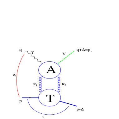
Figure 1:

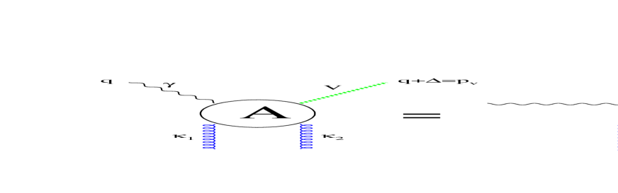
Figure 2:

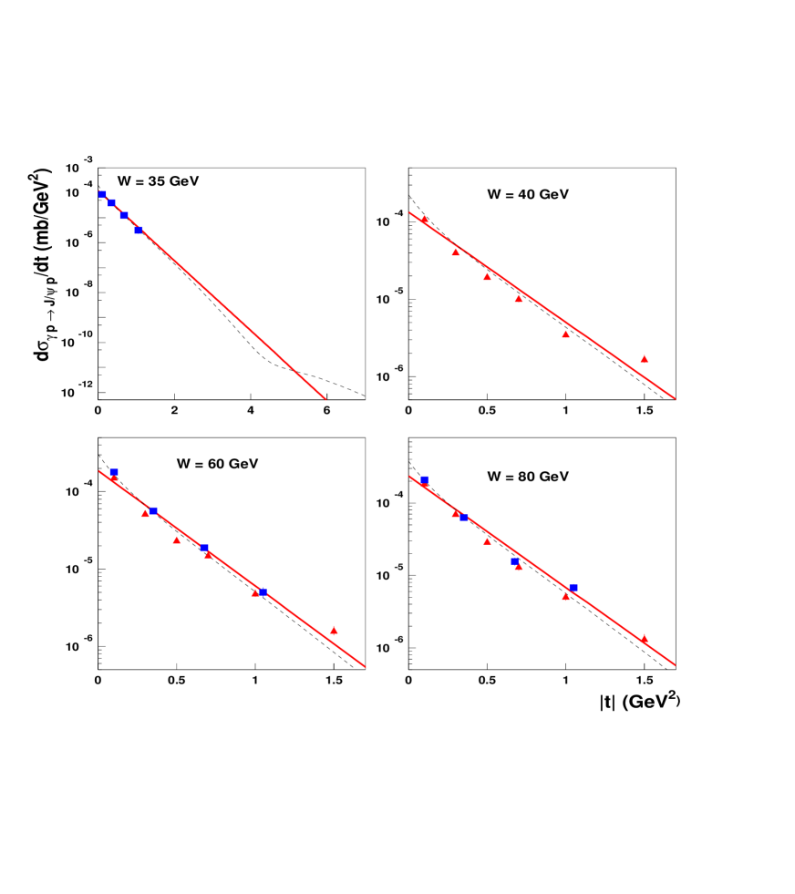
Figure 3:

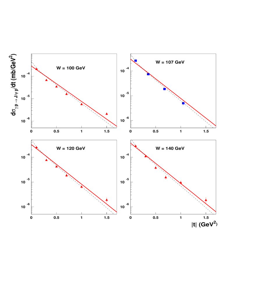
Figure 4:

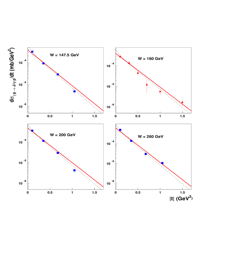
Figure 5:

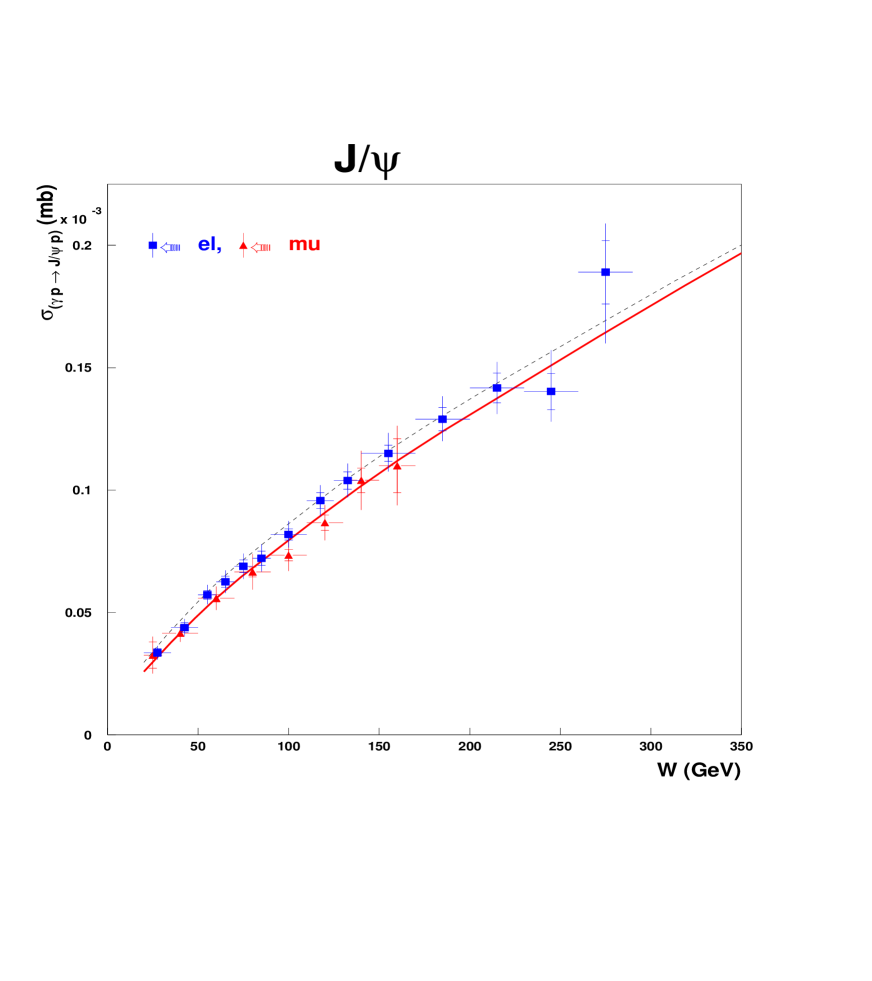
Figure 6: