What is the temperature in heavy ion collisions?

Abstract

We consider the Tsallis distribution as a source of the apparent slope of one-particle spectra in heavy-ion collisions and investigate the equation of state of this special kind of quark matter in the framework of non-extensive thermodynamics. We relate the energy per particle to the power-law tail of spectra at a given temperature.

1 Introduction

1.1 Why temperature

There is a longstanding discussion in heavy-ion physics whether the concept of temperature and the assumption of thermal equilibrium can be applied for the description of the fireball formed before hadronisation in high-energy reactions. We address here this question from the viewpoint of very rough bulk properties relating the inverse slope of one-particle transverse momentum spectra and the energy per particle. Hadron mixture fits, the so called ”thermal model” [1] assumes a constant temperature all over the fireball and obtains the energy per particle using integrals with thermal distributions: basically the Gibbs distribution, which leads to Fermi and Bose distributions in the grandcanonical treatment. Although it has been shown that due to the finiteness of the available phase space volume a canonical suppression may occur [2], the existence of temperature was not questioned in this framework.

Study of the one-particle spectra gives a reason to believe in the temperature as a universal parameter of the Gibbs distribution, $\exp(-E/T)$. From AGS through SPS to RHIC experiments the transverse momentum spectra of several particles, first of all pions, kaons and protons, show an exponential fall. This occurs in its purest form in the $p_{t}=1-4$ GeV range. At lower momenta deviations can be seen, traditionally attributed to the presence of a global transverse flow. We do not intend to discuss this part of the spectra here. At higher momenta in the RHIC experiment, however, deviations occur too. Instead of the exponential curves a power-law tail fits the experimental hadron data in the $p_{t}=4-12$ GeV range.

1.2 Why no temperature

The power law tail in the pion spectrum contradicts to the assumption of Gibbs distribution. Although one may consider the possibility that only a minor part of the particles comes from a non-equilibrated source, theoretically this doubt may be extended for the whole process. Dynamical calculations indicate that the time may not be enough to thermalize the whole spectrum before the break up [3].

In this paper we would like to test a model of hadronic and quark matter, which considers a non-exponential one-particle distribution. Such distributions with power-law tail belong to a class of anomalous distributions, not satisfying the central limit theorem of statistics. In particular the canonical Tsallis distribution, $(1+E/b)^{-c}$, which has been derived by an attempt to generalize the traditional thermodynamics [4], extrapolates between the expontial curve for $E\ll b$ and the power-law tail for $E\gg b$. The apparent temperature of the spectra is given by $T=b/c$. The Tsallis index is related to the power as $q=1-1/c$ or $q=1+1/c$ depending on the treatment of energy and particle number.

1.3 Long tailed distributions

Before reviewing the main formulae of the non-extensive thermodynamics and applying it for a massless quark-gluon plasma we remind to the central limit theorem and show a possible exemption from it. This exemption, the Lorentz distribution, has a Fourier transform corresponding to exponential transverse mass spectra after regularization.

Considering $n$ independent random variables their properly scaled sum is distributed more and more Gaussian; in the $n\rightarrow\infty$ limit exactly Gaussian. The only requirement beyond independency is that the fiducial variables must have a short range distribution.

In cases of unusual distributions, the central moments may diverge, or just not vanish for large foldness $n$. This is the case for the Lorentz-distribution, $w(x)=(T/\pi)/(1+T^{2}x^{2})$. Its Fourier transform is given by, $\tilde{w}(k)=\exp(-|k|/T)$, whose logarithm cannot be differentiated at $k=0$. The distribution $P_{n}(x)$ of $x=a_{n}\sum_{i=1}^{n}x_{i}$ has the Fourier transform $\tilde{P}_{n}(k)$ and

$$\log\tilde{P}_{n}(k)=-n|k|a_{n}/T.$$ (1)

The scaling $a_{n}=1/n$ leads in this case to a result independent of $n$ and hence to a limiting distribution, which happens to be the same Lorentzian.

Furthermore a physically supported regularization with a finite mass $m$ renders the central moments finite.

$$\tilde{w}(k)=\exp\left(\frac{m-\sqrt{k^{2}+m^{2}}}{T}\right)$$ (2)

leads to a distribution of the arithmetic sum $x=(1/n)\sum_{i=1}^{n}x_{i}$, (phyiscally interpretable as a center of mass or energy), with a Fourier transform,

$$\tilde{P}_{n}(k)=\tilde{w}^{n}(k/n)=\exp\left(\frac{nm-\sqrt{k^{2}+(nm)^{2}}}{T}\right).$$ (3)

This may be the one-particle spectra of hadrons recombined from $n$ partons each with an almost vanishing mass $m\rightarrow 0$, but with a finite total mass $M=nm$. A simple, but powerful picture of hadron formation from several partons, which leads to the experimentally observed $\exp(M-M_{t})$ transverse mass scaling spectra.

This cannot be, however, the whole story. Not only because of the power-law tail of distributions, but also on theoretical grounds. Pure recombination, as considered above, would need re-heating and expansion for not decreasing the entropy during the spontaneous hadronization. Although no detailed microdynamical description is yet known for this process, there are doubts, whether enough expansion may take place for this entropy requirement. Therefore it is of interest to circumline possible mechanisms which would change the precursor quark matter distribution into another one of the hadrons, closer to equilibrium and hence possesing higher entropy.

Such a case has been suggested in [5]. The Tsallis distribution,

$$w_{1}(E)=\left(1+E/b\right)^{-c}=w_{TS}(E,T,1-1/c),$$ (4)

after $n$-fold recombination becomes another Tsallis distrinution,

$$w_{n}(E)=\left(1+E/nb\right)^{-nc}=w_{TS}(E,T,1-1/nc),$$ (5)

much closer to the Gibbs-limit $w_{\infty}(E)=w_{TS}(E,T,1)$. It seems to be promising therefore to investigate the non-extensive thermodynamics of quark matter.

2 Tsallis distribution and energy per particle

In this paper we concentrate on the question that how large the energy per particle $E/N$ (simply related to the entropy per particle at vanishing chemical potential) can become in a quark matter with Tsallis distribution. Assuming a large enough volume for the fireball and homogenecity, we take $E/N=e/n$, the corresponding ration of densities. We shall compare this for the traditional relativistic Boltzmann gas with massless particles, for the original bag-model description of the quark-gluon plasma (QGP), and for a Tsallis-QGP with power-law tail distributed quasi-particles. We shall point out, that only the last version is able to reproduce the high value of $E/N\approx 6T$ fitted to RHIC experiments by the massive hadronic thermal model. This makes the Tsallis-QGP to an interesting candidate for the pre-hadron quark matter.

2.1 Non-extensive thermodynamics

In the following we breifly review basic formulae in the non-extensive thermodynamics. Tsallis has suggested an altered definition of entropy, which includes the Boltzmannian case as a limit. Typically it leads to a power-law tailed energy distribution instead of the exponential Gibbs-distribution, known from equilibrium statistical physics. This seems to fit for relativistic heavy ion collisions, where the observed transverse momentum spectra of hadrons definitely show a power law tail.

The Tsallis entropy contains a parameter $q$, the familiar thermodynamics is recovered in the limit $q=1$. It is given by

$$S_{q}=\frac{1}{1-q}\sum_{i}(w_{i}^{q}-w_{i})$$ (6)

with $w_{i}$ being the probability of the occurrence of the state $i$ in the statistical sample of physical states. The parameter $q$ can be related to a power characteristic to the high-energy part of these probabilities by $q=1+1/c$. The entropy can be expressed with the help of $c$ as follows

$$S_{q}=-\sum_{i}w_{i}c(w_{i}^{1/c}-1)$$ (7)

The canonical probability is obtained by maximizing the entropy (7) with a constraint on the energy and, if applies, on some charge conservation:

$$S_{q}-\beta(E-\mu N)={\rm max.}$$ (8)

Instead the sum of the energies of the individual states, $E^{\prime}=\sum_{i}w_{i}E_{i}$, and corresponding charges $N^{\prime}=\sum_{i}w_{i}Q_{i}$ in acertain version of Tsallis thermodynamics one considers the q-weighted average quantities as thermodynamical variables:

$$E=\frac{\sum_{i}w_{i}^{q}E_{i}}{\sum_{i}w_{i}^{q}},\qquad\qquad N=\frac{\sum_{i}w_{i}^{q}Q_{i}}{\sum_{i}w_{i}^{q}}.$$ (9)

One assumes that these $E$ and $N$ are additive for subsystem and reservoir parameterizing this way non-linearities (correlations) in energy and particle number. (Tsallis brings only one argument in favor of this choice against the naive one: the latter ”turns out to be inadequate for various reasons, including related to Lévy-like superdiffusion, for which a diverging second moment exists”. No reference found to this, yet.)

The optimal canonical distribution can so be obtained as

$$w_{i}=\frac{1}{Z}\exp_{c}(-x_{i}),$$ (10)

with $x_{i}=(E_{i}-\mu Q_{i})/T$. Here we introduced the parameter $T$, which we refer to as ”temperature” in the following discussion. This is, however, not equal to the inverse of the Lagrange multiplier $\beta$ [6].

The basic thermodynamical relation can be expressed, as follows:

$$-\Omega=pV=T\ln_{c}Z=TS-(E-\mu N)(1-S/c)$$ (11)

with $\ln_{c}(x)=c(1-x^{-1/c})$. This relation defines the pressure, and nicely resembles the thermodynamics in the usual form with corrections in the order of $1/c$.

The pressure is a function of $T$ and $\mu$ only in the homogeneous limit. The derivatives of the grandcanonical thermodynamical potential are

$$\frac{\partial}{\partial V}pV=p,\qquad\qquad\frac{\partial}{\partial T}pV=S,\qquad\qquad\frac{\partial}{\partial\mu}pV=N(1-S/c),$$ (12)

This helps to re-express the energy and the particle number in terms of the pressure and its derivatives:

$$N=V\frac{\frac{\partial p}{\partial\mu}}{1-\frac{V}{c}\frac{\partial p}{\partial T}},\qquad\qquad E=V\frac{\mu\frac{\partial p}{\partial\mu}+T\frac{\partial p}{\partial T}-p}{1-\frac{V}{c}\frac{\partial p}{\partial T}}.$$ (13)

It is interesting to note, that the energy per particle $E/N$ does not contain the ${\cal O}(1/c)$ correction factor directly, it resembles the usual expression

$$\frac{E}{N}=\frac{\mu\frac{\partial p}{\partial\mu}+T\frac{\partial p}{\partial T}-p}{\frac{\partial p}{\partial\mu}}.$$ (14)

We note here, that using the $E^{\prime}=\sum w_{i}E_{i}$ average energy for the canonical constraint (and similarily $N^{\prime}=\sum w_{i}Q_{i}$) leads right away to the same distribution,

$$w_{i}=\frac{1}{Z}\left(1+x_{i}/c\right)^{-c},$$ (15)

but now $q=1-1/c$ (the relation to the Tsallis index changes). Also the thermodynamics, defining $pV$ by $T\ln_{c}Z$ contains finite ${\cal O}(1/c)$ modifications:

$$TS=pV(1+S/c)+E-\mu N.$$ (16)

Now also the derivatives of the grandcanonical potential receive corresponding corrections, but the expressions for $E$ and $N$ are formally the same, as in the other case. The relation of the entropy to the pressure, however, changes,

$$S=V\frac{\frac{\partial p}{\partial T}}{1-\frac{V}{c}\frac{\partial p}{\partial T}},$$ (17)

as well as the definition of pressure now belongs to a $q$ index reflected to $1$.

Summarizing, irrespective to which Tsallis-case we choose, we define the pressure and the grandcanonical potential correspondingly, so that in both cases

$$pV=Tc(1-Z^{-1/c}).$$ (18)

The canonical distribution shows a power-law tail:

$$w_{i}=\frac{1}{Z}\frac{1}{\left(1+x_{i}/c\right)^{c}}.$$ (19)

The partition sum $Z$ is obtained by requiring $\sum_{i}w_{i}=1$.

2.2 Tsallis ideal gas, bosons, fermions

In the homogeneous case, very often encountered in simple physics models, the partition function is considered as a product of contributions from each particle state with a given momentum $\vec{k}$. The familiar logarithm of such a partition function is then additive in the phase space.

In the case of the non-equilibrium Tsallis-distribution the entropy is, however, no more additive; the above mechanism is no more trivial. Assuming that the energy, volume and particle number are still additive, the Tsallis ideal gas the following pressure:

$$p(\mu,T)=\int\frac{d^{3}k}{(2\pi)^{3}}T\ln_{c}Z,$$ (20)

with $Z$ being the one-particle Tsallis partition sum,

$$Z=\sum_{n}\exp_{c}(-nx),\qquad\qquad x=(E_{k}-\mu)/T.$$ (21)

here $\exp_{c}(x)$ is the inverse function of $\ln_{c}(x)$. This is the basis of the distinction between Fermi-Dirac and Bose-Einstein statistics: in the former case only $n=0$ and $n=1$ contributes to the sum, while in the letter case all non-negative $n$-s from zero to infinity.

The $1/c$-uncorrected derivatives of the pressure give,

$$n_{0}=\int\frac{d^{3}k}{(2\pi)^{3}}n_{c}(\frac{E_{k}-\mu}{T}),\qquad e_{0}=\int\frac{d^{3}k}{(2\pi)^{3}}E_{k}n_{c}(\frac{E_{k}-\mu}{T})$$ (22)

with

$$n_{c}(x)=-\frac{\partial}{\partial x}\ln_{c}Z(x).$$ (23)

Let us now analyze the one-particle distribution and the partition sum. First we regard the Boltzmann limit, $\exp_{c}(-x)\ll 1$. We get

$$n_{c}(x)\approx-\frac{d}{dx}\ln_{c}(1+\exp_{c}(-x))\approx-\frac{d}{dx}\exp_{c}(-x)=\left(1+\frac{x}{c}\right)^{-c-1}.$$ (24)

It is seen, that the Tsallis temperature, $T$ and the inverse slope of the logarithmic one-particle spectra somewhat differ for finite $c$ in this scenario:

$$(c+1)T_{{\rm slope}}=cT=b.$$ (25)

The product quantity, $b$ is regarded as an energy (or transverse momentum) scale which characterizes the onset of the power-law tail of the canonical Tsallis distribution. The general shape is given by

$$n_{c}(E)=\left(1+E/b\right)^{-c-1}$$ (26)

for vanishing chemical potential $\mu=0$. In this case the particle number density and energy density integrals can be calculated analytically, resulting

$$n_{0}=\frac{1}{2\pi^{2}}\frac{2b^{3}}{c(c-1)(c-2)},\qquad\qquad e_{0}=\frac{1}{2\pi^{2}}\frac{6b^{4}}{c(c-1)(c-2)(c-3)}$$ (27)

This suffices to express a relation between the inverse slope of the one-particle energy spectrum at small energy $E\ll b$, the energy per particle and the Tsallis parameter q=1+1/c:

$$E/N=e/n=\frac{3q}{4-3q}\;T_{{\rm slope}}.$$ (28)

An estimate can be given from the RHIC experiments, pointing out an inverse slope of $175$ MeV (cleaned from transverse flow effects) and $E/N=1$ GeV. This agrees with $q=1.135$ in the Boltzmann ideal gas limit of massless partons, a much more likely candidate for the pre-hadron matter, then the usual QGP: at the same $E/N$ value the massless Bose distribution leads to $T=325$ MeV temperature and slope.

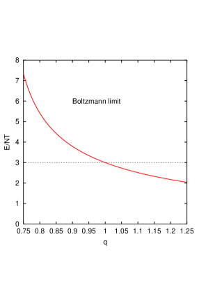
Fig. 1.: Energy per particle divided by the temperature ($E/NT$) as a function of the Tsallis index.

2.3 Finite chemical potential

We are interested in the constant $E/N$ curve on the $T-\mu$ plane for a mixture of massless bosons and fermions, which are Tsallis-distributed. Denoting $(E-qmu)/T$ generally by $x$ we deal with the following type of integral experessions:

$$n_{0}=\int dk\;k^{2}n_{c}(x)=\int_{-\mu/T}^{\infty}\!dx\;(xT+\mu)^{2}n_{c}(x).$$ (29)

Similarily for the quantity $e_{0}$, just a higher power of $(xT+\mu)$ occurs under the integral sign. The one-particle distributions $n_{c}(x)$ are for fermions or for bosons respectively.

Denoting the general integrals by $I_{n}(a)=\int_{-a}^{\infty}dx\;x^{n}n_{c}(x)$, the result consists of different power contributions. For massless fermions and antifermions together we get

$$n_{0}=T^{3}S_{2}(a)+2T^{2}\mu D_{1}(a)+T\mu^{2}S_{0}(a),$$ (30)

and

$$e_{0}=T^{4}S_{3}(a)+3T^{3}\mu D_{2}(a)++3T^{2}\mu^{2}S_{1}(a)+T\mu^{3}D_{0}(a).$$ (31)

with $S_{n}(a)=I_{n}(a)+I_{n}(-a)$ and $D_{n}(a)=I_{n}(a)-I_{n}(-a)$, $a=\mu/T$. For bosons in chemical equilibrium one takes $\mu=0$, so only the leading integrals remain, of course, in this case with Bose-Tsallis $n_{c}(x)$ functions. The energy per particle for a mixture, like quark matter, becomes

$$\frac{E}{N}=\frac{d_{B}e_{0B}(T)+d_{F}e_{0F}(T,\mu)+d_{F}e_{0F}(T,-\mu)}{d_{B}n_{0B}(T)+d_{F}n_{0F}(T,\mu)+d_{F}n_{0F}(T,-\mu)}.$$ (32)

For $c\rightarrow\infty$ one is back with the familiar Fermi-Dirac and Bose-Einstein distribution functions, and both $e_{0}$ and $n_{0}$ are finite order polynomials of $T$ and $\mu$. The ratio is a growing function of both, so a constant $E/N$ reflects in a convex curve in the $T-\mu$ plane. For large enough $c$ the Tsallis version has to behave similarily, but this question we can only decide numerically.

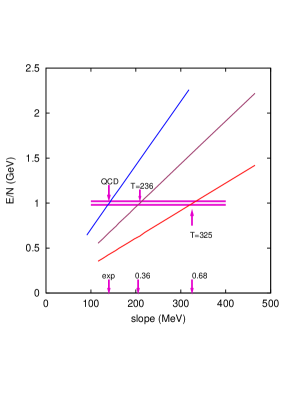
Fig. 2.: Energy per particle for massless Boson gas with Tsallis and Gibbs distributions as function of the spectral slope.

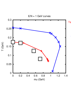
Fig. 3.: The $E/N=1$ GeV line on the temperature – chemical potential plane for the Gibbs and for the Tsallis distribution.

3 Comparison of Quark Matter Models

In conclusion we have compared three models for quark matter. The simplest, the massless Boltzmann gas, as it is long known, gives $E/N=e/n=3T$. The equation of state is given by,

$$p=\frac{1}{3}\sigma T^{4},\qquad e=\sigma T^{4},\qquad p=nT.$$ (33)

Supporting the Stefan-Boltzmann gas with a bag constant, $B$, we arrive at the traditional bag-model QGP. Now the situation is a little bit more complex. The equation of state is modified,

$$p=\frac{1}{3}\sigma T^{4}-B,\qquad e=\sigma T^{4}+B,\qquad p=nT-B.$$ (34)

This kind of matter has a stability limit at $p=0$, so the bag constant is related to a critical temperature $B=\sigma T_{cr}^{4}/3$. The energy per particle becomes at this limit $E/N=e_{cr}/n_{cr}=4T$.

Finally in a Tsallis-distributed quark matter the Stefan-Boltzmann constant $\sigma$ depends on the power $c$ (or Tsallis index $q=1-1/c$). The equation of state becomes

$$p=\frac{1}{3}\sigma(c)T^{4},\qquad e=\sigma(c)T^{4},\qquad n=\lambda(c)T^{3}.$$ (35)

The energy per particle in the Boltzmann limit is given by

$$E/N=\frac{c}{c-4}3T,$$ (36)

which is about $6T$ for $c=8$. In a bag constant supported Tsallis-QGP version one obtains, $E/N=4cT/(c-4)$ and a power of $c=12$.

References

- [1] J.Letessier, J.Rafelski, A.Tounsi, Phys.Lett. B328 (1994) 499-505; G. Torrieri, J. Rafelski, New J. Phys. 3, 12, 2003; P. Braun-Munzinger, J. Stachel, J.P. Wessels, N. Xu, Phys.Lett. B344 (1995) 43-48; P. Braun-Munzinger, J. Stachel, J. P. Wessels, N. Xu, Phys.Lett. B365 (1996) 1-6; M. Bleicher, F. M. Liu, A. Ker nen, J. Aichelin, S.A. Bass, F. Becattini, K. Redlich, K. Werner, Phys.Rev.Lett. 88 (2002) 202501; W.Broniowski, A.Baran, W.Florkowski, AIP Conf.Proc. 660 (2003) 185-195;
- [2] J. Cleymans (Cape Town, South Africa) , H. Oeschler (TU, Darmstadt), K. Redlich (Wroclaw, Poland), Phys.Lett. B485 (2000) 27-31; K. Redlich, S. Hamieh, A. Tounsi, J.Phys.G27:413-420,2001
- [3] F.M.Liu, K.Werner, J.Aichelin, M.Bleicher, H.Stoecker, J.Phys.G 30: s589-s594, 2004; M.Bleicher, H.Stoecker, J.Phys.G. 30: s111-s118, 2004
- [4] C.Tsallis, J. Stat. Phys. 52, 479 (1988), cond-mat/0312500, cond-mat/9903356, cond-mat/0012371; C.Tsallis, E.Brigatti, cond-mat/0305606; C.Tsallis, E.P.Borges, cond-mat/0301521; C.Tsallis, F.Baldovin, R.Cerbino, P.Pierobon, cond-mat/0309093; C.Anteneodo, C.Tsallis, cond-mat/0205314; L.G. Moyano, F.Baldovin, C.Tsallis, cond-mat/0305091
- [5] T.S.Biro, B.Muller, Phys.Lett. B578 (2004) 78-84
- [6] C.Tsallis, F.Baldovin, R.Cerbino, P.Pierobon, cond-mat/0309093