Abstract

We discuss the observability of CP-violating asymmetries in the process $e^{+}e^{-}\to\tilde{\chi}_{1}^{0}\tilde{\chi}_{2}^{0}\to\tilde{\chi}_{1}^{0}\tilde{\chi}_{1}^{0}\ell^{+}\ell^{-}$, with $\ell=e,\mu$. We consider two examples of supersymmetric scenarios: (i) with decays $\tilde{\chi}_{2}^{0}\to\tilde{\ell}_{R}^{\pm}\ell^{\mp}\to\tilde{\chi}_{1}^{0}\ell^{+}\ell^{-}$; (ii) with $\tilde{\chi}_{2}^{0}$ three-body decays. The asymmetries can be of order 0.1 but they are partially washed out by the large backgrounds from $W^{+}W^{-}$ and slepton pair production, being the observed asymmetries one order of magnitude smaller. However, with appropriate kinematical cuts they can be observed at an $e^{+}e^{-}$ collider with a centre of mass energy of 500 GeV and high luminosity.

1 Introduction

There are several motivations to consider further CP violation sources in addition to the CP-violating phase in the Cabibbo-Kobayashi-Maskawa matrix. From the experimental point of view, the Standard Model (SM) is unable to explain the observed baryon asymmetry of the universe. From the theoretical side, most SM extensions introduce new CP violation sources. The Minimal Supersymmetric Standard Model (MSSM) [1, 2] contains several new phases which can lead to observable effects at high energy colliders. In the neutralino sector these are the phases of the parameters $M_{1}$ and $\mu$, $\phi_{1}$ and $\phi_{\mu}$ respectively. Large phases $\phi_{1}$ and/or $\phi_{\mu}$ lead to supersymmetric contributions to electric dipole moments (EDMs) far above present limits. However, these two phases can be large without necessarily yielding unacceptably large EDMs, if there are large cancellations between the different contributions [3, 4, 5]. One of the tasks to be accomplished at a future linear collider is to explore the effects of these phases in phenomenology, in order to determine if they vanish or not.

In this paper we study the process of $\tilde{\chi}_{1}^{0}\tilde{\chi}_{2}^{0}$ production with subsequent leptonic decay of the second neutralino [6, 7, 8],

$$e^{+}e^{-}\to\tilde{\chi}_{1}^{0}\tilde{\chi}_{2}^{0}\to\tilde{\chi}_{1}^{0}\tilde{\chi}_{1}^{0}\ell^{+}\ell^{-}\,,$$ (1)

with $\ell=e,\mu$. In this process, it is possible to have a CP asymmetry in the triple product $\vec{p}_{e^{+}}\cdot(\vec{p}_{\ell^{-}}\times\vec{p}_{\ell^{+}})$ of order 0.1 for adequate choices of beam polarisations. This asymmetry is sensitive to the phases of $M_{1}$ and $\mu$ and is due to of the influence of $\tilde{\chi}_{2}^{0}$ polarisation in the $l^{+}$, $l^{-}$ angular distributions (the expressions of the polarised matrix elements for $\tilde{\chi}_{1}^{0}\tilde{\chi}_{2}^{0}$ production and $\tilde{\chi}_{2}^{0}$ decay can be found in Refs. [9, 10]). However, its experimental detection is jeopardized by the presence of huge backgrounds from the production of $W^{+}W^{-}$, selectron/smuon and, to a lesser extent, chargino pairs,

$$e^{+}e^{-} \to W^{+}W^{-}\to\ell^{+}\nu_{\ell}\,\ell^{-}\bar{\nu}_{\ell}\,,$$

$$e^{+}e^{-} \to\tilde{\ell}_{R,L}^{+}\,\tilde{\ell}_{R,L}^{-}\to\ell^{+}\tilde{\chi}_{1}^{0}\,\ell^{-}\tilde{\chi}_{1}^{0}\,,$$

$$e^{+}e^{-} \to\tilde{\chi}_{1}^{+}\tilde{\chi}_{1}^{-}\to\ell^{+}\nu_{\ell}\tilde{\chi}_{1}^{0}\,\ell^{-}\bar{\nu}_{\ell}\tilde{\chi}_{1}^{0}\,,$$ (2)

which give the same experimental signature of two oppositely charged leptons $\ell^{+}\ell^{-}$ plus missing energy and momentum. A realistic analysis taking these backgrounds into account is compulsory in order to draw a conclusion on the observability of this CP asymmetry.

We analyse two kinds of supersymmetry (SUSY) scenarios, depending on the dominant channel contributing to the decay of the second neutralino: (i) scenarios with decays $\tilde{\chi}_{2}^{0}\to\tilde{\ell}_{R}^{\pm}\ell^{\mp}\to\tilde{\chi}_{1}^{0}\ell^{+}\ell^{-}$; (ii) scenarios where $\tilde{\chi}_{2}^{0}$ has three-body decays. The case of $\tilde{\chi}_{2}^{0}\to\tilde{\ell}_{L}^{\pm}\ell^{\mp}\to\tilde{\chi}_{1}^{0}\ell^{+}\ell^{-}$ is similar to the decay to $\tilde{\ell}_{R}^{\pm}\ell^{\mp}$ but involves a heavier neutralino spectrum, for which the signal cross sections are smaller. We do not study scenarios with decays $\tilde{\chi}_{2}^{0}\to\tilde{\chi}_{1}^{0}Z\to\tilde{\chi}_{1}^{0}\ell^{+}\ell^{-}$ because the asymmetries are rather small [8], and turn out to be unobservable due to the large backgrounds. Instead of performing a scan over some region of the SUSY parameter space (for such analysis see Ref. [7], where a study complementary to this one is performed but without including backgrounds nor the effect of ISR and beamstrahlung), we concentrate on the detailed analysis of two specific examples, to illustrate each of the two situations. We consider $e^{+}e^{-}$ annihilation at a centre of mass (CM) energy of 500 GeV, as proposed for the first phase of TESLA.

This paper is organised as follows. In Section 2 we examine how CP asymmetries can be defined in $\tilde{\chi}_{1}^{0}\tilde{\chi}_{2}^{0}$ production, and fix the SUSY scenarios to be discussed. In Section 3 we analyse in detail the triple product CP asymmetry in two scenarios. The results for other scenarios are also commented. In Section 4 we summarise our results and compare with other CP violation asymmetry which is also sensitive to the phases $\phi_{1}$, $\phi_{\mu}$. In the Appendix we collect some Lagrangian terms required for our calculations.

2 CP asymmetries in $\boldsymbol{\tilde{\chi}_{1}^{0}\tilde{\chi}_{2}^{0}}$ production and decay

The process of neutralino production in Eq. (1) takes place through the diagrams depicted in Fig. 1. The Lagrangian terms and conventions used can be found in Ref. [11] and the Appendix. From inspection of the diagrams and interactions involved we can notice that only $e^{+}$ and $e^{-}$ with opposite helicities give non-vanishing contributions to the amplitude (neglecting selectron mixing), what constitutes a crucial point for the construction of our CP asymmetries. The decay of $\tilde{\chi}_{2}^{0}$ is mediated by the diagrams in Fig. 2 (production and decay diagrams are shown separately only for clarity, in our computations we calculate the complete matrix elements for the resonant process). We have omitted the diagrams with neutral scalars, which are proportional to $m_{\ell}$ and thus irrelevant for $\ell=e,\mu$.

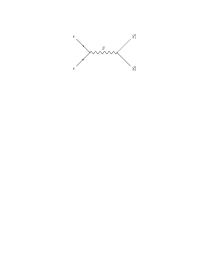
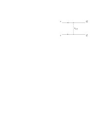
Figure 1: Feynman diagrams for $\tilde{\chi}_{1}^{0}\tilde{\chi}_{2}^{0}$ production in $e^{+}e^{-}$ annihilation.

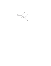
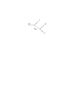
(a)		(b)		(c)

Figure 2: Feynman diagrams for the decay $\tilde{\chi}_{2}^{0}\to\tilde{\chi}_{1}^{0}\ell^{+}\ell^{-}$.

In the CM system the process of $\tilde{\chi}_{1}^{0}\tilde{\chi}_{2}^{0}$ production looks as depicted in Fig. 3, with the 3-momenta in obvious notation and $\lambda_{-}=\pm 1$, $\lambda_{+}=-\lambda_{-}$ the electron and positron helicities, respectively. The momenta of the two final state neutralinos cannot be reconstructed because of the insufficient number of kinematical constraints available for this process, thus we do not use them in our analysis. Under CP, the momenta and helicities transform as

$$\vec{p}_{e^{+}}\to-\vec{p}_{e^{-}}=\vec{p}_{e^{+}}\,,\quad\vec{p}_{e^{-}}\to-\vec{p}_{e^{+}}=\vec{p}_{e^{-}}\,,\quad\vec{p}_{\ell^{+}}\to-\vec{p}_{\ell^{-}}\,,\quad\vec{p}_{\ell^{-}}\to-\vec{p}_{\ell^{+}}\,$$

$$\lambda_{+}\to-\lambda_{-}=\lambda_{+}\,,\quad\lambda_{-}\to-\lambda_{+}=\lambda_{-}$$ (3)

(remember that in the CM frame $\vec{p}_{e^{+}}=-\vec{p}_{e^{-}}$). The initial state is CP-symmetric independently of the possible beam polarisations, owing to the fact that $\lambda_{+}=-\lambda_{-}$. Therefore, the quantities

$$Q_{1} = \vec{p}_{e^{+}}\cdot\left(\vec{p}_{\ell^{-}}\times\vec{p}_{\ell^{+}}\right)\,,$$

$$Q_{2} = \vec{p}_{e^{+}}\cdot\left(\vec{p}_{\ell^{-}}+\vec{p}_{\ell^{+}}\right)$$ (4)

are CP-odd (other higher-order CP-odd quantities may also be built using the vectors in Eqs. (3)). For $Q_{1,2}$ we define the asymmetries

$$A_{i}\equiv\frac{N(Q_{i}>0)-N(Q_{i}<0)}{N(Q_{i}>0)+N(Q_{i}<0)}\,,$$ (5)

where $N$ denotes the number of events. These asymmetries must vanish if CP is conserved, and are genuine signals of CP violation. Since $Q_{2}$ is even under naive time reversal T, in order to have a nonvanishing asymmetry $A_{2}$ the presence of CP-conserving phases in the amplitude is needed. In the process under consideration, and neglecting the small phases originated from particle widths, a nonzero $A_{2}$ arises from the interference of a dominant tree-level and a subleading loop diagram mediating the decay. Thus, $A_{2}$ is expected to be very small. On the other hand $Q_{1}$ is T-odd, and relatively large asymmetries $A_{1}$ are possible already at the tree level. We focus our analysis on the asymmetry $A_{1}$. We note that particle-antiparticle identification is necessary in order to build a triple product CP asymmetry in this process. In hadronic decays $\tilde{\chi}_{2}^{0}\to\tilde{\chi}_{1}^{0}q\bar{q}$ one could try to build an analogous asymmetry distinguishing the two quark jets by their energy. However, a triple product such as $\vec{p}_{e^{+}}\cdot\left(\vec{p}_{q_{1}}\times\vec{p}_{q_{2}}\right)$ is CP-even, and at least three untagged jets in the final state are required to construct a CP-odd triple product.

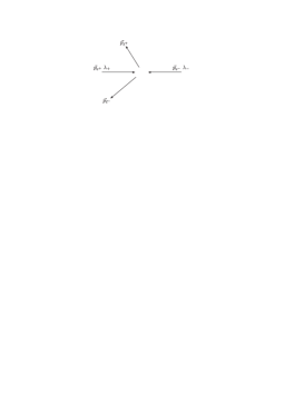
Figure 3: Schematic picture of the process $e^{+}e^{-}\to\tilde{\chi}_{1}^{0}\tilde{\chi}_{2}^{0}\to\tilde{\chi}_{1}^{0}\tilde{\chi}_{1}^{0}\ell^{+}\ell^{-}$ in the CM frame.

In the presence of a “symmetric” background the observed asymmetry $A_{1}^{\mathrm{eff}}$ is smaller than $A_{1}$ because the background does not contribute to the numerator of Eq. (5) but contributes to the denominator. If we define the ratio

$$r=\frac{S}{S+B}\,,$$ (6)

$S$ and $B$ denoting the number of signal and background events, respectively, the effective asymmetry and its statistical error are

$$A_{1}^{\mathrm{eff}}=rA_{1}\,,\quad\Delta A_{1}^{\mathrm{eff}}\simeq\sqrt{r}\Delta A_{1}\,,$$ (7)

where the statistical error of the signal alone is $\Delta A_{1}=\sqrt{(1-A_{1}^{2})/S}$. The second relation in Eq. (7) holds to a very good accuracy for the values of $A_{1}$ found in this work. Then, with the presence of a background which does not have a CP asymmetry, the statistical significance $A_{1}/\Delta A_{1}$ decreases by a factor $\sqrt{r}$.

Our first supersymmetric scenario is very similar to the scenario SPS1a in Ref. [12]. The parameters relevant for our analysis are collected in Table 1. They approximately correspond to $m_{1/2}=250$ GeV, $m_{\tilde{E}}=m_{\tilde{L}}=m_{H_{i}}=100$ GeV, $A_{E}=-100$ GeV at the unification scale, and $\tan\beta=10$. In this scenario, the diagrams dominating $\tilde{\chi}_{2}^{0}\to\tilde{\chi}_{1}^{0}\ell^{+}\ell^{-}$ are those with decay to on-shell sleptons $\tilde{\ell}_{R}^{\pm}$ in Fig. 2c, 2b. For a heavier slepton spectrum (and the same $\tilde{\chi}_{2}^{0}$ mass) two-body decays are not kinematically allowed, and $\tilde{\chi}_{2}^{0}$ has three-body decays. This corresponds to our second scenario, with $m_{\tilde{E}}=m_{\tilde{L}}=m_{H_{i}}=200$ GeV, $A_{E}=-200$ GeV. In both scenarios $\tilde{\chi}_{1}^{0}$ and $\tilde{\chi}_{2}^{0}$ are gaugino-like and $\tilde{\chi}_{1}^{0}$ is mainly a bino. We also comment on the the situation when there is more mixing in the neutralino sector, so that $\tilde{\chi}_{1}^{0}$ has a sizeable wino component.

Parameter		Scenario 1		Scenario 2
$M_{1}$		101.8 $e^{i\phi_{1}}$		102.0 $e^{i\phi_{1}}$
$M_{2}$		191.8		192.0
$\mu$		358.5 $e^{i\phi_{\mu}}$		377.5 $e^{i\phi_{\mu}}$
$\tan\beta$		10		10
$m_{\tilde{e}_{R}},m_{\tilde{\mu}_{R}}$		142.5		224.0
$m_{\tilde{e}_{L}},m_{\tilde{\mu}_{L}}$		200.7		264.5
$m_{\tilde{\chi}_{1}^{0}}$		98.7		99.1
$m_{\tilde{\chi}_{2}^{0}}$		176.4		178.1

Table 1: Low-energy parameters (at the scale $M_{Z}$) for the two SUSY scenarios discussed. The dimensionful parameters are in GeV. The neutralino masses correspond to $\phi_{1}=0$, $\phi_{\mu}=0$, and differ less than $\pm 3$ GeV for other phases.

We have checked that in both scenarios it is possible to have the electron EDM $d_{e}$ below the present experimental limit $d_{e}^{\mathrm{\,exp}}=(0.079\pm 0.074)\times 10^{-26}~{}e$ cm [13]. Using the expressions for the electron EDM in Ref. [14], we find that for each value of $\phi_{1}$ between 0 and $2\pi$ it is possible to find a narrow interval for $\phi_{\mu}$ (which can be chosen such that $|\phi_{\mu}|\leq 0.08$ in scenario 1 and $|\phi_{\mu}|\leq 0.12$ in scenario 2) in which the chargino and neutralino contributions to $d_{e}$ cancel, resulting in a value compatible with experiment. In our numerical calculations we let $\phi_{1}$ vary freely and set $\phi_{\mu}=0$, bearing in mind that their values are strongly correlated but our CP asymmetries and cross sections are insensitive to the small variation of $\phi_{\mu}$ in the ranges required for the cancellations of the EDMs ($|\phi_{\mu}|\leq 0.08$, $|\phi_{\mu}|\leq 0.12$).

3 Results

We calculate the matrix elements for the resonant processes in Eqs. (1,2) using HELAS [15], so as to include all spin correlations and finite width effects. We assume a CM energy of 500 GeV and an integrated luminosity of 345 fb^-1 per year [16]. In our calculation we take into account the effects of initial state radiation (ISR) [17] and beamstrahlung [18, 19], using for the latter the design parameters $\Upsilon=0.05$, $N=1.56$ [16]. We also include a beam energy spread of 1%. In order to simulate the calorimeter and tracking resolution, we perform a Gaussian smearing of the energies of electrons and muons using the specifications in the TESLA Technical Design Report [20]

$$\frac{\Delta E^{e}}{E^{e}}=\frac{10\%}{\sqrt{E^{e}}}\oplus 1\%\;,\quad\frac{\Delta E^{\mu}}{E^{\mu}}=0.02\%\,E^{\mu}\;,$$ (8)

where the energies are in GeV and the two terms are added in quadrature. We apply “detector” cuts on transverse momenta, $p_{T}\geq 10$ GeV, and pseudorapidities $|\eta|\leq 2.5$, the latter corresponding to polar angles $10^{\circ}\leq\theta\leq 170^{\circ}$. We also reject events in which the leptons are not isolated, requiring a “lego-plot” separation $\Delta R=\sqrt{\Delta\eta^{2}+\Delta\phi^{2}}\geq 0.4$. We do not require specific trigger conditions, and we assume that the presence of charged leptons with high transverse momentum will suffice. For the Monte Carlo integration in 6-body phase space we use RAMBO [21].

3.1 Scenarios 1 and 2

The dependence of the asymmetry $A_{1}$ on the phase $\phi_{1}$ (taking $\phi_{\mu}=0$) is shown in Fig. 4 for the two scenarios under study and three polarisation choices. In these plots we consider ISR, beamstrahlung, beam spread and detector effects, but do not include backgrounds. We observe that for $P_{e^{+}}=0.6$, $P_{e^{-}}=-0.8$ the asymmetry is slightly larger than in the unpolarised case, while it is significantly reduced for $P_{e^{+}}=-0.6$, $P_{e^{-}}=0.8$. For completeness, we show in Fig. 5 the dependence of $A_{1}$ on $\phi_{\mu}$ for $\phi_{1}=0$. For the two polarisation choices which turn out to be of interest for this process ($P_{00}$ and $P_{+-}$) the asymmetry is virtually independent of $\phi_{\mu}$. The cross sections of the signal and backgrounds are plotted in Figs. 6–8 as a function of $\phi_{1}$. $\tilde{\chi}_{1}^{0}\tilde{\chi}_{2}^{0}$ production is largest for $P_{e^{+}}=0.6$, $P_{e^{-}}=-0.8$ because the dominant contributions to the amplitude are from $\tilde{e}_{L}$ exchange diagrams in both scenarios. These polarisations enhance the $W^{+}W^{-}$ cross section, which is the largest background, but reduce $\tilde{\ell}_{R}\tilde{\ell}_{R}$ production which is the second one in importance. It is clear from Figs. 4–8 that in both scenarios this polarisation choice yields the best sensitivity for the measurement of $A_{1}$. We note here that the determination of $\phi_{1}$ from a cross section measurement does not seem possible, due not only to the small relative variation of the total (signal plus background) cross section but also to the theoretical uncertainties regarding neutralino mixing, sparticle mass spectrum, scale dependence of the cross sections, etc.

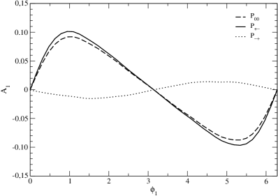
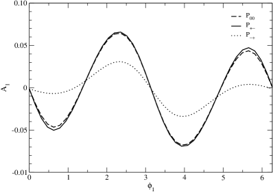
(a)	(b)

Figure 4: Dependence of the asymmetry $A_{1}$ on the phase $\phi_{1}$ in scenario 1 (a) and scenario 2 (b). Backgrounds are not included. We consider unpolarised beams ($P_{00}$), $P_{e^{+}}=0.6$, $P_{e^{-}}=-0.8$ ($P_{+-}$) and $P_{e^{+}}=-0.6$, $P_{e^{-}}=0.8$ ($P_{-+}$).

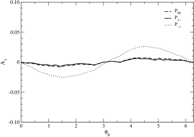
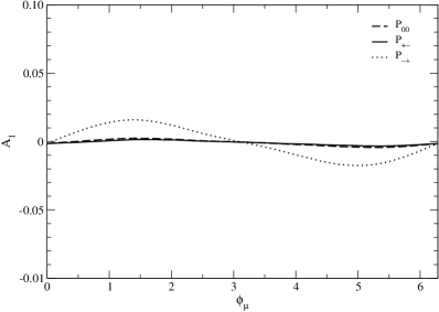
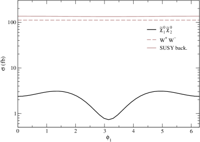
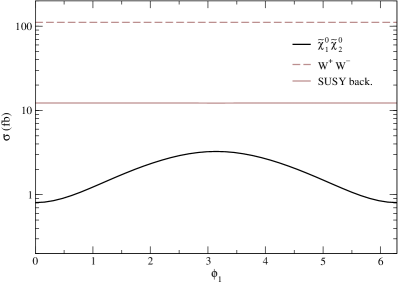
(a)	(b)

Figure 5: Dependence of the asymmetry $A_{1}$ on the phase $\phi_{\mu}$ in scenario 1 (a) and scenario 2 (b). Backgrounds are not included. We consider unpolarised beams ($P_{00}$), $P_{e^{+}}=0.6$, $P_{e^{-}}=-0.8$ ($P_{+-}$) and $P_{e^{+}}=-0.6$, $P_{e^{-}}=0.8$ ($P_{-+}$).

(a)	(b)

Figure 6: Dependence of the signal and background cross sections on the phase $\phi_{1}$ in scenario 1 (a) and scenario 2 (b), for unpolarised beams.

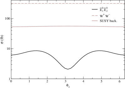
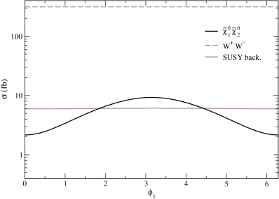
(a)	(b)

Figure 7: Dependence of the signal and background cross sections on the phase $\phi_{1}$ in scenario 1 (a) and scenario 2 (b), for $P_{e^{+}}=0.6$, $P_{e^{-}}=-0.8$.

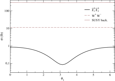
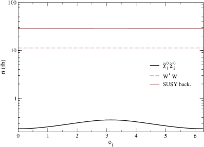
(a)	(b)

Figure 8: Dependence of the signal and background cross sections on the phase $\phi_{1}$ in scenario 1 (a) and scenario 2 (b), for $P_{e^{+}}=-0.6$, $P_{e^{-}}=0.8$.

The $W^{+}W^{-}$ background can be effectively reduced requiring that the angle $\theta$ between the two final state charged leptons is smaller than, for instance, $90^{\circ}$ (we have not attempted to optimise the signal to background ratio but rather we have chosen $\theta\leq 90^{\circ}$ in all cases for simplicity). The kinematical distribution of the signal and backgrounds with respect to $\cos\theta$ is shown in Fig. 9, with all cross sections normalised to unity. The total cross sections are: $\sigma_{W^{+}W^{-}}=318$ fb; $\sigma_{\tilde{\chi}_{1}^{0}\tilde{\chi}_{2}^{0}}=6.2~{}(2.2)$ fb, $\sigma_{\tilde{\ell}\tilde{\ell}}=52.1~{}(3.0)$ fb, $\sigma_{\tilde{\chi}_{1}^{+}\tilde{\chi}_{1}^{-}}=1.2\times 10^{-3}~{}(2.9)$ fb in scenario 1 (scenario 2). $W^{+}W^{-}$ production is strongly peaked at $\theta=180^{\circ}$, because $W^{+}W^{-}$ pairs are produced with high momentum in the CM frame and in the $W$ rest frame the charged lepton is preferrably emitted in the direction of the $W$ boson CM momentum. Slepton decays are isotropic, thus the only dependence on the angle $\theta$ of the $\tilde{\ell}\tilde{\ell}$ cross section is kinematical. It can be noticed that the decrease with $\cos\theta$ of their cross section is more pronounced in scenario 1 (in this case the sleptons are lighter and then produced with larger energy and momentum).

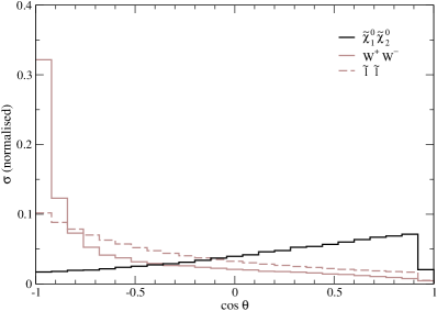
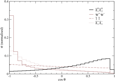
(a)	(b)

Figure 9: Dependence of the signal and background cross sections on the angle $\theta$ between $\ell^{+}$ and $\ell^{-}$ in scenario 1 (a) and scenario 2 (b). We have set $\phi_{1}=0$ and $P_{e^{+}}=0.6$, $P_{e^{-}}=-0.8$. All cross sections are normalised to unity.

One could expect that the $W^{+}W^{-}$ background had smaller values of the missing transverse momentum $p_{T}\!\!\!\!\!\!\!\!\!\not\,\,\,\,\,\,\,\,$ than SUSY processes, in which there is a pair of heavy undetected $\tilde{\chi}_{1}^{0}$ in the final state. However, as we observe in Fig. 10, the kinematical distributions are not so different, and trying to reduce the background requiring large $p_{T}\!\!\!\!\!\!\!\!\!\not\,\,\,\,\,\,\,\,$ eliminates a large fraction of the signal. The results for the observed asymmetry $A_{1}^{\mathrm{eff}}$ (including backgrounds) are presented in Fig. 11 for both scenarios, using $P_{e^{+}}=0.6$, $P_{e^{-}}=-0.8$, which give the best results, and requiring $\theta\leq 90^{\circ}$. We also show the statistical error for two years with a luminosity of 345 fb^-1 per year. Comparing with Fig. 4 we see that the asymmetry roughly decreases by a factor $r\sim 1/10$ due to the backgrounds, but it can be observed after a few years of running for wide ranges of $\phi_{1}$. We remark that detector and kinematical cuts do not generate by themselves a “fake” asymmetry $A_{1}$ (the asymmetry goes to zero when CP is conserved). Still, the cut $\theta\leq 90^{\circ}$ slightly enhances the values of $A_{1}$ when they are nonzero.

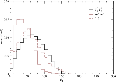
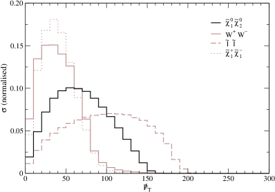
(a)	(b)

Figure 10: Kinematical distribution of the missing transverse momentum $p_{T}\!\!\!\!\!\!\!\!\!\not\,\,\,\,\,\,\,\,$ in scenario 1 (a) and scenario 2 (b). We have set $\phi_{1}=0$ and $P_{e^{+}}=0.6$, $P_{e^{-}}=-0.8$. All cross sections are normalised to unity.

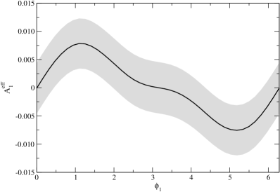
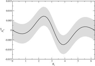
(a)	(b)

Figure 11: Dependence of the observed asymmetry $A_{1}^{\mathrm{eff}}$ (including backgrounds) on the phase $\phi_{1}$ in scenario 1 (a) and scenario 2 (b), for $P_{e^{+}}=0.6$ and $P_{e^{-}}=-0.8$. The shaded area represents the statistical error for two years of running.

We collect in Table 2 the signal and background cross sections for two examples in which the observability of the CP asymmetry is nearly maximal: $\phi_{1}=\pi/3$ in scenario 1 and $\phi_{1}=3\pi/4$ in scenario 2. The kinematical cut on $\theta$ reduces $W^{+}W^{-}$ and $\tilde{\ell}\tilde{\ell}$ production by factors of 6 and $2-3$, respectively, while keeping approximately 70% of the signal. The CP asymmetries before cuts in these scenarios are $A_{1}=0.101$, $A_{1}=0.066$, and after cuts they are $A_{1}=0.108$, $A_{1}=0.074$. The ratio $r$ after cuts is $r=0.074$, $r=0.097$, yielding effective asymmetries $A_{1}^{\mathrm{eff}}=0.0080$, $A_{1}^{\mathrm{eff}}=0.0072$. These asymmetries can be observed with statistical significances of $1.8\,\sigma$ and $1.5\,\sigma$, respectively, after two years of running.

	Scenario 1		Scenario 2
	before	after	before	after
$\tilde{\chi}_{1}^{0}\tilde{\chi}_{2}^{0}$	8.18	5.49	7.83	6.01
$W^{+}W^{-}$	318.0	54.3	318.0	54.3
$\tilde{\ell}^{+}\tilde{\ell}^{-}$	53.1	14.2	3.11	1.33
$\tilde{\chi}_{1}^{+}\tilde{\chi}_{1}^{-}$	$\sim 10^{-3}$		2.96	0.56

Table 2: Cross sections (in fb) before and after kinematical cuts of the signal and backgrounds in scenario 1 (a) and scenario 2 (b). In the first scenario we choose $\phi_{1}=\pi/3$, and in the second $\phi_{1}=3\pi/4$.

3.2 Other SUSY scenarios

In the two scenarios analysed in detail the asymmetry $A_{1}$ is difficult to observe due to the fact that the same beam polarisations $P_{e^{+}}=0.6$, $P_{e^{-}}=-0.8$ which make the signal largest also enhance the most important background, which is $W^{+}W^{-}$ production, and for $P_{e^{+}}=-0.6$, $P_{e^{-}}=0.8$ the signal is small, because $\tilde{e}_{L}$ exchange dominates the amplitudes of $e^{+}e^{-}\to\tilde{\chi}_{1}^{0}\tilde{\chi}_{2}^{0}$. One can then wonder what is the situation in SUSY scenarios where $\tilde{e}_{R}$ exchange is important, so that $\tilde{\chi}_{1}^{0}\tilde{\chi}_{2}^{0}$ production is large with the latter choice of beam polarisations. The situation does not improve however, because these polarisations increase the cross section for $\tilde{\ell}_{R}\tilde{\ell}_{R}$ production, which is the second largest background and more difficult to remove with kinematical cuts (see Figs. 9,10). We have explicitly analysed one scenario with large neutralino mixing, finding results very similar to those presented in the previous subsection. The parameters for this scenario are: $M_{1}=105.8\,e^{i\phi_{1}}$ GeV, $M_{2}=199.3$ GeV, $\mu=263.5\,e^{i\phi_{\mu}}$ GeV, $m_{\tilde{L}}=m_{\tilde{E}}=100$ GeV, $A_{E}=0$, $\tan\beta=10$. The relevant sparticle masses are $m_{\tilde{e}_{R},\tilde{\mu}_{R}}=147.5$ GeV, $m_{\tilde{e}_{L},\tilde{\mu}_{L}}=211.5$ GeV, $m_{\tilde{\chi}_{1}^{0}}\simeq 103$ GeV, $m_{\tilde{\chi}_{2}^{0}}\simeq 174$ GeV, close to the values for scenario 1. We have found that in the best case the asymmetry can be observed with $1.2\,\sigma$ after two years of running. More favourable SUSY scenarios may be found, but the general trend is that the CP asymmetry $A_{1}$ is difficult to observe, due either to the $W^{+}W^{-}$ background or the $\tilde{\ell}_{R}\tilde{\ell}_{R}$ background.

4 Summary and conclusions

The determination of the presence (or not) of complex phases in the neutralino sector is one of the tasks that must be carried out at a future linear collider. This will be done following two different approaches: with a precise analysis of CP-conserving quantities (see e.g, Refs. [22, 23, 24]) and through the investigation of CP-violating asymmetries. We have shown that in $\tilde{\chi}_{1}^{0}\tilde{\chi}_{2}^{0}$ production it is possible to have a CP asymmetry in the triple product $\vec{p}_{e^{+}}\cdot(\vec{p}_{\ell^{-}}\times\vec{p}_{\ell^{+}})$ which is very sensitive to the phase $\phi_{1}$ of the gaugino mass $M_{1}$. We have studied two SUSY scenarios, one with $\tilde{\chi}_{2}^{0}\to\tilde{\ell}_{R}^{\pm}\ell^{\mp}$ and the other with three-body decays of $\tilde{\chi}_{2}^{0}$. In both scenarios the neutralinos are light enough to be accessible at a CM energy of 500 GeV, as proposed for the first phase of TESLA and NLC. The CP asymmetries in $\tilde{\chi}_{1}^{0}\tilde{\chi}_{2}^{0}$ production are of order 0.1, and the “effective” asymmetries observed (which include the backgrounds) are roughly one order of magnitude smaller. At any rate, asymmetries of order 0.01 can be observed after a few years of running with the planned luminosity, for wide intervals of $\phi_{1}$. The results for a heavier SUSY spectrum are similar, and could be experimentally studied with higher CM energies and luminosities.

It should be emphasised that this study is complementary to the analysis of CP asymmetries in other processes. Selectron cascade decays $\tilde{e}_{L}\to e\tilde{\chi}_{2}^{0}\to e\tilde{\chi}_{1}^{0}\mu^{+}\mu^{-}$ are one example, where there may exist a CP asymmetry in the triple product $\vec{s}\cdot(\vec{p}_{\mu^{-}}\times\vec{p}_{\mu^{+}})$, with $\vec{s}$ the $\tilde{\chi}_{2}^{0}$ spin [25]. In the scenario with $\tilde{\chi}_{2}^{0}$ three-body decays discussed, it is easier to observe a CP asymmetry in the latter process. In particular, the asymmetry in $\tilde{\chi}_{1}^{0}\tilde{\chi}_{2}^{0}$ production is negligible for $\phi_{1}=\pi/2$, $\phi_{1}=3\pi/2$, whereas in selectron decays it is nearly maximal. The reverse situation occurs in the scenario with decays $\tilde{\chi}_{2}^{0}\to\tilde{\ell}_{R}^{\pm}\ell^{\mp}$: the asymmetry in selectron decays is very small, while it could be observable in $\tilde{\chi}_{1}^{0}\tilde{\chi}_{2}^{0}$ production for values of $\phi_{1}$ around $\pm 1$. The combined analysis of these and other processes, together with the constraints from EDMs, may allow the determination of the CP-violating phases in the neutralino sector.

Acknowledgements

This work has been supported by the European Community’s Human Potential Programme under contract HTRN–CT–2000–00149 Physics at Colliders and by FCT through projects POCTI/FNU/43793/2002, CFIF–Plurianual (2/91) and grant SFRH/ BPD/12603/2003.

Appendix A Notation and conventions

We list here some of the mass matrices and interactions used in this work, (see also Ref. [11]) following the conventions of Ref. [26]. We neglect flavour mixing and assume that the trilinear terms are real.

The relation between slepton mass eigenstates $\tilde{\ell}=(\tilde{\ell}_{1}~{}\tilde{\ell}_{2})^{T}$ (with $m_{\tilde{\ell}_{1}}<m_{\tilde{\ell}_{2}}$) and weak interaction eigenstates $\tilde{\ell}^{\prime}=(\tilde{\ell}_{L}~{}\tilde{\ell}_{R})^{T}$ can be written as $\tilde{\ell}=R^{\tilde{\ell}}\,\tilde{\ell}^{\prime}$, with

$$R^{\tilde{\ell}}=\left(\begin{array}[]{cc}\sin\theta_{\tilde{\ell}}&\cos\theta_{\tilde{\ell}}\\ -\cos\theta_{\tilde{\ell}}&\sin\theta_{\tilde{\ell}}\end{array}\right)\,.$$ (A.1)

In the basis where $\psi^{+}=(\tilde{W}^{+},\tilde{H}_{2}^{+})^{T}$, $\psi^{-}=(\tilde{W}^{-},\tilde{H}_{1}^{+})^{T}$, the chargino mass term is

$$\mathcal{L}_{\tilde{\chi}^{\pm}}^{\mathrm{mass}}=-(\psi^{-})^{T}M_{\tilde{\chi}^{\pm}}\,\psi^{+}+\mathrm{H.c.}\,,$$ (A.2)

being the chargino mass matrix

$$M_{\tilde{\chi}^{\pm}}=\left(\begin{tabular}[]{cc}$M_{2}$&$\sqrt{2}\,m_{W}\sin\beta$\\ $\sqrt{2}\,m_{W}\cos\beta$&$\mu$\end{tabular}\right)\,.$$ (A.3)

This matrix can be diagonalised with two unitary matrices $U$ and $V$,

$$U^{*}M_{\tilde{\chi}^{\pm}}V^{\dagger}=M_{\tilde{\chi}^{\pm}}^{\mathrm{diag}}\,.$$ (A.4)

The physical chargino fields are $\tilde{\chi}_{i}^{-}=\left(\chi_{i}^{-}~{}\overline{\chi_{i}^{+}}\right)^{T}$, with $\chi^{-}=U\psi^{-}$, $\chi^{+}=V\psi^{+}$. Their couplings to leptons are

$$\mathcal{L}_{\tilde{\nu}_{\ell}\ell\tilde{\chi}_{j}^{-}} = \tilde{\nu}_{\ell}\;\bar{\ell}\left[B_{Lj}^{\ell}P_{L}+B_{Rj}^{\ell}P_{R}\right]\tilde{\chi}_{j}^{-}+\mathrm{H.c.}\,,$$

$$\mathcal{L}_{\tilde{\ell}_{i}\nu_{\ell}\tilde{\chi}_{j}^{-}} = \tilde{\ell}_{i}^{*}\;\bar{\nu}_{\ell}\left[B_{Lij}^{\nu}P_{L}\right]\tilde{\chi}_{j}^{-}+\mathrm{H.c.}\,,$$ (A.5)

with

$$B_{Lj}^{\ell} = Y_{\ell}\,U_{j2}^{*}\,,$$

$$B_{Rj}^{\ell} = -g\,V_{j1}\,,$$

$$B_{Lij}^{\nu} = -g\,U_{j1}^{*}\,R_{i1}^{\tilde{\ell}}+Y_{\ell}\,U_{j2}^{*}\,R_{i2}^{\tilde{\ell}}\,.$$ (A.6)

For $\ell=e,\mu$ the terms with the Yukawa coupling $Y_{\ell}$ can be safely neglected. The chargino interactions with the gauge bosons are

$$\mathcal{L}_{\gamma\tilde{\chi}_{i}^{-}\tilde{\chi}_{i}^{-}} = e\,A_{\mu}\,\overline{\tilde{\chi}_{i}^{-}}\gamma^{\mu}\tilde{\chi}_{i}^{-}\,,$$

$$\mathcal{L}_{Z\tilde{\chi}_{i}^{-}\tilde{\chi}_{j}^{-}} = \frac{g}{2\cos\theta_{W}}\,Z_{\mu}\left[\overline{\tilde{\chi}_{i}^{-}}\gamma^{\mu}\left(E_{L}^{ij}P_{L}+E_{R}^{ij}P_{R}\right)\tilde{\chi}_{j}^{-}\right]\,,$$

$$\mathcal{L}_{W\tilde{\chi}_{i}^{0}\tilde{\chi}_{j}^{-}} = g\,W_{\mu}^{\dagger}\left[\overline{\tilde{\chi}_{i}^{0}}\gamma^{\mu}\left(O_{L}^{ij}P_{L}+O_{R}^{ij}P_{R}\right)\tilde{\chi}_{j}^{-}\right]+\mathrm{H.c.}\,,$$ (A.7)

with

$$E_{L}^{ij} = U_{i2}\,U_{j2}^{*}+2U_{i1}\,U_{j1}^{*}-2\delta_{ij}\,\sin^{2}\theta_{W}\,,$$

$$E_{R}^{ij} = V_{j2}\,V_{i2}^{*}+2V_{j1}\,V_{i1}^{*}-2\delta_{ij}\,\sin^{2}\theta_{W}\,,$$

$$O_{L}^{ij} = -N_{i2}\,U_{j1}^{*}-\frac{1}{\sqrt{2}}N_{i3}\,U_{j2}^{*}\,,$$

$$O_{R}^{ij} = -N_{i2}^{*}\,V_{j1}+\frac{1}{\sqrt{2}}N_{i4}^{*}\,V_{j2}$$ (A.8)

and $\theta_{W}$ the weak mixing angle. Slepton couplings to the neutral gauge bosons are given by

$$\mathcal{L}_{\gamma\tilde{\ell}_{i}\tilde{\ell}_{i}} = -ie\,A_{\mu}\,\left[\tilde{\ell}_{i}^{*}\,\overleftrightarrow{\partial_{\mu}}\,\tilde{\ell}_{i}\right]\,,$$

$$\mathcal{L}_{Z\tilde{\ell}_{i}\tilde{\ell}_{i}} = -i\frac{g}{2\cos\theta_{W}}\,Z_{\mu}\left[z^{\ell}_{ij}\,\tilde{\ell}_{i}^{*}\,\overleftrightarrow{\partial_{\mu}}\,\tilde{\ell}_{j}\right]\,,$$

$$\mathcal{L}_{Z\tilde{\nu}_{\ell}\tilde{\nu}_{\ell}} = -i\frac{g}{2\cos\theta_{W}}\,Z_{\mu}\left[\tilde{\nu}_{\ell}^{*}\,\overleftrightarrow{\partial_{\mu}}\,\tilde{\nu}_{\ell}\right]\,.$$ (A.9)

The $z^{\ell}_{ij}$ mixing parameters read

$$z^{\ell}_{11} = \left(-1+2\sin^{2}\theta_{W}\right)|R_{11}^{\tilde{\ell}}|^{2}+2\sin^{2}\theta_{W}|R_{12}^{\tilde{\ell}}|^{2}\,,$$

$$z^{\ell}_{22} = \left(-1+2\sin^{2}\theta_{W}\right)|R_{21}^{\tilde{\ell}}|^{2}+2\sin^{2}\theta_{W}|R_{22}^{\tilde{\ell}}|^{2}\,,$$

$$z^{\ell}_{12} = -R^{\tilde{\ell}}_{11}R^{\tilde{\ell}*}_{21}\,,$$

$$z^{\ell}_{21} = z^{\ell*}_{12}\,.$$ (A.10)

Finally, the neutrino–sneutrino–neutralino couplings are

$$\mathcal{L}_{\tilde{\nu}_{\ell}\nu_{\ell}\tilde{\chi}_{j}^{0}}=\tilde{\nu}_{\ell}^{*}\,\overline{\tilde{\chi}_{j}^{0}}\left[C^{\nu}_{Lij}\,P_{L}\right]\nu_{\ell}+\tilde{\nu}_{\ell}\,\bar{\nu}_{\ell}\left[C^{\nu*}_{Lij}\,P_{R}\right]\tilde{\chi}_{j}^{0}\,,$$ (A.11)

where

$$C^{\nu}_{Lij}=-\frac{g}{\sqrt{2}}\left(N^{*}_{j2}-\tan\theta_{W}N^{*}_{j1}\right)\,.$$ (A.12)

References

- [1] H. E. Haber and G. L. Kane, Phys. Rept. 117 (1985) 75
- [2] S. P. Martin, in “Perspectives on supersymmetry”, G. L. Kane (ed.), hep-ph/9709356
- [3] T. Ibrahim and P. Nath, Phys. Rev. D 57 (1998) 478 [Erratum-ibid. D 58 (1998) 019901, Erratum-ibid. D 60 (1999) 079903, Erratum-ibid. D 60 (1999) 019901]
- [4] T. Ibrahim and P. Nath, Phys. Rev. D 58 (1998) 111301 [Erratum-ibid. D 60 (1999) 099902]
- [5] M. Brhlik, G. J. Good and G. L. Kane, Phys. Rev. D 59 (1999) 115004
- [6] S. Y. Choi, H. S. Song and W. Y. Song, Phys. Rev. D 61 (2000) 075004
- [7] A. Bartl, H. Fraas, O. Kittel and W. Majerotto, Phys. Rev. D 69 (2004) 035007
- [8] A. Bartl, H. Fraas, O. Kittel and W. Majerotto, hep-ph/0402016
- [9] G. Moortgat-Pick and H. Fraas, Phys. Rev. D 59 (1999) 015016
- [10] G. Moortgat-Pick, H. Fraas, A. Bartl and W. Majerotto, Eur. Phys. J. C 9 (1999) 521 [Erratum-ibid. C 9 (1999) 549]
- [11] J. A. Aguilar-Saavedra and A. M. Teixeira, Nucl. Phys. B 675, 70 (2003)
- [12] B. C. Allanach et al., in Proc. of the APS/DPF/DPB Summer Study on the Future of Particle Physics (Snowmass 2001) ed. N. Graf, Eur. Phys. J. C 25, 113 (2002) [eConf C010630, P125 (2001)]
- [13] K. Hagiwara et al., Particle Data Group, Phys. Rev. D66 (2002) 010001
- [14] R. Arnowitt, B. Dutta and Y. Santoso, Phys. Rev. D 64 (2001) 113010
- [15] E. Murayama, I. Watanabe and K. Hagiwara, KEK report 91-11, January 1992
- [16] International Linear Collider Technical Review Committee 2003 Report, http://www.slac.stanford.edu/xorg/ilc-trc/2002/2002/report/03rep.htm
- [17] M. Skrzypek and S. Jadach, Z. Phys. C 49 (1991) 577
- [18] M. Peskin, Linear Collider Collaboration Note LCC-0010, January 1999
- [19] K. Yokoya and P. Chen, SLAC-PUB-4935. Presented at IEEE Particle Accelerator Conference, Chicago, Illinois, Mar 20-23, 1989
- [20] G. Alexander et al., TESLA Technical Design Report Part 4, DESY-01-011
- [21] R. Kleiss, W. J. Stirling and S. D. Ellis, Comput. Phys. Commun. 40 (1986) 359
- [22] S. Y. Choi, A. Djouadi, M. Guchait, J. Kalinowski, H. S. Song and P. M. Zerwas, Eur. Phys. J. C 14 (2000) 535
- [23] S. Y. Choi, J. Kalinowski, G. Moortgat-Pick and P. M. Zerwas, Eur. Phys. J. C 22 (2001) 563 [Addendum-ibid. C 23 (2002) 769]
- [24] S. Y. Choi, Phys. Rev. D 69 (2004) 096003
- [25] J. A. Aguilar-Saavedra, hep-ph/0403243, to be published in Phys. Lett. B
- [26] J. C. Romão, http://porthos.ist.utl.pt/romao/homepage/publications/mssm- model/mssm-model.ps