Direct evidence for the validity of Hurst’s empirical law in hadron production processes

Abstract

We propose to use the rescaled range analysis to examine the records of rapidity-dependence of multiplicities in high-energy collision processes. We probe event by event the existence of global statistical dependence in the system of produced hadrons, and demonstrate the effectiveness of the above-mentioned statistical method by applying it to the cosmic-ray data of the JACEE collaboration, and by comparing the obtained results with other experimental results for similar reactions at accelerator and collider energies. We present experimental evidence for the validity of Hurst’s empirical law, and the evidence for the existence of global statistical dependence, fractal dimension, and scaling behavior in such systems of hadronic matter. None of these features is directly related to the basis of the conventional physical picture. Hence, it is not clear whether (and if yes, how and why) these striking empirical regularities can be understood in terms of the conventional theory.

It is known since decades that hadrons can be produced through energy conversion in various kinds of high-energy collisions. Yet, not much is known about the mechanism(s) of such production processes. The conventional way of describing/understanding the formation process of such hadrons is as follows 1 ; 2 . One starts with the generally accepted basic constituents (quarks, antiquarks and gluons) of matter and the set of rules (QCD Lagrangian, Color Confinement, running coupling constants etc.) which describe how such entities interact with one another. This is often considered to be “the first stage” of describing the formation process in the conventional picture, although in practice, these basic constituents inside the colliding objects are often considered to be approximately free. The discussion on the dynamics of hadron-production begins actually when the interactions/correlations are taken into account between the basic constituents at the quark-gluon-level and/or those between hadrons which are considered to be “the basic constituents” at the next level. At this, “the second stage”, some people prefer to examine the formation and disintegration of resonances and/or clusters which are made out of hadrons. Such objects are either taken to be experimentally known short-lived hadrons or calculated/parametrized by using theoretical models. Correlations between the produced hadrons are often described by correlation functions in the same manner as those in the cluster expansion technique of Ursell and Mayer 3 . In order to include the effects of higher order correlations and/or multiparticle interactions in general and concentration of hadrons in small kinematical regions in “spike events” in particular, many people use the method of factorial moments suggested by Bialas and Peschanski 4 based on a two-component picture 5 for hadron-production. Alternatively, other people prefer to study, immediately after the first stage, the formation of “quark-gluon plasma” and the mechanism(s) which turn such plasma into measurable hadrons 2 .

The basic difficulties encountered by the conventional concepts and methods described above are two-fold. (a) Quarks, antiquarks and gluons have not been, and according to QCD and Color Confiment they can never be, directly measured. (b) Pertubative methods for QCD-calculations (pQCD) can be used only when the momentum transfer in the scattering process is so large that the corresponding QCD running coupling constant is less than unity, but the overwhelming majority of such hadron-production processes are “soft” in the sense that the momentum transfer in such collisions is relatively low. This implies that comparison between the calculated results and the experimental data for the measurable hadrons can be made only when various assumptions and a considerable number of adjustable parameters are introduced 2 .

Having these facts in mind, we are naturally led to the following questions. Do we really need all the detailed information mentioned above, which contains so many assumptions and adjustable parameters, to find out what the key features of high-energy hadron production processes are? For the purpose of describing/understanding such a process, is it possible to take a global view of hadron production by looking at it simply as a process of energy conversion into matter, by dealing only with quantities which can be directly measured, and by working only with assumptions which can be checked experimentally? Attempts to understand the mechanism(s) of high-energy hadron production through data-analyses by using statistical methods have been made already in the 1970’s. As a typical example we discuss the work by Ludlam and Slansky 6 ; 7 (thereafter referred to as the LS-approach), and other related papers cited therein. The common goal of the LS-approach and our approach is: First of all, clearly the ultimate goal of performing such data-analyses. Namely to extract, as directly as possible, useful information about the general features of the reaction mechanism(s) of multihadron production processes in high-energy hadronic reactions. Second, common to both approaches is also the examination of fluctuation phenomena in an event-by-event manner, especially those in the longitudinal variables of such production processes. There are, however, also vast differences between the two approaches: While the main purpose of the LS-approach is to study clustering effects, where particular emphasis is given to the estimation of the size of the emitted clusters in exclusive or semi-inclusive reactions (in order to avoid the effect of kinematical constrains). Such clusters are assumed to be produced through independent emission. This means, while “relatively short range correlations” between the observed hadrons are taken into account through the existence of hadronic clusters, the question whether global statistical dependence (also known as “long-run statistical dependence”) exists in the longitudinal variables has been left open. Complimentary to the LS-approach, the main concern of our approach is to probe the existence of such global statistical dependence by using experimental and only experimental data. To be more precise, the purpose of this series of research (see also Ref. 8 ) is try to extract useful information on the reaction mechanism(s) of such processes by using a preconception-free data-analysis, namely, (i) without assuming that we know all the dynamical details about the basic constituents and their interactions, (ii) without applying pertuabtive methods to QCD or using phenomenological models for doing calculations, and (iii) without assuming that only statistical methods which lead to finite variances and local (short-run, e.g. Markovian) statistical dependence are valid methods.

We recall that, the two assumptions mentioned in (iii), namely finite variances and local statistical dependence, have always been a matter of course in practical statistics. But, as it is known since the 1960’s that a large amount of heavy-tailed empirical records have been observed in various fields and they can be best interpreted by accepting infinite variances 9 ; 10 ; 11 . While most familiar examples are found in finance and economics 9 ; 10 , striking examples have also been observed in hadron-production processes: the relative variations of hadron-numbers between successive rapidity intervals are shown 8 to be non-Gaussian stable random variables which exhibit stationarity and scaling. Taken together with the fact that the main statistical technique to treat very global statistical dependence is spectral analysis which performs poorly on records which are far from being Gaussian 9 ; 10 ; 11 , we propose to use a more general statistical method to examine the rapidity-distributions of the produced hadrons in high-energy collisions: the rescaled range analysis. This method was originally invented by Hurst 12 , a geophysicist, who wanted to design an ideal reservoir which never overflows and never empties; and was later mathematically formalized and developed by Mandelbrot and his collaborators 10 ; 11 ; 13 into an extremely powerful statistical method.

What Hurst had was the record of observed annual discharge, $\xi(t)$, of Lake Albert for the total period of 53 years, where $t$ is a discrete integer-valued time between some fixed starting point $t_{0}$ and some time-span $\tau$ within the total time period considered. The time-span $\tau$ is known as the lag in the literature 12 ; 13 ; 14 . By requiring that the reservoir should release a regulated volume each year which equals to the average influx

$$\langle\xi\rangle_{t_{0},\tau}=\frac{1}{\tau}\sum\limits_{t=t_{0}}^{t_{0}+\tau}\xi(t),$$ (1)

the accumulated departure of the influx $\xi(t)$ from the mean $\langle\xi\rangle_{t_{0},\tau}$ is

$$X(t_{0},t,\tau)=\sum\limits_{u=t_{0}}^{t_{0}+t}\{\xi(u)-\langle\xi\rangle_{t_{0},\tau}\}.$$ (2)

The difference between the maximum and the minimum accumulated influx is

$$R(t_{0},\tau)=\max_{0\leq t\leq\tau}X(t_{0},t,\tau)-\min_{0\leq t\leq\tau}X(t_{0},t,\tau).$$ (3)

Here, $R(t_{0},\tau)$ is called the range, and it is nothing else but the storage capacity required to maintain the mean discharge throughout the lag $\tau$. It is clear that the range depends on the selected starting point $t_{0}$ and the lag $\tau$ under consideration. Noticing that $R$ increases with increasing $\tau$, Hurst examined in detailed the $\tau$-dependence of $R$. In fact, he investigated not only the influx of a lake but also many other natural phenomena. In order to compare the observed ranges of these phenomena, he used a dimensionless ratio which is called the rescaled range, $R/S$, where $S(t_{0},\tau)$ stands for the sample standard deviation of record $\xi(t)$

$$S(t_{0},\tau)=\left(\frac{1}{\tau}\sum\limits_{t=t_{0}}^{t_{0}+\tau}\{\xi(t)-\langle\xi\rangle_{t_{0},\tau}\}^{2}\right)^{1/2}.$$ (4)

The result of the comparison is that the $\tau$-dependence of the observed rescaled range, $R/S$, for many records in nature is well described by

$$\frac{R}{S}(t_{0},\tau)=(\frac{\tau}{2})^{H}.$$ (5)

This simple relation is now known as Hurst’s Empirical Law 10 ; 11 ; 12 ; 13 ; 14 , and $H$, the Hurst exponent 10 ; 11 ; 12 ; 13 ; 14 , is a real number between 0 and 1. This powerful method of testing the relationship between the rescaled range $R/S$ and the lag $\tau$ for some fixed starting point $t_{0}$ is called the rescaled range analysis, also known as the $R/S$ analysis 10 ; 11 ; 12 ; 13 ; 14 .

The rescaled range, $R/S(t_{0},\tau)$, is a very robust statistic for testing the presence of global statistical dependence. This robustness extends in particular to processes which are extraordinarily far from being Gaussian. Furthermore, the dependence on $\tau$ of the average of the sample values of $R/S(t_{0},\tau)$, carried over all admissible starting points, $t_{0}$, within the sample, $\langle R/S(t_{0},\tau)\rangle_{t_{0}}\sim\tau^{H}$, can be used to test and estimate the $R/S$ intensity $J=H-1/2$. The special value $H=1/2$, and thus $J=0$, corresponds to the absence of global statistical dependence, and it is characteristic of independent, Markov or other local dependent random processes. Positive intensity expresses persistence, negative intensity expresses antipersistence. Another important aspect of this statistical method is its universality. As can be readily seen, the $R/S$ analysis is not only useful for the design of ideal reservoirs; and it is not only applicable when time records are on hand. In fact, the ideal reservoir is nothing else but a device of quantifying the measurements of some phenomena in Nature, where time simply plays the role of an ordering number.

Can the recorded rapidity-distributions of produced hadrons, for example the quantity discussed in Ref. 8 , be used as ordered records for R/S analysis where the rapidity plays the role of an ordering number? While the total kinematically allowed rapidity interval ($Y^{tot}_{max}$) in a single-event is uniquely determined by the total c.m.s energy $E_{cms}\equiv\sqrt{s}$ of the corresponding collision process as well as the masses of the colliding objects, and the collision processes under consideration are approximately symmetric with respect to c.m.s. because the differences between the masses are negligible compared to the kinetic energies, we denote by $y$ the rapidity of an observed hadron, and consider, as we did in Ref. 8 , the rapidity-dependent quantity, $\ln dN/dy(y)$, as the ordered record within a chosen symmetric rapidity interval of a colliding system, $Y_{max}\equiv y_{f}-y_{i}$, which is the rapidity interval measured from some initial value $y_{i}$ to a final value $y_{f}$ where $|y_{i}|=y_{f}=Y_{max}/2$. It is clear that $Y_{max}\leq Y^{tot}_{max}$ defined above, and that the lag $Y$ which is the counterpart of the period $\tau$ in the case of Lake Albert varies between zero and $Y_{max}$. For a given $Y$ belonging to the $Y_{max}$, the total averaged multiplicity of the collision process within the lag $Y$ is

$$\langle\ln\frac{dN}{dy}\rangle_{y_{i},Y}=\frac{1}{Y}\sum\limits_{y=y_{i}}^{y_{i}+Y}\ln\frac{dN}{dy}(y).$$ (6)

The accumulated departure of $\ln dN/dy(y)$ from the mean $\langle\ln dN/dy\rangle_{y_{i},Y}$ is

$$X(y_{i},y,Y)=\sum\limits_{u=y_{i}}^{y_{i}+y}\{\ln\frac{dN}{dy}(u)-\langle\ln\frac{dN}{dy}\rangle_{y_{i},Y}\},$$ (7)

and the corresponding range $R(y_{i},Y)$ is

$$R(y_{i},Y)=\max_{0\leq y\leq Y}X(y_{i},y,Y)-\min_{0\leq y\leq Y}X(y_{i},y,Y).$$ (8)

Here, $R(y_{i},Y)$ represents the difference between the maximum and the minimum deviation of the amount of energy in form of number of hadrons with average energy $\epsilon$ which can never be larger than the total (c.m.s) energy $\sqrt{s}$, nor be less than zero. Dividing $R(y_{i},Y)$ by the corresponding sample standard deviation

$$S(y_{i},Y)=\left(\frac{1}{Y}\sum\limits_{y=y_{i}}^{y_{i}+Y}\{\ln\frac{dN}{dy}(y)-\langle\ln\frac{dN}{dy}\rangle_{y_{i},Y}\}^{2}\right)^{1/2},$$ (9)

we thus obtain the rescaled range $R/S(y_{i},Y)$ for the given $Y$ in the high-energy hadron production process.

Having seen the motivations of performing such kind of analysis, and the fact that there exists no technical problems in carrying out it, we repeat the above-mentioned procedures for all admissible $Y$’s within the chosen rapidity interval $Y_{max}$. We are now ready to check whether or not it is true that

$$\frac{R}{S}(y_{i},Y)\sim Y^{H(y_{i})},$$ (10)

where the corresponding Hurst exponent is indeed a real number between zero and unity.

As illustrative examples, we consider the two well-known cosmic-ray events measured by JACEE-collaboration 15 . We recall that the JACEE-data have attracted much attention 2 ; 4 ; 5 ; 8 not only because they are taken at energies much higher than those taken at accelerator/collider energies (and thus are usually associated with high-multiplicity events), but also because they exhibit significant fluctuations. Here we use, as in Ref. 8 , the short-hand JACEE1 and JACEE2 for the Si+AgBr collision at 4 Tev/nucleon and the Ca+C (or O) collision at 100 Tev/nucleon respectively.

First, we probe the dependence of $R/S(y_{i},Y)$ on the lag $Y$ for some fixed initial value $y_{i}$. Having in mind that pseudorapidity $\eta$ is a good approximation of rapidity $y$, we calculate the quantity, $R/S(y_{i},Y)$, on the left-hand-side of Eq. (10) for the following rapidity intervals. In JACEE1, we take $y_{i}=-4.0$ and thus $Y_{max}=80$, correspondingly we take $y_{i}=-5.0$ in JACEE2 hence $Y_{max}=100$, where in both JACEE events we have taken the experimental resolution power, 0.1, into account, and $Y$ is measured in units of this resolution power. The obtained results of this check are shown in Figs. (1a) and (1c) respectively. In these $\log-\log$ plots, the slope of the data points (shown as black dots for JACEE1 and black triangles for JACEE2) determines the Hurst exponent $H$. It is approximately 0.9 in both cases (indicated by the solid lines). For the sake of comparison, we plot in the same figure two samples (the sample-size is taken to be the same as that of JACEE1 and JACEE2 respectively) of independent Gaussian random variables. As expected, the corresponding points which are shown as open circles and triangles respectively lay on straight lines (indicated by broken lines) with slopes approximately equal to 0.5. In this connection, it is of considerable importance to mention that the following especially the relationship between “$H=0.5$” and “Gaussian distribution” has been discussed in detail by several authors in particular by Mandelbrot (see e.g. p. 387 of Ref. 11 and the papers cited therein. Note that in Ref. 11 Mandelbrot uses $J$ for the Hurst exponent and used $H$ for the exponent associated with fractional Brownian motion). It has been shown that $H=0.5$ is valid for independent random processes with or without finite variance. A typical example for the former case (finite variance) is (independent) Gaussian, and the most well-known example for the latter (infinite variance) is the white Lévy stable noise. In other words, since there are independent and dependent Gaussian random processes (an example for the latter can, e.g., be the distributions associated with fractional Brownian motion 9 ; 10 ; 11 ) the Hurst exponent for Gaussian may or may not be 0.5. It should also be mentioned that the preconception-free method for data-analyses discussed in a previous paper 8 is indeed able to test and uniquely determine whether the distribution under consideration is Gaussian. But the problem whether it is independent or dependent remains unresolved and will be answered in this paper.

In order to compare the present as well as the previously suggested 8 method with experiments performed for similar collision processes at accelerator and collider energies, we did the following. Although it was very hard to find, and it indeed took a very long time to find them, we nevertheless prefer to use real data. This is because we think real data for similar collision processes should be more reliable than Monte Carlos simulations for various processes, namely, we cannot know for sure what kind of preconceptions have been built-in the codes of such simulations. No published data could be found. But fortunately enough, some former EMU01 group members agreed to analyze their yet unpublished high-energy high multiplicity and large fluctuation data, and also analyzed such kind of data given to them by the STAR-Collaboration at RHIC measured in the limited pesudorapidity range $-1\leq\eta\leq 1$. We are very grateful to LAN et al. 16 who generously show some of their test results before the publication, and allow us to quote part of them. We also wish to thank EMU01 and STAR Collaboration for allowing LAN et al. to use their data.

LAN et al. 16 analyzed about 20 EMU01 events taken at CERN at lab-energy 200 AGeV in S³²+Au¹⁹⁷ reactions. The rapidity range is from about $\eta_{lab}=-1$ to about $\eta_{lab}=7.0$ and the bin-size $\Delta\eta$ is taken to be 0.2 in order to avoid empty bins. The lowest and the highest multiplicities of charged hadrons are 199 and 260 respectively. Their result shows that Hurst’s law is satisfied in 99.5$\%$ of the analyzed events. The observed values for $H$ are approximately the same as those obtained from JACEE-events, and that all of the observed $H$ values are definitely much larger than 0.5. See, for example, Figs. (2a) and (2c). It should of some interest to point out that LAN et al. 16 also applied the method proposed in Ref. 8 to check whether the events under consideration are Gaussian. It is found that 61$\%$ of them are non-Gaussian.

LAN et al. 16 also analyzed the relativistic ($\sqrt{s_{NN}}=200$ GeV) heavy-ion data obtained from STAR Collaboration. See Figs. (3a) and (3c). The $\eta$-range is rather small ($-1\leq\eta\leq 1$), but since the energy is high, the multiplicities of charged hadrons are nevertheless high (up to 959) and many of the events do exhibit large fluctuations. It is seen 16 that among the 50 analyzed events, 82$\%$ of them show that Hurst’s law is valid where all the obtained Hurst exponents are approximately 0.6. Furthermore, it is also seen 16 that 84$\%$ of the analyzed $\eta$-distributions are non-Gaussian.

Second, we change the initial values $y_{i}$ and test whether/how the validity of Hurst’s empirical law and whether/how the corresponding values of the Hurst exponent $H(y_{i})$ depend on $y_{i}$ in Eq. (10). We consider in JACEE1: $y_{i}=-0.5$, -1.0, -2.0 and -3.0, where the corresponding values of $y_{f}$ are such that $Y_{max}=1.0$, 2.0, 4.0 and 6.0 respectively; and in JACEE2: $y_{i}=-0.5$, -1.0, -2.0, -3.0 and -4.0 such that $Y_{max}=1.0$, 2.0, 4.0, 6.0 and 8.0 respectively. Two of these plots, namely for $y_{i}=-0.5$ thus $Y_{max}=1.0$ for both JACEE events, are shown in the Figs. (1b) and (1d). What we see is that $H$ is independent of $y_{i}$ because the values of $H$ remain approximately the same as those for the corresponding $H$ values without any change of $y_{i}$. The possible existence of effects caused by changing the initial values have not only been probed for JACEE events but also for the above-mentioned EMU01 and STAR data (see Ref. 16 and the papers cited therein). The results of which are also shown in the Figs. (2b), (2d) and (3b), (3d). This means, also the independence on $y_{i}$ remains at lower energies.

Several conclusions can be drawn directly from the figures.

First, the obtained results show evidence for the validity of Hurst’s empirical law in high-energy hadron production processes. The values of the Hurst exponent $H$ extracted from the two JACEE events 15 are approximately the same, although neither the total c.m.s energies nor the projectile-target combinations in these colliding systems are the same. The results of LAN et al. 16 show that such characteristics retain also at accelerator and collider energies provided that the multiplicities are not too small although the size of the limited rapidity range (e.g. $|\eta|\leq 1$ for STAR) has some influence on the absolute values of $H$, namely 0.6 instead of 0.9. This seems to suggest once again 8 the possible existence of universal features when the data are analyzed in a preconception-free manner.

Second, the fact that not only the scaling behavior of $R/S$, but also the value of $H$ is independent of $y_{i}$ shows once again 8 that the process is stationary.

Third, the Hurst exponent found here is greater than 1/2 which implies the existence of global statistical dependence in the system of produced hadrons in such collision processes and thus the existence of global structure discussed in detail by Mandelbrot and his collaborators 9 ; 12 .

Fourth, having in mind that rapidity is defined with respect to the collision axis, and that the momenta of the produced hadrons along this direction are very much different with those in the perpendicular plane, the fractal structure, if it exists, is expected to have its geometric support along this axis and is self-affine.

Last but not least, the obtained Hurst exponent $H$ can be used to determine the fractal dimensions $D_{G}=2-H$ and $D_{T}=1/H$ defined by Mandelbrot (see Ref. 9 , p. 37). For both JACEE events 15 we have $D_{T}\approx D_{G}=1.1$.

Furthermore, it should be pointed out that the validity of the universal power law behavior of the extremely robust quantity $R/S$ shown by the independence of $H$ on $y_{i}$ (which implies independence of $H$ on $Y_{max}$) in Eq. (10) and in the figures strongly suggests the following. There is no intrinsic scale in the system in which the hadrons are formed. Taken together with the uncertainty relation, $\Delta y\Delta l\sim$ constant, discussed in detail in Ref. 8 where $\Delta l$ stands for locality, the canonical conjugate of $y$ in light-cone variables in space-time 17 , the statement made above is true also when the hadron-formation process is discussed in space-time.

In conclusion, the powerful statistical method, $R/S$ analysis, has been used to analyze the JACEE-data 15 . Taken together with the results of LAN et al. 16 we are led to the conclusion that direct experimental evidence for the existence of global statistical dependence, fractal dimension, and scaling behavior have been obtained. Since none of these features is directly related to (the entirety or any part of) the basis of the conventional picture, it is not clear whether, and if yes, how and why these striking empirical regularities can be understood in terms of the conventional theory.

The authors thank LAN Xun and LIU Lei for helpful discussions and KeYanChu of CCNU for financial support. This work was supported by the National Natural Science Foundation of China under Grant No. 70271064 and 90403009.

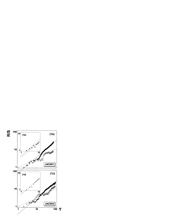
Figure 1: $R/S(y_{i},Y)$ as functions of $Y$ for given $y_{i}$’s; data are taken from Ref. 15 . For details see text.

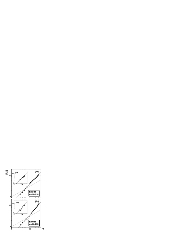
Figure 2: $R/S(y_{i},Y)$ as functions of $Y$ for given $y_{i}$’s. The results are taken from LAN et al. 16 . The broken lines indicate the $H=0.5$ case.

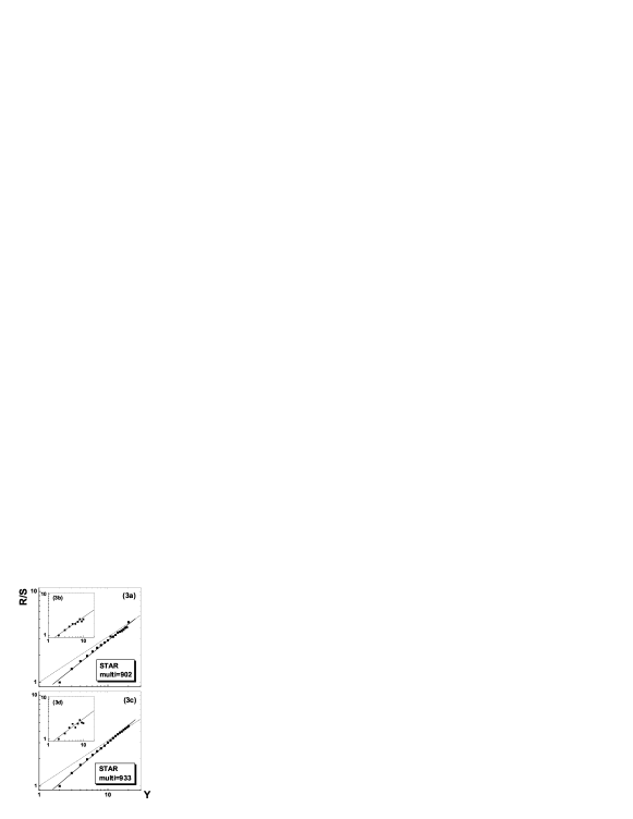
Figure 3: $R/S(y_{i},Y)$ as functions of $Y$ for given $y_{i}$’s. The results are taken from LAN et al. 16 . The broken lines indicate the $H=0.5$ case.

References

- (1) The theorctical scheme of such an approach can be found in textbooks. See e.g. Halzen and Martin, Quark and Leptons, and the references given therein.
- (2) See the following review articles and the references given therein. E.A. De Wolf, I.M. Dremin and W. Kittel, Phys. Reports, 270 1 (1996). S.P. Ratti, G. Salvadori, G. Gianini, S. Lovejoy, D. Schertzer, Z. Phys. C 61, 229 (1994). W. Kittel, Proceeding of the Second International Conference on Frontier Science, Sept 2003, Pavia, Italy, Physica A 228, 7 (2004).
- (3) H.D. Ursell, Proc. Camnb. Phil. Soc. 23, 685 (1927). J.E. Mayer and M.G. Mayer, Statistical Mechanics (John Wiley, New York, 1940) and the references given therein.
- (4) A. Bialas and R. Peschanski, Nucl. Phys. B 273, 703 (1986).
- (5) F. Takagi, Phys. Rev. Lett. 53, 427 (1984).
- (6) T. Ludlam and R. Slansky, Phys. ReV. D 12, 59 (1975).
- (7) T. Ludlam and R. Slansky, Phys. ReV. D 8, 1408 (1973).
- (8) Q. Liu and T. Meng, Phys. Rev. D 69, 054026 (2004).
- (9) B.B. Mandelbrot, Fractals and Scaling in Finance (Springer, 1997); and the references given therein.
- (10) B.B. Mandelbrot, Gaussian Self-Affinity and Fractals (Springer, 2002); and the references given therein.
- (11) B.B. Mandelbrot, The Fractal Geometry of Nature (Freeman, 1999).
- (12) H.E. Hurst, Trans. Am. Soc. Civ. Eng. 116, 770 (1951).
- (13) B.B. Mandelbrot & J.R. Wallis, Water Resources Research, 5, 967 (1969).
- (14) J. Feder, Fractals (Plenum Press, New York, 1988).
- (15) JACEE-Collaboration: T.H. Burnett et al., Phys. Rev. Lett. 50, 2062 (1983).
- (16) X. LAN, W. QIAN and X. CAI, Preprint: “Preconception-free analyses of high-multiplicity and large-flucatuation data for nucleus-nucleus collisions at different energy-ranges”, (submitted to HEP NP).
- (17) See e.g. R.E. Marshak, Conceptual Foundations of Modern Particle Physics (World Scientific, 1993) p. 284.