Large Mixing from Small:
Pseudo-Dirac Neutrinos and the Singular Seesaw

Abstract

If the sterile neutrino mass matrix in an otherwise conventional seesaw model has a rank less than the number of flavors, it is possible to produce pseudo-Dirac neutrinos. In a two-flavor, sterile rank 1 case, we demonstrate analytic conditions for large active mixing induced by the existence of (and coupling to) the sterile neutrino components. For the three-flavor, rank 1 case, “3+2” scenarios with large mixing also devolve naturally as we show by numerical examples. We observe that, in this approach, small mass differences can develop naturally without any requirement that masses themselves are small. Additionally, we show that significant three channel mixing and limited experimental resolution can combine to produce extracted two channel mixing parameters at variance with the actual values.

I Introduction

Conventional wisdom holds that neutrinos ought to be Majorana particles with very small masses, due to the action of a “seesaw” mechanismsee-saw , which is built on the concept of quark-lepton symmetryGSMcK . Alternatively, there have been theoretical suggestions regarding pseudo-Dirac neutrinos in the pastwolfm2 ; oldref , and again more recentlyGSMcK ; CHM ; othr , i.e., that neutrinos may well be Majorana particles occuring in nearly degenerate pairs. These can occur within the framework of the so-called “singular” see-saw where the rank of the mass matrix describing the (presumed to be) heavy neutrinos, which have no interactions (often referred to as “sterile” neutrinos) in the standard model (SM), is less than maximal.

Recent results from KamiokandesuperK on atmospheric neutrinos, from SudburySNO on solar neutrinos, and from KamLandKamL on long baseline reactor neutrinos, appear to require oscillations between nearly maximally mixed (active neutrino) mass eigenstates. Each of these analyses, however, argues that this mixing cannot be dominantly to sterile states such as are found in pseudo-Dirac pairs. On the other hand, the concatenation of the data from these experiments with that from LSNDLSND and other short baseline data does not appear to fit into a theoretical structure which only includes mixing among three active Majorana neutrinos. Many have therefore been motivated to consider the effects of additional (sterile, Majorana) neutrino states, the existence of which is accepted in the conventional “see-saw” extension of the SM, although there the actual states are generally precluded from appearing directly in experiments by an assumption that the masses of the sterile states are very large.

We investigate here how small flavor mixing effects in the sterile sector can lead to large mixing among active neutrinos in the presence of a singular see-saw. (In Ref.CHM , large mixing was achieved by means of a mass hierarchy in the Dirac mass sector.) Paralleling a convention in the quark sector, we assume the mass and flavor bases for the charged leptons are simultaneously diagonal, so that all flavor violations and oscillation phenomena are described as arising from the neutrino mixing angles alone.

It should be noted that there is no accepted principle that specifies the flavor space structure of the mass matrix assumed for the sterile sector. Some early discussionssee-saw ; wolfm2 implicitly assume that a mass term in the sterile sector should be proportional to the unit matrix. This has the pleasant prospect, in terms of the initial argument for the see-saw, that all active neutrino flavors have small masses on the scale of other fermions. However, since there is no obvious requirement that Dirac masses in the neutral lepton sector are the same as Dirac masses in any other fermionic sector, this result is not compelling. Indeed, Goldhaber has argued for a view of family structure and self-energy based masses that naturally produces small neutrino massesMaurice . We discuss here a more conventional possibility which arises from a minimal modification of the standard see-saw, namely that the rank of the mass matrix for the sterile sector is less than the number of flavors. Note that this does not conflict with quark-lepton symmetry which applies only to the number and character of states.

In this paper, which is an extension of referencehep , we shall concentrate on the case of a rank $1$ sterile matrix, relegating the rank $2$ case to some remarks at the end. (The analysis of short baseline data by Sorel, Conrad and ShaevitzSorel suggests that the rank $2$ case may not actually occur in Nature.) We note in passing that some Grand Unified Theories include more than $3$ fermions that are neutral under all of the interactions in the SM; a $4\times 4$ or larger, rank $1$ sterile mass matrix could lead to $3$ pseudo-Dirac pairs of neutrinos involving all of the active neutrinos of the SM.

Concentrating on a $3$-dimensional sterile space, we consider rank $1$ to be a natural case because whatever spontaneous symmetry breaking produces mass in that flavor space necessarily defines a specific direction. Before including the effects of the sterile mass, we assume three non-degenerate Dirac neutrinos, with Dirac masses, $m_{1}~{}<~{}m_{2}~{}<~{}m_{3}$, (although this is not essential,) which are each constructed from one Weyl spinor which is active under the $SU(2)_{W}$ of the SM and one Weyl spinor which is sterile under that interaction. (Being neutrinos, both Weyl fields have no interactions under the $SU(3)_{C}$ or the $U(1)$ of the SM.) There is then an MNS matrixMNS which relates these Dirac mass eigenstates to the flavor eigenstates in a manner completely parallel to that of the CKM matrixckm for quarks. Note, however, that these matrix elements are not the ones extracted directly from experiment, as the mass matrix in the sterile sector induces additional mixing.

We next use the Dirac mass ($m_{D}$) eigenstates to define bases in both the $3$-dimensional active flavor space and the $3$-dimensional sterile flavor spacefn1 . Following the spirit of the original see-saw, we exclude any initial Majorana mass term in the active space. If the Majorana mass matrix in the sterile space were to vanish also, the three flavors of Dirac neutrinos would be a mixture of (Dirac) mass eigenstates in a structure entirely parallel to that of the quarks.

A rank $1$ sterile mass matrix may be represented as a vector of length $M$ oriented in some direction in the $3$-dimensional sterile space. If that vector lies along one of the axes, then the Dirac neutrino that would have been formed from it and its active neutrino partner partake of the usual see-saw structure (one nearly sterile Majorana neutrino with mass approximately $M$ and one nearly purely active neutrino with mass approximately $m_{D}^{2}/M$) and the other two mass eigenstates remain Dirac neutrinos. If that vector lies in a plane perpendicular to one axis, the eigenstate associated with that axis will remain a pure Dirac neutrino, and the other two pairs of states form one pseudo-Dirac pair and a pair displaying the usual see-saw structure. Both of these pairs are mixtures of the $4$ Weyl fields associated with the two mixing Dirac neutrinos. In general, the structure consists of $2$ pseudo-Dirac pairs and one see-saw pair, all mixed.

As we implied above, the very large mixing required by the atmospheric neutrino measurements could have been taken to be evidence for a scheme involving pseudo-Dirac neutrinos. (This, after all, follows Pontecorvo’s initial suggestionBP .) However, pure mixing into the sterile sector is now strongly disfavorednsm . It is evident from the discussion above that there is a region of parameter space (directions of the vector) in which the two pseudo-Dirac pairs are very nearly degenerate, giving rise to the possibility of strong mixing in the active sector coupled with strong mixing into the sterile sector. We explore this point here.

The organization of the remainder of the paper is as follows: In the next section we discuss a two flavor, $4\times 4$ neutrino mass matrix analytically. In Sec.III, we present the general $6\times 6$ mass matrix and discuss the parameterization of the sterile mass matrix and various limiting cases. We show the spectrum for a general case. In Sec.IV, we apply our analysis to the case where the plane in question is perpendicular to the axis for the middle value ($m_{2}$) Dirac mass eigenstate, raising the possibility of near degeneracy between pseudo-Dirac pairs. Moving away from that plane produces large mixing amongst the members of those pseudo-Dirac pairs. In Sec.V, we show an example of the oscillation patterns that are produced and how limited experimental resolution can lead to errors in the extraction of physical parameters if the data analysis assumes only two channel mixing. Finally, we remark on the structures expected for a rank $2$ sterile matrix and then reiterate our conclusions.

II Two flavor case

In our examination of the consequences of assuming a rank $1$ mass matrix in the sterile subspace, we will show below that there are certain parameter ranges for which there is very large mixing induced in the active subspace, even though there is no explicit mixing among the original Dirac bispinors. To see how this arises, it is useful to look at the two flavor model for which we can obtain an analytic description of the mass eigenvalues as a power series in $\frac{1}{M}$. We then can find the eigenfunctions, again as a power series in $\frac{1}{M}$, and look at the ratio of the coefficients for the two active components. We examine the conditions which allow for large active mixing when there is no mixing in the original Dirac space.

In the next section we shall discuss the case where two pseudo-Dirac pairs are nearly degenerate and follow the mixing patterns as we move away from that region of parameter space. To facilitate that discussion, we explore this subsystem where analytic approximations are available, i.e., the limit where one Dirac mass eigenstate remains uncoupled from all of the other states. Anticipating the following section, we decouple what is there $m_{2}$. That is, we examine a two flavor system in which the Dirac mass eigenvalues are $m_{1}$ and $m_{3}$.

It is useful to define:

$$m_{0}^{2} = m_{1}^{2}\cos^{2}\theta+m_{3}^{2}\sin^{2}\theta$$ (1)

$$a = \frac{\left(m_{1}^{2}-m_{3}^{2}\right)\sin\theta\cos\theta}{m_{0}\sqrt{2}}$$ (2)

$$b = \frac{m_{1}m_{3}}{m_{0}}$$ (3)

and $c=\cos\theta$, $s=\sin\theta$. Note the additional $1/\sqrt{2}$ factor in $a$. These refer to the mass matrix

$${\cal{M}}_{1}=\left(\begin{array}[]{cccc}0&0&m_{1}&0\\ 0&0&0&m_{3}\\ m_{1}&0&Ms^{2}&Mcs\\ 0&m_{3}&Mcs&Mc^{2}\end{array}\right)$$ (4)

where $m_{1},m_{3}$ are Dirac masses for the two neutrino flavors and $M$ is the single nonzero mass eigenvalue in the sterile sector. The angle $\theta$ defines the deviation of the direction in the sterile subspace of the eigenvector for this nonzero mass from one of the flavor axes defined by the Dirac mass eigenstates. Note that the structure in Eq.(4) is equivalent to the assumption that the MNSMNS analog of the CKMckm matrix for the quarks is the unit matrix.

It is useful to transform ${\cal{M}}_{1}$ into the form

$$\cal{M}=\left(\begin{array}[]{cccc}m_{0}&0&0&a\\ 0&-m_{0}&0&-a\\ 0&0&0&b\\ a&-a&b&M\end{array}\right)$$ (5)

in order to see that, to lowest order, the three small eigenvalues are $\pm m_{0},0$. (Note the minus sign on the $a$ in the (2,4) and (4,2) positions.) The matrix effecting the transformation ${\cal{M}}=\Omega^{{\dagger}}{\cal{M}}_{1}\Omega$ is

$$\Omega=m_{0}^{-1}\left(\begin{array}[]{cccc}m_{1}s/\sqrt{2}&-m_{1}s/\sqrt{2}&m_{3}c&0\\ -m_{3}c/\sqrt{2}&m_{3}c/\sqrt{2}&m_{1}s&0\\ m_{0}s/\sqrt{2}&m_{0}s/\sqrt{2}&0&m_{0}c\\ -m_{0}c/\sqrt{2}&-m_{0}c/\sqrt{2}&0&m_{0}c\end{array}\right)$$ (6)

This suggests writing the characteristic equation as:

$$\mu\left(m_{0}^{2}-\mu^{2}\right)\mu(M-\mu)=2\mu^{2}a^{2}-\left(m_{0}^{2}-\mu^{2}\right)b^{2}$$ (7)

which is convenient for iterative solution in a series in $M^{-1}$. The usual equation obtained directly from $\left|{\cal{M}}_{1}-\mu\right.$ 1$\left.\right|=0$,

$$\mu^{4}-\mu^{3}M-\mu^{2}\left(m_{1}^{2}+m_{3}^{2}\right)+\mu m_{0}^{2}M+m_{1}^{2}m_{3}^{2}=0,$$ (8)

is just the same equation.

The solutions to order $M^{-2}$ are

$$\mu_{1} = m_{0}-\frac{a^{2}}{M}-\frac{a^{2}}{m_{0}M^{2}}\left(m_{0}^{2}-\frac{a^{2}}{2}-b^{2}\right)$$ (9)

$$\mu_{2} = -m_{0}-\frac{a^{2}}{M}+\frac{a^{2}}{m_{0}M^{2}}\left(m_{0}^{2}-\frac{a^{2}}{2}-b^{2}\right)$$ (10)

$$\mu_{3} = -\frac{b^{2}}{M}+{\cal O}(M^{-3})$$ (11)

$$\mu_{4} = M+\frac{b^{2}}{M}+2\frac{a^{2}}{M}+{\cal O}(M^{-3})$$ (12)

Notice that the eigenvalues sum to $M$ as they must and that the $\pm m_{0}$ eigenvalues are shifted in opposite directions at $O(M^{-2})$ but in the same direction at $O(M^{-1})$, which is a small amount for sufficiently large $M$. The latter shift is why these form a pseudo-Dirac pair rather than simply a Dirac bispinor. Note also that $\mu_{3}$ and $\mu_{4}$, do not acquire $O(M^{-2})$ corrections; their next correction is at the next higher order.

Having obtained the eigenvalues, we now solve for the eigenvectors. Since our interest is in the mixing in the active sector, it is useful to carry this exercise out in the original representation, that of ${\cal{M}}_{1}$. In this representation, we define the $i^{th}$ eigenvector as

$$\phi_{i}=\left(\begin{array}[]{c}\alpha_{i}\\ \beta_{i}\\ \gamma_{i}\\ \delta_{i}\end{array}\right),$$ (13)

where $\alpha_{i}$ and $\beta_{i}$ are the two active components and $\gamma_{i}$ and $\delta_{i}$ are the two sterile components.

Picking three equations, we find

$$-\mu_{i}\alpha_{i}+m_{1}\gamma_{i} = 0$$

$$-\mu_{i}\beta_{i}+m_{3}\delta_{i} = 0$$

$$m_{3}\beta_{i}+Msc\gamma_{i}+(Mc^{2}-\mu_{i})\delta_{i} = 0$$ (14)

A number of points are immediately clear from Eqs.(14): Since $\mu_{4}\sim M$, $\beta_{4}$ and $\alpha_{4}$ are small (${\cal O}(m_{D}/M)$) so the fourth eigenstate is almost entirely decoupled from the active sector. Conversely, since $\mu_{3}\sim{\cal O}(m_{D}^{2}/M)$, $\gamma_{3}$ and $\delta_{3}$ are small (${\cal O}(m_{D}/M)$) so the third eigenstate resides almost entirely in the active sector. Finally, since $\mu_{1}$ and $\mu_{2}$ are of order ${\cal O}(m_{D})$, $\gamma_{1,2}$ and $\delta_{1,2}$ are comparable with $\beta_{1,2}$ and $\alpha_{1,2}$ so these two eigenstates are generally strongly mixed between the active and sterile sectors, i.e., they form a pseudo-Dirac pair.

Substituting for $\gamma_{i}$ and $\delta_{i}$ gives an equation for the ratio

$$\frac{\beta_{i}}{\alpha_{i}} = -\frac{M\mu_{i}sc}{[\mu_{i}(Mc^{2}-\mu_{i})+m_{3}^{2}]}$$ (15)

$$= -\frac{sc}{[c^{2}-\frac{\mu_{i}}{M}+\frac{m_{3}^{2}}{M\mu_{i}}]}.$$

Note that if either $s=0$ or $c=0$, one pair of states forms a purely Dirac bispinor and the other becomes the usual see-saw pair of Majorana states.

For the light mass eigenstates, the ratio $\beta_{i}/\alpha_{i}$ is a measure of mixing in the active sector. Solving Eq.(15), we find that

$$|\frac{\beta_{1}}{\alpha_{1}}|\,\,\,=|\frac{\beta_{2}}{\alpha_{2}}|\,\,\,=|\frac{\alpha_{3}}{\beta_{3}}|\,\,\,=\frac{m_{3}}{m_{1}}{\rm tan}(\theta),$$ (16)

where the last equality is correct to ${\cal O}(m_{D}^{2}/M^{2})$ and the first two are correct to ${\cal O}(m_{D}/M)$. It is apparent that, in all three states, the mixing of the active components can be large simultaneously.

Turning back to the amplitudes of the sterile components, we see from the first two lines of Eq.(14) that

$$\frac{\gamma_{i}}{\alpha_{i}} = \frac{\mu_{i}}{m_{1}}$$

$$\frac{\delta_{i}}{\beta_{i}} = \frac{\mu_{i}}{m_{3}}.$$ (17)

Hence, for a large range of values of ($m_{1}$, $m_{3}$, $\theta$), these ratios are ${\cal O}(1)$ for $i=1$ and $2$, which is, of course, characteristic of a pseudo-Dirac pair. As long as $M$ is large, $\gamma$, $\delta$ are small for $i=3$ since $\mu_{3}\sim 0$, and huge for $i=4$ since $\mu_{4}\sim M$. This reiterates the fact that the massive sterile state is quite decoupled, while the light sterile can be strongly coupled into the active states and the pseudo-Dirac states significantly mixed across all four components.

Thus, in this simple, two flavor model, we have demonstrated that a misalignment of the direction vector for the heavy sterile mass with the axes determined by the Dirac mass eigenstates necessarily induces mixing in the active sector for all of the light Majorana mass eigenstates, even with a unit MNS matrix for the Dirac mass matrix. This point has been raised previously in Ref.rabi in a different context.

Moreover, large mixing of active states results over a region of the $(m_{1},m_{3},\theta)$ parameter space where the mass ratio and the deviation angle of the sterile components from flavor alignment approximately compensate, i.e., near the line determined by setting the rightmost quantity in Eq.(16) to one. Mixing in the Dirac sector by an MNS matrix should not alter the general feature of achieving large mixing ”naturally”.

Finally, we note explicitly the difference in oscillation structure between this $4\times 4$ neutrino mass matrix and the $2\times 2$ Majorana (or Dirac) mixing usually applied to interpret experiments. As shown by Eqs.(3) or Eqs.(9, 10, 11), instead of one mass difference, here

there are at least two independent mass differences, even in the limit of large sterile mass ($M$). Thus, simple two channel analyses are not guaranteed to extract the true physical oscillation parameters from experimental results. This problem is exacerbated in the $6\times 6$ case that we discuss in the next Section, in which at least four independent mass differences appear where it has been conventionally assumed that there can only be two.

III General mass matrix

The flavor basis for the active neutrinos and the pairing to sterile components defined by the (generally not diagonal) Dirac mass matrix could be used to specify the basis for the sterile neutrino mass matrix, $M_{S}$. Instead we take the basis in the $3\times 3$ sterile subspace to allow the convention described below. This implies a corresponding transformation of the Dirac mass matrix, which is irrelevant at present since the entries in that matrix are totally unknown.

We define our convention for the choice of axes in the $3\times 3$ sterile subspace as follows. Denote the nonzero mass eigenvalue of the rank $1$ by $M$ and choose its eigenvector initially in the third direction. Then rotate this vector, first by an angle of $\theta$ in the $1-3$ plane and then by $\phi$ in the $1-2$ plane. The rotation is chosen so that the Dirac mass matrix which couples the active and sterile neutrinos becomes diagonal, i.e., the basis is defined by Dirac eigenstates. This produces a $3\times 3$ mass matrix in the sterile sector denoted by

$$M_{S}=M\left[\begin{array}[]{ccc}\cos^{2}\phi\sin^{2}\theta&\cos\phi\sin\phi\sin^{2}\theta&\cos\phi\sin\theta\cos\theta\\ \cos\phi\sin\phi\sin^{2}\theta&\sin^{2}\phi\sin^{2}\theta&\sin\phi\sin\theta\cos\theta\\ \cos\phi\sin\theta\cos\theta&\sin\phi\sin\theta\cos\theta&\cos^{2}\theta\end{array}\right].$$ (18)

In this representation, the Dirac mass matrix is diagonal by construction

$$m_{D}=\left[\begin{array}[]{ccc}m_{1}&0&0\\ 0&m_{2}&0\\ 0&0&m_{3}\end{array}\right].$$ (19)

Note that there are special cases. For $\theta=0$ and any value for $\phi$,

$$M_{S}=\left[\begin{array}[]{ccc}0&0&0\\ 0&0&0\\ 0&0&M\end{array}\right].$$ (20)

For $\theta=\pi/2$ and $\phi=0$,

$$M_{S}=\left[\begin{array}[]{ccc}M&0&0\\ 0&0&0\\ 0&0&0\end{array}\right],$$ (21)

and, for $\theta=\pi/2$ and $\phi=\pi/2$,

$$M_{S}=\left[\begin{array}[]{ccc}0&0&0\\ 0&M&0\\ 0&0&0\end{array}\right].$$ (22)

These are equivalent under interchanges of the definition of the third axis.

The $6\times 6$ submatrixfn2 of the full $12\times 12$ is, in block form,

$${\cal M}=\left[\begin{array}[]{cc}0&m_{D}\\ m_{D}&M_{S}\end{array}\right].$$ (23)

Since we are ignoring CP violation here, no adjoints or complex conjugations of the mass matrices appear.

Note that, in the chiral representation, the full $12\times 12$ matrix is

$$\left[\begin{array}[]{cc}0&{\cal M}\\ {\cal M}&0\end{array}\right].$$

Thus the full set of eigenvalues will be $\pm$ the eigenvalues of ${\cal M}$. Where it matters for some analysis we keep track of the signs of the eigenvalues, however for most results we present positive mass eigenvalues.

After some algebra, we obtain the secular equation

$$0 = \lambda^{6}-M\lambda^{5}-(m_{1}^{2}+m_{2}^{2}+m_{3}^{2})\lambda^{4}$$

$$+M[m_{3}^{2}\sin^{2}\theta+m_{2}^{2}(\sin^{2}\theta\cos^{2}\phi+\cos^{2}\theta)]\lambda^{3}$$

$$+(m_{1}^{2}m_{2}^{2}+m_{2}^{2}m_{3}^{2}+m_{3}^{2}m_{1}^{2})\lambda^{2}$$

$$-M(m_{1}^{2}m_{2}^{2}\cos^{2}\theta+m_{2}^{2}m_{3}^{2}\cos^{2}\phi\sin^{2}\theta$$

$$+m_{3}^{2}m_{1}^{2}\sin^{2}\phi\sin^{2}\theta)\lambda$$

$$-m_{1}^{2}m_{2}^{2}m_{3}^{2}.$$

This may be rewritten as

$$0 = (\lambda^{2}-m_{1}^{2})(\lambda^{2}-m_{2}^{2})(\lambda^{2}-m_{3}^{2})$$

$$-\lambda M\left(\lambda^{4}-\left[m_{3}^{2}\sin^{2}\theta+m_{2}^{2}(\sin^{2}\theta\cos^{2}\phi+\cos^{2}\theta)\right.\right.$$

$$\left.\left.+m_{1}^{2}(\sin^{2}\theta\sin^{2}\phi+\cos^{2}\theta)\right]\lambda^{2}\right.$$

$$\left.+m_{1}^{2}m_{2}^{2}\cos^{2}\theta+m_{2}^{2}m_{3}^{2}\sin^{2}\theta cos^{2}\phi\right.$$

$$\left.+m_{3}^{2}m_{1}^{2}\sin^{2}\theta\sin^{2}\phi\right).$$

The special cases follow directly. For $\theta=0$, we find

$$(\lambda^{2}-m_{1}^{2})(\lambda^{2}-m_{2}^{2})(\lambda^{2}-M\lambda-m_{3}^{2})=0,$$ (26)

for $\theta=\pi/2$ and $\phi=0$

$$(\lambda^{2}-m_{2}^{2})(\lambda^{2}-m_{3}^{2})(\lambda^{2}-M\lambda-m_{1}^{2})=0,$$ (27)

and for $\theta=\pi/2$ and $\phi=\pi/2$

$$(\lambda^{2}-m_{3}^{2})(\lambda^{2}-m_{1}^{2})(\lambda^{2}-M\lambda-m_{2}^{2})=0.$$ (28)

If $m_{1}^{2}=m_{2}^{2}=m_{3}^{2}=m^{2}$, then we find

$$(\lambda^{2}-m^{2})^{2}(\lambda^{2}-M\lambda-m^{2})=0.$$ (29)

Due to the wide range of possibilities inherent in the system, it is useful to examine specific numerical examples. For the immediate exercise, we have picked the following parameters: $m_{1}=1$, $m_{2}=2$, $m_{3}=3$ and $M=1000$. The relatively small value of $M$ is chosen so that the splittings are not so tiny as to be difficult to discern.

For this choice, the eigenvalues have a definite pattern for all values of $\theta$ and $\phi$. There are two very close pairs, with mass eigenvalues between $1$ and $3$. There is one very small eigenvalue, of order $10^{-3}$ reflecting the ratio of $m_{D}$ to $M$, and one large eigenvalue of order $10^{3}$ (i.e., of order $M$). Treating the last two as a pair despite their disparity in mass allows us to present results in tabular form, one for each pair, for sets of angles $\theta,\phi=\pi/8,\pi/4,3\pi/8$.

First, for the lower mass close pair, we have

$$\begin{array}[]{lccc}\theta\backslash\phi&\pi/8&\pi/4&3\pi/8\\ &&&\\ \pi/8&1.398125&1.230175&1.068477\\ &1.394934&1.228025&1.067688\\ &&&\\ \pi/4&1.809478&1.478863&1.151936\\ &1.808183&1.477134&1.150941\\ &&&\\ 3\pi/8&1.877166&1.562977&1.18999\\ &1.876742&1.561911&1.189146\end{array}$$ (30)

Then, for the next mass pair with close eigenvalues, we find

$$\begin{array}[]{lccc}\theta\backslash\phi&\pi/8&\pi/4&3\pi/8\\ &&&\\ \pi/8&2.038992&2.107688&2.158044\\ &2.038729&2.107156&2.157407\\ &&&\\ \pi/4&2.347974&2.46348&2.529128\\ &2.346047&2.462176&2.52809\\ &&&\\ 3\pi/8&2.816525&2.847539&2.868607\\ &2.815691&2.846972&2.868186\end{array}$$ (31)

Finally, even though it does not directly impact the argument, we display the remaining pair in order to present a complete set.

$$\begin{array}[]{lccc}\theta\backslash\phi&\pi/8&\pi/4&3\pi/8\\ &&&\\ \pi/8&1000.008&1000.008&1000.008\\ &0.00444&0.005366&0.006778\\ &&&\\ \pi/4&1000.005&1000.006&1000.006\\ &0.001997&0.002717&0.004248\\ &&&\\ 3\pi/8&1000.003&1000.003&1000.004\\ &0.001289&0.001819&0.003092\end{array}$$ (32)

IV Two nearly degenerate pseudo-Dirac pairs

Applying the techniques of the last section, we find the angle $\theta$ such that $m_{2}$ and the eigenvalue for the pseudo-Dirac pair above, $m_{0}$, are approximately degenerate. We then vary $\phi$ away from $0$ and display the eigenfunctions. To illustrate the general nature of the result, we have changed the Dirac masses from the even spacing used above.

In Table I, the Dirac masses are taken to be $m_{1}=1$, $m_{2}=1.1$, and $m_{3}=3$. The value for $m_{2}$ has been changed from above so that we can demonstrate that small angles in the sterile sector can lead to large mixing in the active sector. Again, in order to display the structure of the spectrum, we have chosen $M=1000$, rather than a larger value, expected to be more realistic, but which would suppress the difference scale between the pairs. The angles are given in degrees.

Table I represents only a small part of the available parameter space; the values of the angles are chosen to display some interesting possible features. First, $\theta$ has been chosen so that, at $\phi=0$, the Dirac pair at $m_{2}$ is bracketed by the pseudo-Dirac pair. Such a value of $\theta$ exists for any pattern of the Dirac masses. Then, for small values of $\phi$, there are always two nearly degenerate pseudo-Dirac pairs.

Note that, for $\phi=0$, there is no mixing between the field labelled by $2$ and the remaining fields, while for the next entry at $\phi=2.25$ degrees there is considerable mixing. That mixing increases with $\phi$ as the difference bewteen the eigenvalues increases. The pattern described by the centroids of the pseudo-Dirac pairs is fixed by the angles $\theta$ and $\phi$. If $M$ is increased, that pattern hardly changes. The primary effect of increasing $M$, consistent with the analysis in Sec.II, is to decrease the separation of the two members of each pseudo-Dirac pair while producing the usual see-saw behavior for the remaining pair. Thus, tiny differences in mass between masses that are not especially small themselves, are, in the usual sense of the term, natural in this approach.

The implication for oscillation phenomena is clear. A given weak interaction produces an active flavor eigenstate which is some linear combination of the three active components listed in Table I. That then translates into a linear combination of the six mass eigenstates. From Table I, it is clear that the involvement of the heavy Majorana see-saw state is minimal, so the system effectively consists of the light Majorana see-saw state and the four Majorana states arising from the two pseudo-Dirac pairs. These five states include all three active neutrinos, generating a natural 3+2 scenario.

Since these five mass eigenstates have both active and sterile components, the subsequent time evolution will involve both flavor changing oscillations and oscillation into (and back out of) the sterile sector. This can lead to very complex oscillation patterns, as there are $10$ mass differences, $4$ of which are independent. A specific example is discussed in the next section.

Finally, inspection of the column labelled “1active” for $\phi=2.25$ or $\phi=4.5$, for example, shows that the presence of a rank $1$ sterile mass matrix can seriously change any mixing pattern of the MNS typeMNS , from that which would have obtained with purely Dirac neutrinos.

V example

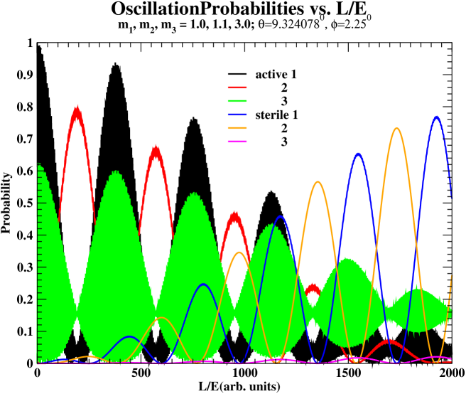
Figure 1: Oscillations for all six channels commencing from one active flavor with appearance probabilities for the two other actives and the steriles using the second set of angle parameters in Table I.

In Figs.1 to 3, we plot the oscillation patterns that appear for the parameters set by the second entry in Table I. Fig.1 gives an overview of the case where an active neutrino (labelled $1$) is produced initially. The plot is given versus $L/E$, where $L$ is the distance from the neutrino source and $E$ is the energy (bin) of the neutrino observed. (As shown in the Appendix, $L/p$, where $p$ is the momentum of the neutrino, might well be the more correct variable to use, but the difference is certainly irrelevant in all conceivable neutrino experiments.)

The (compressed scale) Fig.1 shows rapid oscillations between active neutrinos $1$ and $3$ with a later appearance of the active neutrino $2$. Note the large mixing among all three channels of active neutrinos. The mixing to sterile neutrinos is large also, but occurs on a much larger $L/E$ scale, corresponding to the much smaller mass difference (approximate degeneracy) of the pseudo-Dirac pairs.

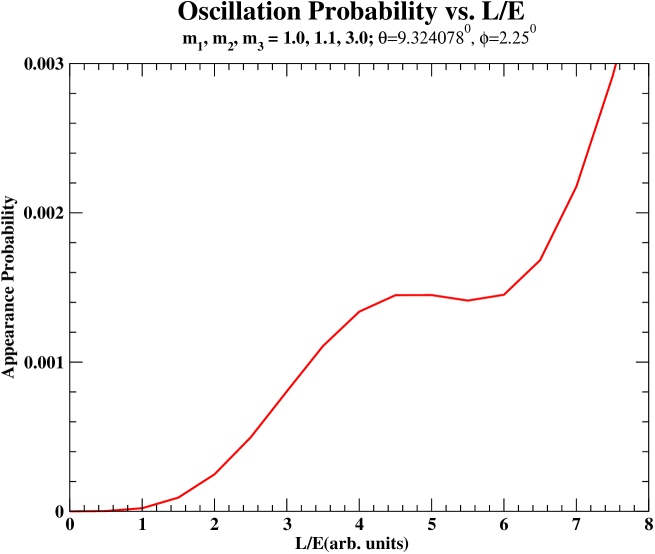
Figure 2: Appearance probability for one neutrino flavor using the second set of angle parameters in Table I. The arbitrary units of the abscissa may be viewed as time in the rest frame or $L/E$ in the laboratory. See Appendix.

Fig.2 extracts from Fig.1 the appearance of active neutrino $2$ at small $L/E$ (short baseline experiments). Clearly, attempting to fit this highly nonsinusoidal behavior with two channel sinusoidal mixing will generally not yield physical mixing parameters in good agreement with the actual three channel case.

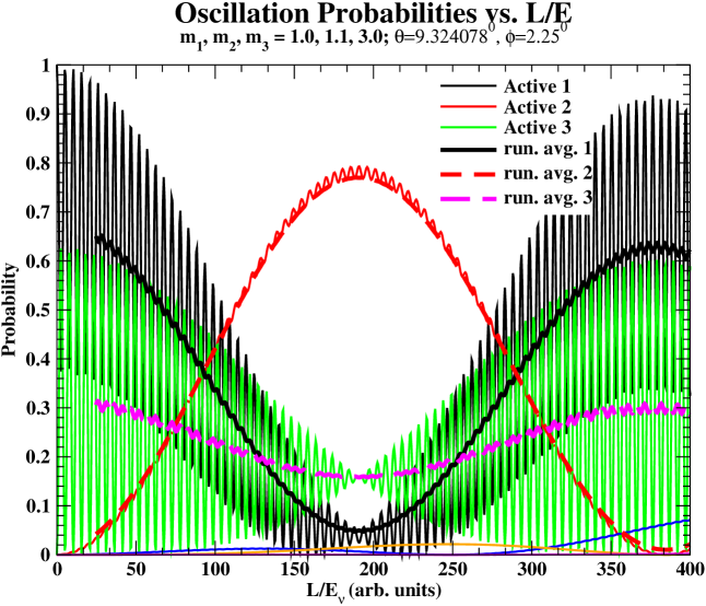
Figure 3: Effects of limited resolution in $L/E$. Running averages over 100 units have been taken for each of the active curves. (The curves for the sterile neutrinos remain as in Fig.1.)

Fig.3 emphasizes how such an error may be magnified by limited resolution in an experiment. The heavy black curve is the average over 100 $L/E$ units of the probability for finding the initial neutrino flavor. It approximates the shape of the envelope of the high frequency oscillations. A two channel analysis would clearly find a small difference between the squared masses for the mixing from active neutrino $1$ to active neutrino $3$ despite the obviously larger value demonstrated by the rapid oscillation cycles. A similar conclusion follows from the cycle-averaged curve for appearance of active neutrino $3$. Finally, one would be tempted to conclude that the mixing to active neutrino $2$ is small or negligible, when in fact it is about as large as any other mixing in the full case.

Labelling active neutrino $1$ as the muon neutrino, active neutrino $3$ as the tau neutrino and active neutrino $2$ as the electron neutrino illustrates our concerns about the strong conclusions drawn from atmospheric and accelerator neutrino experiments by means of two channel mixing analyses. Similar concernstw have also been raised in the literature previously.

VI Rank $2$

We have not discussed the case of rank $2$ matrices explicitly, although the pattern is obvious. In such a case, there would be two see-saw pairs and one pseudo-Dirac pair, leading to three active and one sterile light neutrino. While this pattern has been analyzed in the literature, we do not find any compelling pattern for it in the sterile sector. Furthermore, the current consistency of all neutrino oscillation data can be accomodated much more easily (and perhaps only, as indicated by Ref.Sorel ,) in the rank $1$ case discussed in this paper. Therefore we do not discuss rank $2$ at this time.

VII Conclusions

We have considered here the effects on neutrinos in the SM of the recurrently successful and conventional constraint of quark-lepton symmetry, namely, the existence of six independent Weyl spinor fields of neutrinos, three corresponding to active and three corresponding to sterile neutrinos. In the now venerable see-saw approach, the latter three effectively disappear from the excitation spectrum, leaving small Majorana masses for the active states as a residuum. We have examined the effect on this system of a rank less than three character of the $3\times 3$ mass matrix in the sterile sector and studied the rank $1$ case, in particular.

In the rank $1$ case on which we have focused, we find that the neutrino fields naturally form into two pseudo-Dirac pairs, leaving only one almost pure Majorana active neutrino and one conventionally very heavy sterile Majorana neutrino. More importantly, we also find a naturally strong mixing between the active and sterile parts of the two pseudo-Dirac pairs. Further, we find that this can easily affect the mixing between active neutrinos even if it is otherwise small. That is, even if the Dirac mass matrix induced mixing analogous to what is known to occur in the quark sector is small or absent, mixing between active neutrinos can develop with large values. In a two flavor case, we demonstrated analytically that this strong mixing can develop over a wide range of parameters.

We have chosen a limited relative value of the sterile neutrino mass scale, $M$, that allows for easy discernment of the nature of the effects. It should be noted, however, that the primary effect of increasing $M$ is to decrease the separation of the two members of each pseudo-Dirac pair while producing the usual see-saw behavior for the remaining pair. Thus, tiny differences in mass between masses that are not especially small themselves are, in the usual sense of the term, natural in this approach. This is contrary to the general expectation that the small mass differences responsible for the observed neutrino oscillation phenomena presage small absolute masses for all of the neutrinos. Furthermore, increasing the value of $M$ without altering the Dirac masses retains the features and scales of the oscillations essentially unchanged; the only significant change is that the appearance of the sterile components is delayed to even greater values of $L/E$.

The features described above are most easily discerned in the case when the Dirac mass terms for the neutrinos are well separated in value. It remains conceivable that, if their differences are small for some other reason, then the splitting between the pseudo-Dirac pairs may be larger than that between flavors. In this case, it is still true that large flavor mixing is naturally induced.

Finally, we presented a specific model which raises concerns about the conclusions drawn from analyses of neutrino oscillation experiments in terms of two channel mixing: Such analyses may be misleading regarding the true values of physical parameters. After the completion of this work, we learned of papersernst which have independently suggested that such a concern may well be justified.

VIII Acknowledgments

This research is supported in part by the Department of Energy under contract W-7405-ENG-36, in part by the National Science Foundation under NSF Grant # PHY0099385 and in part by the Australian Research Council.

IX APPENDIX: Two Mass Eigenstate Oscillations

There has been some confusion and discussion in the literature regarding the space and time dependence of neutrino oscillations. We briefly present here an argument in the rest frame of a state of a given flavor that demonstrates the time dependence unequivocally. By boosting the observer instead of the state, we demonstrate the equivalence of the usual $L/E_{\nu}\approx L/p_{\nu}$ dependence, derived in several ways, to the time dependence in the rest frame. Hence the figures in the main sections of this paper can be viewed as either variation with $L/E_{\nu}$, $L/p_{\nu}$ or time.

We begin with a flavor eigenstate composed of two different mass eigenstate contributions, in their common rest frame. Let

$$c\equiv cos(\theta) s\equiv sin(\theta)$$ ;

$$|\nu_{f}> = \;\;\,c\,|\nu_{1}>+s\,|\nu_{2}>$$

$$|\nu_{g}> = -s\,|\nu_{1}>+c\,|\nu_{2}>$$ (33)

to fix conventions for neutrino flavors $f$ and $g$ composed in two channel mixing from neutrino mass eigenstates $\nu_{1}$ with mass $m_{1}$ and $\nu_{2}$ with mass $m_{2}$. The time evolution of the state initially in flavor $f$ in this common rest frame is given by

$$|\nu(t)>=e^{-\imath{\bf H}t}\,|\nu(0)\equiv\nu_{f}>$$ (34)

$$= c\,e^{-\imath m_{1}t}|\nu_{1}>+s\,e^{-\imath m_{2}t}|\nu_{2}>$$

The probability of appearance of ${\nu}_{g}$ from the ${\nu}_{f}$ source is given by

$$|<\nu_{g}|\nu(t)>|^{2}=|e^{-\imath\frac{(m_{1}+m_{2})t}{2}}|^{2}$$ (35)

$$\times c^{2}s^{2}\,|-e^{\imath\frac{(m_{2}-m_{1})t}{2}}+e^{-\imath\frac{(m_{2}-m_{1})t}{2}}|^{2}$$

$$= sin^{2}(2\theta)\,sin^{2}(\frac{\Delta m\,t}{2})$$

Viewed from a frame moving past these states with velocity $\beta$, the relation between position $L$ in the moving frame and the time is affected both by the velocity and by time dilatation, i.e.,

$$t=L/[{\beta\gamma}]\sim Lm_{{av}}/p_{{\nu}},$$ (36)

where we choose the motion of the frame to be consistent with the ratio of the average neutrino mass and mean neutrino momentum. Hence

$$|<\nu_{g}|\nu(t)>|^{2}\sim sin(2\theta)\,sin^{2}({\Delta m^{2}}L/[4p_{{\nu}}])$$ (37)

As usual, the units are determined by the relation

$${1.27}\frac{\Delta m^{2}}{eV^{2}}\frac{L_{osc}}{km}\frac{GeV/c}{p_{\nu}}=\pi$$ (38)

consistent with all conventional analyses and expectations.

It should be noted that different energy (mass) eigenstates do not interefere with each other. The effect derives entirely from the independent phase advance of the individual states and their translation relative to the laboratory rest frame.

TABLE I: Eigenmasses for various values of $\theta$ and $\phi$ for cases of two approximately degenerate pseudo-Dirac pairs.

__________________________________________________________________________

$\theta=9.324078$, $\phi=0$

      mass     1active    2active   3active  1sterile  2sterile  3sterile

   1.099328   0.635032   0.000000 -0.310533  0.698108  0.000000 -0.113793
   1.100680  -0.633620   0.000000  0.314383  0.697413  0.000000 -0.115345
   1.100000   0.000000   0.707107  0.000000  0.000000  0.707107  0.000000
   1.100000   0.000000  -0.707107  0.000000  0.000000  0.707107  0.000000
   0.007438   0.441883   0.000000  0.897064 -0.003287  0.000000 -0.002224
1000.008789   0.000162   0.000000  0.002960  0.162017  0.000000  0.986784

$\theta=9.324078$, $\phi=2.25$

      mass     1active    2active    3active  1sterile  2sterile  3sterile

   1.095953   0.479130  -0.468214  -0.225940  0.525106 -0.466489 -0.082539
   1.096608   0.437964  -0.514829  -0.208027 -0.480274  0.513243  0.076041
   1.103359   0.416946   0.529767  -0.212981  0.460041  0.531383 -0.078333
   1.104056  -0.458049  -0.484588   0.235669  0.505710  0.486376 -0.086730
   0.007438   0.441553   0.015769   0.897088 -0.003285 -0.000109 -0.002224
1000.008789   0.000162   0.000007   0.002960  0.161892  0.006361  0.986784

$\theta=9.324078$, $\phi=4.5$

      mass     1active    2active    3active  1sterile  2sterile  3sterile

   1.092254   0.479875  -0.471453  -0.217491  0.524155 -0.468127 -0.079183
   1.092888  -0.458763   0.495815   0.209390  0.501371 -0.492614 -0.076279
   1.107010   0.416602   0.526536  -0.221472  0.461189  0.529886 -0.081725
   1.107726   0.437718   0.503654  -0.234323 -0.484866 -0.507196  0.086521
   0.007439   0.440571   0.031517   0.897156 -0.003273 -0.000217 -0.002226
1000.008789   0.000162   0.000014   0.002960  0.161517  0.012712  0.986784

$\theta=9.324078$ $\phi=22.5$

      mass     1active    2active    3active  1sterile  2sterile  3sterile

   1.062925   0.550356  -0.405921  -0.179528  0.584987 -0.392239 -0.063608
   1.063381   0.546548  -0.411257  -0.179609 -0.581185  0.397574  0.063663
   1.134871   0.337840   0.568726  -0.249457  0.383405  0.586755 -0.094367
   1.135731   0.341702   0.564710  -0.254038 -0.388074 -0.583058  0.096172
   0.007475   0.409265   0.154109   0.899298 -0.003058 -0.001048 -0.002241
1000.008789   0.000150   0.000068   0.002960  0.149684  0.062001  0.986784

$\theta=9.324078$ $\phi=45$

      mass     1active    2active    3active  1sterile  2sterile  3sterile

   1.030458   0.632073  -0.290233  -0.127244  0.651329 -0.271878 -0.043708
   1.030692  -0.630801   0.292859   0.127989  0.650162 -0.274406 -0.043972
   1.163620   0.226485   0.612428  -0.270973  0.263544  0.647849 -0.105102
   1.164612   0.227955   0.610618  -0.274587 -0.265472 -0.646488  0.106595
   0.007566   0.315141   0.286490   0.904762 -0.002384 -0.001969 -0.002282
1000.008789   0.000115   0.000126   0.002960  0.114563  0.114563  0.986784
________________________________________________________________________

References

- (1) M. Gell-Mann, P. Ramond and R. Slansky, in Supergravity, Proceedings of the Workshop, Stony Brook, New York, 1979, ed. by P. van Nieuwenhuizen and D. Freedman (North-Holland, Amsterdam, 1979), p. 315; T. Yanagida, in Proceedings of the Workshop on the Unified Theories and Baryon Number in the Universe, Tsukuba, Japan, 1979, edited by O. Sawada and A. Sugamoto (KEK Report No. 79-18, Tsukuba, 1979), p.95; R.N. Mohapatra and G. Senjanovic, Phys. Rev. Lett. 44 (1980) 912; S.L. Glashow, in Quarks and Leptons, Cargese (July 9-29, 1979), eds. M. Levy et al. (Plenum, 1980, New York), p. 707.
- (2) T. Goldman, G.J. Stephenson Jr. and B.H.J. McKellar, Mod. Phys. Lett. A15 (2000) 439; nucl-th/0002053.
- (3) L. Wolfenstein, Phys. Lett. B107 (1981) 77; Nucl. Phys. B186 (1981) 147.
- (4) M. Kobayashi, C.S. Lim and M.M. Nojiri, Phys. Rev. Lett. 67 (1991) 1685.
- (5) Y. Chikira, N. Haba and Y. Mimura, Eur. Phys. J. C 16 (2000) 701; hep-ph/9808254.
- (6) E.J. Chun, C.W. Kim and U.W. Lee, Phys. Rev. D 58 (1998) 093003; hep-ph/9802209; Kevin Cahill, hep-ph/9912416; hep-ph/9912508.
- (7) Y. Fukuda et al., Phys. Rev. Lett. 81 (1998) 1562; 82 (1999) 2644; Phys. Lett. B 476 (1999) 185; W.W. Allison et al., Phys. Lett. B 449 (1999) 137.
- (8) Q.R. Ahmad et al., Phys. Rev. Lett. 89 (2002) 011301; 87 (2001) 071301; S. Fukuda et al. Phys. Lett. B 539 (2002) 179.
- (9) K. Eguchi et al., Phys. Rev. Lett. 90 (2003) 021802.
- (10) C. Athanassopoulos et al., Phys. Rev. Lett. 77 (1996) 3082; A. Aguilar et al., Phys. Rev. D64 (2001) 112007.
- (11) M. Goldhaber, Proc. Nat. Acad. Sci., USA 99 (2002) 33; hep-ph/0201208.
- (12) B.H.J. McKellar, G.J. Stephenson, Jr., T. Goldman and M. Garbutt, contributed paper at the XXth Int. Symp. on Lepton and Photon Interactions at High Energies, Rome, July 2001, and the Int. Europhys. Conf. on High Energy Physics, Budapest, July 2001; hep-ph/0106121. For an earlier version of this paper, see also, G.J. Stephenson, Jr., T. Goldman, B.H.J. McKellar and M. Garbutt, “3+2 neutrinos in a see-saw variation”, hep-ph/0307245.
- (13) M. Sorel, J. Conrad and M. Shaevitz, “A combined analysis of short-baseline neutrino experiments in the (3+1) and (3+2) sterile neutrino oscillation hypotheses”, hep-ph/0305255.
- (14) Z. Maki, M. Nakagawa and S. Sakata, Prog. Theor. Phys. 28 (1962) 870.
- (15) N. Cabibbo, Phys. Rev. Lett. 10 (1963) 531; M. Kobayashi and T. Maskawa, Prog. Theor. Phys. 49 (1973) 652.
- (16) In much of the literature, the sterile space is referred to as “Right-handed” (or just R) and the active space as “Left-handed” (or just L), which follows from the behavior of the components of a Dirac neutrino where the neutrino is defined as that neutral lepton emitted along with a positively charged lepton. Since we are dealing with mass matrices, which necessarily all couple left-handed representations to right-handed representations, we choose to refer to the Weyl neutrino representations as active and sterile. “Sterile” refers only to the SM; these neutrino states may have non-SM interactions.
- (17) B. Pontecorvo, Zh. Eksp. Teor. Fiz. 33 (1957) 549; 34 (1958) 247.
- (18) S. Fukuda et al. Phys. Rev. Lett. 85 (2000) 3999.
- (19) We use the states rather than the field operators to define the mass matrix; see, for example, the discussion in the review article on double beta decay by W.C. Haxton and G.J. Stephenson, Jr., Prog. Part. Nucl. Phys. (Sir Denys Wilkinson, ed.) 12, p. 409, Permagon Press, New York, 1984.
- (20) K.S. Babu, B. Dutta and R.N. Mohapatra, Phys. Rev. D 67 (2003) 076006; hep-ph/0211068.
- (21) H. Päs, L. Song and T.J. Weiler, Phys. Rev. D 67 (2003) 073019; hep-ph/0209373.
- (22) D.C. Lattimer and D.J. Ernst, “Three-neutrino model analysis of the world’s oscillation data”, nucl-th/0310083; See also, D.C. Lattimer and D.J. Ernst, “Bounds on the angles for the parameterization of three neutrino mixing”, nucl-th/0402019.