Sudakov form factor in effective field theory

Abstract

We discuss the Sudakov form factor in the framework of the soft-collinear effective theory. The running of the short distance coefficient function from high to low scale gives the summation of Sudakov logarithms to all orders. Our discussions concentrate on the factorization and derivation of the renormalization group equation from the effective theory point of view. The intuitive interpretation of the renormalization group method is discussed. We compared our method with other resummation approaches in the literatures.

I Introduction

Most high energy processes contain several energy scales which complicate the analysis in perturbation theory. One classic example is the elastic form factor of an elemental particle (such as quark or electron) at large momentum transfer $Q$ Sudakov . This asymptotic form factor is usually called Sudakov form factor. In one-loop corrections to the Sudakov form factor, a double-logarithms like $-g^{2}{\rm ln}^{2}\frac{Q^{2}}{m^{2}}$ with $m$ a low mass scale will appear. For the case $Q\gg m$, the large double-logarithms spoil convergence of the perturbative expansion even if the coupling constant $g$ is small and they should be resummed to obtain a well-behaved expansion in perturbation theory. A lot of theoretical attempts had been made to sum the series $\alpha_{s}^{n}{\rm ln}^{m}Q^{2}(m\leq 2n)$ to all orders Sudakov ; resummation ; CPQ ; Collins ; Korchemsky ; Korchemsky2 . All the methods found that the Sudakov form factor exponentiates and damps rapidly when $Q$ approaches infinity.

We refer to the summation of double logarithms as Sudakov resummation. Sudakov form factor is very interesting in theory because it provides the simplest example to explain basic ideas of the Sudakov resummation. The earliest treatment in Sudakov introduces the leading double-logarithmic approximation method which chooses the most important contributions of Feynman diagrams and then sum them to all orders. Most other methods utilize the standard renormalization group (RG) technics, such as in Collins ; Korchemsky . The central ingredients in them are factorization and renormalization group equation, although the detailed technics involve different emphasizes. The separation of the form factor into the hard, collinear and soft parts for each momentum region leads to evolution equations and consequently to Sudakov resummation. In CLS , the authors point out a close relation between the factorization and the matching process in effective field theory.

The effective field theory provides a simple and powerful method to study processes with several disparate energy scales. Recent interests on Sudakov resummation come from the study by using a soft-collinear effective field theory (SCET). SCET is a theory proposed for collinear and soft particles to simplify the analysis for the processes with highly energetic hadrons B1 ; B2 . This SCET is a development of the early large energy effective theory DG which includes the collinear quark and soft gluons only. It was shown in $B\to X_{s}\gamma$ decays that the summation of the Sudakov logarithms is much simpler in the effective field theory than the analysis in the full theory B1 . This method of summing double-logarithms had been extensively used in exclusive B decays such as in BHLN ; SS .

The baic idea for summing the large logarithms in the effective field theory can be expressed through an example of B meson decay Buras . One-loop corrections are enhanced by large logarithm ${\rm ln}(m_{W}/m_{b})$ with $m_{W},m_{b}$ the mass of W-boson and b-quark. We separate the large logarithm ${\rm ln}(m_{W}/m_{b})$ into the hard ${\rm ln}(m_{W}/\mu)$ and the soft ${\rm ln}(\mu/m_{b})$ parts. The effective field theory integrates out the heavy $W$-boson and the hard gluons with virtualities between $m_{W}$ and a renormalization scale $\mu$. This process gives an effective Hamiltonian

$$H_{\rm eff}=k~{}C(\mu)~{}{\cal O}(\mu),$$ (1)

where $k$ is an aggregate for the weak coupling and the CKM matrix elements. For illustration, we consider the case of single operator. The $\mu$-dependence of $C(\mu)$ cancels $\mu$-dependence of the hadronic matrix element of four-fermion current operator $\langle{\cal O}\rangle(\mu)$. The freedom of choosing $\mu$ gives evolution equations

$$\mu\frac{dC(\mu)}{d\mu}={\gamma(g)}C(\mu),~{}~{}~{}~{}~{}~{}~{}\mu\frac{d\langle{\cal O}\rangle(\mu)}{d\mu}=-{\gamma(g)}\langle{\cal O}\rangle(\mu).$$ (2)

The anomalous dimension $\gamma(g)=\frac{1}{Z_{\cal O}}\frac{dZ_{\cal O}}{d{\rm ln}\mu}$ is determined by the renormalization property

$$C=Z_{\cal O}C^{0},~{}~{}~{}~{}~{}~{}~{}~{}{\cal O}^{0}=Z_{\cal O}{\cal O}.$$ (3)

where the $C^{0}$ and ${\cal O}^{0}$ represent the unrenormalized coefficient and operator.

Solving the RG equation for $C(\mu)$, we obtain

$$C(m_{b})=C(m_{W})~{}{\rm exp}\left[\int_{g(m_{W})}^{g(m_{b})}dg\frac{\gamma(g)}{\beta(g)}\right].$$ (4)

This solution automatically sums large logarithms ${\rm ln}(m_{W}/m_{b})$ to all orders.

For the Sudakov form factor, the key point is that the anomalous dimension contains a momentum dependent term. It is this momentum-dependent anomalous dimension which distinguishes Sudakov form factor from other physical quantities and dictates the suppression of Sudakov form factor in the asymptotic limit. A related anomalous dimension, cusp dimension had been known for a long time Polyakov ; KR . A connection between the cusp dimension and the anomalous dimension in Heavy Quark Effective Theory (HQET) was pointed out in KR2 . As will be shown, this cusp dimension is also closed related to the anomalous dimension of soft-collinear effective theory. To some extent, the cusp dimension is a fundamental quantity of QCD for interactions of soft gluons with heavy-heavy, heavy-light, light-light quarks where heavy and light represent the heavy and collinear quarks, respectively.

In this paper, we will study the Sudakov form factor in the framework of SCET. Similar to Collins ; Korchemsky , we consider the on-shell case. Because the Sudakov form factor had been calculated long ago, we don’t intend to provide a new and detailed calculation. Our purpose is to look at the same topic from a point of view inspired by the effective field theory. This view is not totally new and most opinions had been implied in the previous different methods. However, different considerations may involve quite different technical details and physical interpretations. We hope that our treatment of the Sudakov form factor in effective theory can provide some useful insights. Our discussions will concentrate on three aspects: factorization, evolution and physical interpretation of the Sudakov form factor.

The traditional method uses a diagrammatic analysis to prove the validity of factorization (or say, factorization theorem) to all orders CSS . A comparison of factorization within the SCET and diagrammatic analysis is provided in B3 . In SCET, the proof of factorization is replaced by integrating out the hard modes (refers to the perturbative contributions in perturbative QCD) and writing down all the possible low energy effective operators to given orders of small expansion parameter $\lambda\sim m/Q$. For the separation of collinear gluons from the hard modes and soft gluons from the collinear particles, the explicit soft and collinear gauge invariance at the classical level simplify the discussions.

After integrating out the hard modes, it leads to a consistent RG equation similar to Eq. (2). This is the result that Sudakov form factor does not depend on choice of the renormalization scale $\mu$. One intuitive understanding of the renormalization and the RG equation is from the Wilson’s renormalization group method for critical phenomena in statistical physics WilsonRG . Note that idea of effective field theory originates from this method. From WilsonRG , the Sudakov form factor is a multi-scales system rather than only two scales $Q,m$. It involves all the intermediate scales between $Q$ and $m$. The procedure for integrating out the intermediate momentum fluctuations scale by scale form a cascade chain to give a RG equation and a deamplification (suppression) effect. In Sterman , it is pointed out that each QCD evolution equation (such as DGLAP, BFKL and Sudakov evolution equation) is associated with a cascade mechanism represented by ladder diagram. We find a strong similarity of the cascade mechanism in the renormalization group method and the leading (double-)logarithmic approximation method. Based on this understanding, we give an interpretation of the Sudakov form factor from scale point of view.

This paper is organized as following: In sect. 2, we discuss the Wilson lines and SCET in brief and then calculate the Sudakov form factor in the framework of SCET. In sect. 3, we compare the different approaches of Sudakov resummation and discuss the physical interpretation of the Sudakov form factor. In sect. 4, the brief discussions and conclusions are given.

II The Sudakov form factor in SCET

II.1 Wilson lines and SCET

One property of the SCET is that it involves different types of Wilson line. In principle, the appearance of the Wilson line is due to the local gauge invariance of QCD. The QCD Lagrangian for a massless quark field $\psi(x)$ is written as ${\cal L}=\bar{\psi}(i\hbox to0.0pt{\hskip 2.27626pt/\hss}{D})\psi$ where $D_{\mu}=\partial_{\mu}-ig_{s}A_{\mu}=\partial_{\mu}-ig_{s}T^{a}A_{\mu}^{a}$. The local gauge invariance permits us to write a formal form as

$$\psi(x)=W(x)~{}\psi^{0}(x),~{}~{}~{}~{}~{}~{}~{}W(x)={\rm exp}\left(ig_{s}\int_{C}^{x}dy^{\mu}A_{\mu}(y)\right).$$ (5)

where $C$ represents a path and ${\rm P}$ denotes path-ordering. It should be noted that the Eq. (5) is a formal formulae. Under the above transformation or say the field redefinition, all effects of the gluon fields are included in a path-dependent phase factor $W(x)$. The $\psi^{0}$ is the quark field with no interaction with gluons and it satisfies the equation of motion for free quark $i\hbox to0.0pt{\hskip 0.56917pt/\hss}{\partial}\psi^{0}=0$. The function of $W(x)$ is called Wilson line which accumulates infinite gluons along a path. The path-dependent phase factor of the Wilson line had been introduced for a long time. A closed-path form of the Wilson line (called Wilson loop) is proposed as a mechanism of quark confinement Wilson .

In QCD, the infrared (IR) contributions are enhanced by IR divergences when the virtual fields become on-shell. These on-shell fields behave like classical particles and have an infinity numbers. These IR particles may be analogous to the case of confined particles. If the Wilson lines can be applicable to absorb a lot of gluons, it will lead to a great simplification in theoretical analysis. In SCET, which is a low energy effective theory of QCD to describe the soft and collinear particles, we will see the appearance of soft and collinear Wilson lines and these Wilson lines are indispensable quantities.

It is convenient to use the light-cone coordinates to study the processes with energetic light hadrons or jets. An arbitrary four-vector $p^{\mu}$ is written as $p^{\mu}=(p^{+},p^{-},p_{\bot})=(n_{-}\cdot p)\frac{n_{+}^{\mu}}{2}+(n_{+}\cdot p)\frac{n_{-}^{\mu}}{2}+p_{\bot}^{\mu}$ where $n_{+}^{\mu}=(2,0,0_{\bot})$ and $n_{-}^{\mu}=(0,2,0_{\bot})$ are two light-like vectors which satisfy $n_{+}^{2}=n_{-}^{2}=0$, and $n_{+}\cdot n_{-}=2$. A four-component Dirac field $\psi$ can be decomposed into two-component spinors $\xi$ and $\eta$ by $\psi=\xi+\eta=\frac{\hbox to0.0pt{\hskip 0.56917pt/\hss}{n}_{-}\hbox to0.0pt{\hskip 0.56917pt/\hss}{n}_{+}}{4}\psi+\frac{\hbox to0.0pt{\hskip 0.56917pt/\hss}{n}_{+}\hbox to0.0pt{\hskip 0.56917pt/\hss}{n}_{-}}{4}\psi$ with $\hbox to0.0pt{\hskip 0.56917pt/\hss}{n}_{-}\xi=\hbox to0.0pt{\hskip 0.56917pt/\hss}{n}_{+}\eta=0$. The $\eta$ field is the heavy mode need to integrated out from the effective theory. The momenta of the collinear and soft particles are scaled as $p_{c}\sim Q(\lambda^{2},1,\lambda)$ and $p_{s}\sim Q(\lambda,\lambda,\lambda)$ where $\lambda=\Lambda_{\rm QCD}/Q$.

In this study, we concern only the lowest order interaction of $\lambda$ of the collinear and soft particles. Because we discuss the on-shell Sudakov form factor, the ultrasoft particles will not be considered. To simplify the illustration, we discuss a case that collinear particles move close to $n_{-}$ direction. Other cases can be given straightforwardly. The Lagrangian which describes the interaction of the collinear quark with collinear gluons is written as B2 ; BCDF

$${\cal L}_{c}=\bar{\xi}\left[~{}in_{-}\cdot D_{c}+i\hbox to0.0pt{\hskip 2.27626pt/\hss}{D}_{c\bot}\frac{1}{~{}in_{+}\cdot D_{c}}~{}i\hbox to0.0pt{\hskip 2.27626pt/\hss}{D}_{c\bot}\right]\frac{\hbox to0.0pt{\hskip 0.56917pt/\hss}{n}_{+}}{2}~{}\xi.$$ (6)

where $D_{c}$ represent the covariant derivative for collinear momentum regions. One property of the collinear Lagrangian is that it is non-local which is different from other effective field theories of QCD. The reason for this non-local interaction is that the momentum component $p^{-}$ of collinear particles is at the same order of the virtuality of the heavy mode.

For the interactions of collinear fields with soft gluons, the momentum of the collinear particle does not retain its scaling when a soft particle couples to it, $p_{c}+p_{s}\sim(\lambda,1,\lambda)$. The effective Lagrangian given in DG ; Wei can only be interpreted as an intermediate theory. In B3 , it is proved that the soft gluons decouple from the collinear quark or gluon in the lowest order of $\lambda$. The effects of soft gluons are included in the soft Wilson line

$$W_{s}(x)={\rm P~{}exp}\left(ig_{s}\int_{-\infty}^{x}dt~{}n_{-}\cdot A_{s}(tn_{-})\right).$$ (7)

where the path-ordering ${\rm P}$ defined such that the the gluon fields stand to the left for larger values of parameter $t$. The soft Wilson line $W_{s}(x)$ describes the effect of infinite soft gluons moving along the $n_{-}$ direction from $-\infty$ to point $x$. For the collinear gluons, the case is different. We cannot decouple the collinear gluons from the collinear quark in the same way as the soft gluons. The thing we can do is to decouple collinear gluon $n_{+}\cdot A_{c}$ from the denominator in Eq. (6). This can be expressed as

$$\frac{1}{~{}in_{+}\cdot D_{c}}=W_{c}\frac{1}{~{}in_{+}\cdot\partial}W_{c}^{\dagger},~{}~{}~{}~{}~{}W_{c}(x)={\rm P~{}exp}\left(ig_{s}\int_{-\infty}^{x}dt~{}n_{+}\cdot A_{c}(tn_{+})\right).$$ (8)

The Eq. (8) means that when we integrate out the hard mode (it refers to heavy degrees of freedom in the effective field theory), the $n_{+}\cdot A_{c}$ collinear gluons can be grouped into a Wilson line along the $n_{+}$ direction. In other words, the coupling of collinear gluons to the hard mode is equivalent to the coupling to a Wilson line. Another explanation of the above soft and collinear Wilson lines is that the longitudinal polarized gluon ($A_{\pm}$) is unphysical thus it can be gauged into a phase factor due to gauge invariance CSS .

The SCET has a remnant gauge invariance under the collinear and soft transformations which do not change momentum fluctuations of the collinear and soft particles. The collinear and soft gauge transformations $U(x)$ are constrained by momentum regions $\partial U_{c}(x)\sim(\lambda^{2},1,\lambda)$, $\partial U_{s}(x)\sim(\lambda,\lambda,\lambda)$. The collinear fields transform in the usual way under the collinear gauge transformation as in the classical theory. The Lagrangian in Eq. (6) is invariant under the collinear gauge invariance. The collinear fields do not transform under the soft gauge transformation because the coupling of soft particles lead to off-shellness of collinear particles. The soft fields also do not transform under the collinear gauge transformation.

II.2 The factorization of the Sudakov form factor

The asymptotic quark form factor provides a simple example to discuss the Sudakov resummation. In Wei , we proved that SCET reproduces all the IR physics of the full theory of QCD in the quark form factor at one-loop order. In the Appendix, a more detailed calculation than in Wei is presented for reference. Here, we discuss the resummation of Sudakov-logs to all orders in SCET. The notations are given as same as in Wei . We consider an electromagnetic form factor of a quark given by $\langle q_{B}|\bar{\psi}_{B}\Gamma\psi_{A}|q_{A}\rangle=\bar{u}(p_{B})\gamma u(p_{A})F(Q^{2})$ with $\Gamma=\gamma_{\mu}$ and study a case that the the initial and final quarks $q_{A}$ and $q_{B}$ are both massless and on-shell. Their momenta are chosen as $p_{A}=(Q,0,0_{\bot}),~{}p_{B}=(0,Q,0_{\bot})$ and $q^{2}=(p_{B}-p_{A})^{2}=-Q^{2}$ where $Q$ is a large energy scale.

Let us consider the current operator $V_{\mu}=\bar{\psi}_{B}\gamma_{\mu}\psi_{A}$. In the full theory, the vector current does not require renormalization because of current conservation. The matrix element $\langle q_{B}|\bar{\psi}_{B}\gamma_{\mu}\psi_{A}|q_{A}\rangle$ has no ultrasoft (UV) divergence and the form factor $F(Q^{2})$ is independent of the renormalization scale $\mu$. But $F(Q^{2})$ contains logarithms $-\alpha_{s}{\rm ln}^{2}\frac{Q^{2}}{\delta^{2}}$ in one-loop vertex correction depicted in Fig. 1 where $\delta$ is a low energy scale. The appearance of the large logarithms is due to the existence of separate scales in a system. It means the breakdown of the usual perturbation theory.

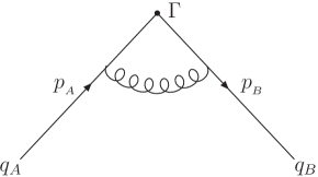
Figure 1: The one-loop vertex correction to the quark form factor.

A way to disentangle the scales is to substitute the full theory with simpler but equivalent effective theories by systematically integrating out the heavy degrees of freedom scale by scale. The basic idea of summing large logarithms in the effective theory had been explained in the Introduction. Now we use the SCET to separate the scales in the Sudakov form factor.

The hard region with virtual momenta of $k\sim Q(1,1,1)$ is the hard mode which contributes to the Wilson coefficient. An infinite collinear gluons couple to the hard loops and the collinear quark moves in another direction have momentum virtuality of $Q^{2}$ without suppression in leading order of $\lambda$. Because of gauge invariance, it is convenient to use the explicit gauge-invariant quantities. The collinear quark $\xi(x)$ transforms to $U_{c}(x)\xi(x)$ under the collinear gauge transformation. The collinear Wilson line transforms as $W_{c}(x)\to U_{c}(x)W_{c}(x)$. A gauge invariant combination of them is is a gauge singlet $W_{c}^{\dagger}\xi$ under collinear gauge transformations. This gauge singlet operator includes the interactions of collinear gluons with the hard loops and the collinear quark moves in another direction.

The couplings of soft gluons to the collinear filed lead to off-shellness of $Q^{2}\lambda\gg Q^{2}\lambda^{2}$. Integrating out this off-shell modes gives soft Wilson line $W_{s}$. After this, the soft gluons decouple from the collinear fields. Under the soft gauge transformations $U_{s}(x)$, the collinear fields is unchanged and the soft Wilson lines transforms as $W_{s}(n_{-})\to U_{s}W_{s}(n_{-})$, $W_{s}(n_{+})\to U_{s}W_{s}(n_{+})$ where $W_{s}(n)$ represents the collinear Wilson line along the $n$ direction. The combination of $W_{s}(n_{-})^{\dagger}W_{s}(n_{+})$ is invariant under the soft gauge transformations.

The above discussions give a gauge invariant expression for the current operator in SCET as

$$\bar{\xi}_{n_{-}}W_{c}(n_{+})W_{c}^{\dagger}(n_{-})\xi_{n_{+}}(\mu)W_{s}(n_{-})^{\dagger}W_{s}(n_{+}).$$ (9)

where $\xi_{n_{+}}$ and $W_{c}(n_{-})$ represent the collinear fields move along the $n_{-}$ direction. Similar interpretations for the other operators are implied. The effective operator includes all the low-energy dynamics but no high-energy dynamics. The hard mode with virtualities of $k\sim Q(1,1,1)$ needs to be included when we match the full theory onto the effective theory since the prediction of the two methods must be equal to a given order of $\lambda$. The matching of the current operator gives

$$V_{\Gamma}=\int dsds^{\prime}\tilde{C}(s,s^{\prime},\mu)\left[\bar{\xi}_{n_{-}}W_{c}(n_{+})\right](sn_{+})\Gamma\left[W_{c}(n_{-})\xi_{n_{+}}\right](s^{\prime}n_{-})W_{s}(n_{-})^{\dagger}W_{s}(n_{+}),$$ (10)

The $\tilde{C}(s,s^{\prime},\mu)$ is position space Wilson coefficient which depends on the position of the collinear field. The appearance of integral over $s$ is due to that the momenta $p_{A}^{+}$, $p_{B}^{-}$ are at order of $Q$.

The matrix element $\langle q_{B}|\bar{\psi}_{B}\gamma_{\mu}\psi_{A}|q_{A}\rangle$ then becomes

$$\langle q_{B}|\bar{\psi}_{B}\gamma_{\mu}\psi_{A}|q_{A}\rangle = \gamma_{\mu}\int dsds^{\prime}\tilde{C}(s,s^{\prime},\mu)\left\langle q_{B}\left|\left[\bar{\xi}_{n_{-}}W_{c}(n_{+})\right](sn_{+})\right|0\right\rangle$$ (11)

$$~{}~{}\times\left\langle 0\left|\left[W_{c}(n_{-})\xi_{n_{+}}\right](s^{\prime}n_{-})\right|q_{A}\right\rangle\langle 0|W_{s}(n_{-})^{\dagger}W_{s}(n_{+})|0\rangle$$

$$= C(n_{+}\cdot p_{B},n_{-}\cdot p_{A},\mu)\left\langle q_{B}\left|\left[\bar{\xi}_{n_{-}}W_{c}(n_{+})\right]\right|0\right\rangle$$

$$~{}~{}\times\left\langle 0\left|\left[W_{c}(n_{-})\xi_{n_{+}}\right]\right|q_{A}\right\rangle\langle 0|W_{s}(n_{-})^{\dagger}W_{s}(n_{+})|0\rangle$$

In the above equation, we have used the translation invariance $\phi(a)=e^{ia\cdot P}\phi(0)e^{-ia\cdot P}$. The $C(n_{+}\cdot p_{B},n_{-}\cdot p_{A},\mu)$ is the momentum space Wilson coefficient defined by

$$C(n_{+}\cdot p_{B},n_{-}\cdot p_{A},\mu)=\int dsds^{\prime}e^{isn_{+}\cdot p_{B}}e^{-isn_{-}\cdot p_{A}}~{}\tilde{C}(s,s^{\prime},\mu),$$ (12)

In SCET, there is remnant Lorentz invariance called by reparameterization invariance. One class is the longitudinal boosts $n_{+}\to\alpha n_{+}$, $n_{-}\to\alpha^{-1}n_{-}$. The Lorentz invariance constraints the $C(n_{+}\cdot p_{B},n_{-}\cdot p_{A},\mu)$ can only depend on $(n_{+}\cdot p_{B})(n_{-}\cdot p_{A})=Q^{2}$. The dimensionless hard Wilson coefficient make us to simplify $C(n_{+}\cdot p_{B},n_{-}\cdot p_{A},\mu)=C(Q/\mu)$.

Thus, we obtain a final explicit factorized form for the form factor $F(Q^{2})$ as

$$F(Q^{2})=C(\mu)~{}J_{A}~{}J_{B}~{}S.$$ (13)

where $J_{A}$, $J_{B}$ and $S$ are defined by

$$J_{A} \equiv \langle 0|{\rm P~{}exp}\left(ig_{s}\int_{0}^{+\infty}dt~{}n_{-}\cdot A_{c}(tn_{-})\right)\xi_{n_{+}}|q_{A}\rangle;$$

$$J_{B} \equiv \langle q_{B}|\bar{\xi}_{n_{-}}~{}{\rm P~{}exp}\left(ig_{s}\int_{-\infty}^{0}dt~{}n_{+}\cdot A_{c}(tn_{-})\right)|0\rangle;$$ (14)

$$S~{} \equiv \langle 0|{\rm P~{}exp}\left(ig_{s}\int_{0}^{+\infty}dt~{}n_{-}\cdot A_{s}(tn_{-})\right){\rm exp}\left(ig\int_{-\infty}^{0}dt~{}n_{+}\cdot A_{s}(tn_{+})\right)|0\rangle.$$

The above factorization formulae is consistent with the result given in Collins ; Korchemsky .

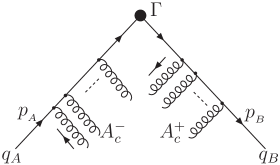
Figure 2: The collinear gluons contribute to the collinear Wilson lines. The $A_{c}^{+}$ and $A_{c}^{-}$ represent the gluons collinear to quarks $q_{A}$ and $q_{B}$ respectively.

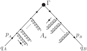
Figure 3: The soft gluons contribute to the soft Wilson lines.

Expanding the path-ordered exponential of Wislon line $W$ in orders of the coupling constant gives the Feynman rules in momentum space

$${\rm P~{}exp}\left(ig_{s}\int_{0}^{+\infty}dt~{}n\cdot A(tn)\right)=1+{\rm P}\sum\limits_{i=1}^{\infty}\prod\limits_{j=1}^{i}\int\frac{d^{4}k_{j}}{(2\pi)^{4}}ig_{s}n\cdot\tilde{A}(k_{j})\frac{i}{n\cdot\sum_{j=1}^{i}k_{j}}.$$ (15)

where $\tilde{A}(k_{j})$ are Fourier conjugated field of gluon $A(tn)$.

The soft and collinear Wilson lines are plotted in Fig. 2 and Fig. 3. The jet-A function is defined as a matrix element of the quark field $A$ with a path-ordered Wilson line which accumulates an infinite gluons collinear to A from point 0 (the hard scattering point) to $+\infty$ along the $n_{-}$ direction. The jet-B function is defined as a matrix element of the quark field $B$ with a path-ordered Wilson line which an infinite collinear-to-B gluons go from $-\infty$ to the point $0$ along the $n_{-}$ direction. The soft function $S$ is independent of the quark flavor and spin. This is due to an additional spin-flavor symmetry for the interactions of collinear quark with soft gluons in SCET. The $S$ is defined as the vacuum expectation value of soft Wilson lines. The soft gluons go from $-\infty$ to point 0 along the $n_{+}$ direction and then from point 0 to $+\infty$ along the $n_{-}$ direction. Note that the Wilson line is unitary, i.e., $W^{\dagger}W=1$. The path-ordering in the Wilson line is similar to the time-ordering in the conventional quantum field theory and the parameter $t$ acts as time.

II.3 The summation of Sudakov-logs in SCET

The calculation of the Wilson coefficient $C(\mu)$ is performed by a matching procedure from the full theory onto the effective theory. Because the origin of the Wilson coefficient $C(\mu)$ is insensitive to the detail of IR physics, one is free to choose any infrared regularization method and the external states. For the quark form factor, the most convenient way is to use the dimensional regularization method and to perform the matching on mass shell of the massless quark. In the dimensional regularization, all the loop corrections to the long-distance functions $J_{A}$, $J_{B}$ and $S$ vanish because there is no scale parameter in the loop integral. The only remained integral is coming from contribution of the hard part which the momentum of the virtual quark $k\sim Q(1,1,1)$. The one-loop contribution to the quark form factor in $d=4-2\epsilon$ dimension is

$$I = -ig_{s}^{2}C_{F}\mu^{\prime 2\epsilon}\int\frac{d^{d}k}{(2\pi)^{d}}\frac{\gamma_{\rho}(\hbox to0.0pt{\hskip 0.56917pt/\hss}{k}+\hbox to0.0pt{\hskip 0.56917pt/\hss}{p}_{B})\gamma_{\mu}(\hbox to0.0pt{\hskip 0.56917pt/\hss}{k}+\hbox to0.0pt{\hskip 0.56917pt/\hss}{p}_{A})\gamma^{\rho}}{[k^{2}+2p_{A}\cdot k+i\epsilon][k^{2}+2p_{B}\cdot k+i\epsilon][k^{2}+i\epsilon]}$$ (16)

$$= \frac{\alpha_{s}}{4\pi}C_{F}\gamma_{\mu}\left[-\frac{2}{\epsilon^{2}}-\frac{3+2{\rm ln}\frac{\mu^{2}}{Q^{2}}}{\epsilon}-{\rm ln}^{2}\frac{\mu^{2}}{Q^{2}}-3{\rm ln}\frac{\mu^{2}}{Q^{2}}-8+\frac{\pi^{2}}{6}\right].$$

where $\mu^{2}=4\pi\mu^{\prime 2}{\rm e}^{-\gamma_{E}}$ is the scale defined in the ${\rm\overline{MS}}$ scheme and $\gamma_{E}$ is the Euler constant.

The one-loop correction is divergent and requires renormalization. This is different from the result in the full theory. We need not care about whether the divergence is of UV or IR type in the dimensional regularization when doing renormalization, although the divergences are IR in origin. The renormalization in the effective field theory can be done by the standard counter-term method. The coefficient $C$ is regarded as coupling constant. One way to perform the renormalization is done by redefining the coefficient $C$ while leaving the operators in SCET unrenormalized as follows

$$C^{0}=Z_{C}C,~{}~{}~{}~{}~{}~{}~{}Z_{C}=1-\frac{\alpha_{s}}{4\pi}C_{F}\left[\frac{2}{\epsilon^{2}}+\frac{3+2{\rm ln}\frac{\mu^{2}}{Q^{2}}}{\epsilon}\right].$$ (17)

The $C^{0}$ represents the bare coupling constant. The renormalization constant $Z_{C}$ contains momentum $Q$-dependent counter-term which will contribute to a momentum-dependent anomalous dimension. There is a $\frac{1}{\epsilon^{2}}$ double-poles in one loop order of the $Z_{C}$. This is not familiar in the standard perturbation theory. The appearance of the double-poles is due to the overlap of soft and collinear divergences in the effective theory when the low energy scale approaches 0. The $Z_{C}$ does not depend on the low-energy scale. The renormalized matching coefficient $C(\mu)$ up to one-loop order is

$$C(\mu)=1+\frac{\alpha_{s}}{4\pi}C_{F}\left[-{\rm ln}^{2}\frac{\mu^{2}}{Q^{2}}-3{\rm ln}\frac{\mu^{2}}{Q^{2}}-8+\frac{\pi^{2}}{6}\right].$$ (18)

The renormalization in SCET can be done in a different but equivalent way. Another method is the conventional operator renormalization which renormalizes the operators rather than the coefficients. For this method, we need to know the exact UV divergences of the operators in SCET. We also provide this renormalization method for reference. From the results of Appendix, the renormalization constants for $J_{A}$, $J_{B}$ and $S$ are

$$Z_{A}:~{}~{}~{}~{}~{} \frac{\alpha_{s}}{4\pi}C_{F}\left[\frac{2}{\epsilon^{2}}+\frac{2+2{\rm ln}\frac{\mu^{2}}{Q\delta}}{\epsilon}+\frac{-1}{2\epsilon}\right],$$

$$Z_{B}:~{}~{}~{}~{}~{} \frac{\alpha_{s}}{4\pi}C_{F}\left[\frac{2}{\epsilon^{2}}+\frac{2+2{\rm ln}\frac{\mu^{2}}{Q\delta}}{\epsilon}+\frac{-1}{2\epsilon}\right],$$

$$Z_{S}:~{}~{}~{}~{}~{} \frac{\alpha_{s}}{4\pi}C_{F}\left[-\frac{2}{\epsilon^{2}}-\frac{2{\rm ln}\frac{\mu^{2}}{\delta^{2}}}{\epsilon}\right],$$

$$Total:~{}~{}~{} \frac{\alpha_{s}}{4\pi}C_{F}\left[\frac{2}{\epsilon^{2}}+\frac{3+2{\rm ln}\frac{\mu^{2}}{Q^{2}}}{\epsilon}\right],$$ (19)

where the $\frac{\alpha_{s}}{4\pi}C_{F}\frac{-1}{2\epsilon}$ terms for $J_{A}$ and $J_{B}$ are coming from the quark field $\xi$ renormalization. The total counter-term $Z_{T}$ can be obtained from Eq. (II.3) as

$$Z_{T}=\frac{\alpha_{s}}{4\pi}C_{F}\left[\frac{2}{\epsilon^{2}}+\frac{3+2{\rm ln}\frac{\mu^{2}}{Q^{2}}}{\epsilon}\right].$$ (20)

$Z_{T}$ is the negative of the relevant term of $Z_{C}$ in Eq. (17). There is a general relation of the renormalization constants in the operator renormalization and the coefficient renormalization: $Z_{T}=Z_{C}^{-1}$ Buras .

In Eq. (17), the bare coupling constant $C^{0}$ is $\mu$-independent. Using the relation $\mu\frac{dC^{0}}{d\mu}=0$, we obtain a renormalization group equation for $C(\mu)$ as

$$\mu\frac{d}{d\mu}C(\mu)=\left(\mu\frac{\partial}{\partial\mu}+\beta(g)\frac{\partial}{\partial g}\right)C(\mu)=\gamma_{C}C(\mu).$$ (21)

Here, the anomalous dimension $\gamma_{C}$ is defined by

$$\gamma_{C}=-\frac{1}{Z_{C}}~{}\frac{dZ_{C}}{d{\rm ln}\mu}=\frac{1}{Z_{T}}~{}\frac{dZ_{T}}{d{\rm ln}\mu},$$ (22)

The direct way to calculate the anomalous dimension is through the $1/\epsilon$-pole terms of the renormalization constant. From the result in Eq. (17), the anomalous dimension $\gamma_{C}$ is obtained up to $\alpha_{s}$ order as

$$\gamma_{C}=2\alpha_{s}\frac{\partial Z_{C,1}}{\partial\alpha_{s}}=-\frac{\alpha_{s}}{2\pi}C_{F}\left(3+2{\rm ln}\frac{\mu^{2}}{Q^{2}}\right).$$ (23)

where $Z_{C,1}$ is the $1/\epsilon$-pole coefficient of $Z_{C}$. Note that in the derivation of the above evolution equation we used the non-renormalization property for the collinear and soft fields. One property of the anomalous dimension $\gamma_{C}$ is its Q-dependence. Another thing is that the anomalous dimension in leading logarithmic approximation (here, the leading logarithmic approximation refers to the leading double-logarithmic approximation) is positive, i.e., $\gamma_{C}=\frac{\alpha_{s}}{\pi}C_{F}{\rm ln}\frac{Q^{2}}{\mu^{2}}>0$ for $\mu\ll Q$. That means $C(\mu)$ is a decreasing function as $Q$ increases or $\mu$ decreases. This provides an explanation of the suppression of the Sudakov form factor.

The solution of the renormalization group equation like Eq. (21) is an exponential form in general

$$C(\mu_{0}) = C(Q)~{}{\rm exp}\left[\int_{{\rm ln}Q}^{{\rm ln}\mu_{0}}d({\rm ln}\mu)\gamma_{C}(g(\mu))\right]$$ (24)

$$= C(Q)~{}{\rm exp}\left[\int_{g(Q)}^{g(\mu_{0})}dg\frac{\gamma_{C}(g)}{\beta(g)}\right].$$

For our case, the one-loop calculations give $C(Q)=1+\frac{\alpha_{s}}{4\pi}C_{F}\left[-8+\frac{\pi^{2}}{6}\right]$ and $\gamma_{C}=-\frac{\alpha_{s}}{2\pi}C_{F}\left(3+2{\rm ln}\frac{\mu^{2}}{Q^{2}}\right)$. The scale $\mu_{0}$ is a low energy scale but be chosen to guarantee the smallness of the coupling constant $\alpha_{s}$.

The solution of the renormalization group equation sums the series of large logarithms $\alpha_{s}^{n}{\rm ln}^{m}Q^{2}(m\leq 2n)$ to all orders automatically. We define the leading-log (LL) and next-to-leading-log (NLL) approximations for summation as

$${\rm LL~{}~{}}:~{}~{}~{}~{}~{} \sum\limits_{n}\alpha_{s}^{n}~{}({\rm ln}Q^{2})^{2n};$$

$${\rm NLL}:~{}~{}~{}~{}~{} \sum\limits_{n}\alpha_{s}^{n}~{}({\rm ln}Q^{2})^{2n-1}.$$ (25)

The LL and NLL approximations are valid if the relations below are satisfied

$$\alpha_{s}\ll\alpha_{s}{\rm ln}Q^{2}\ll\alpha_{s}{\rm ln}^{2}Q^{2}\sim{\cal O}(1).$$ (26)

At first sight, the coefficient $C(\mu_{0})$ has no relation with the Sudakov form factor. The meaning of the coefficient $C(\mu_{0})$ will be clear after we discuss a simple case of the solution of Eq. (21). In the LL approximation,

$$C(Q)=1,~{}~{}~{}~{}~{}~{}\gamma_{C}^{\rm LL}=-2\frac{\alpha_{s}}{\pi}C_{F}{\rm ln}\frac{\mu}{Q}.$$ (27)

We consider a case that the coupling constant $g_{s}$ is frozen at a finite value, or say the running effect is neglected. From Eq. (24), we obtain a solution for this simple case as

$$C(\mu_{0})={\rm exp}\left[-\frac{\alpha_{s}}{4\pi}C_{F}{\rm ln}^{2}\frac{Q^{2}}{\mu_{0}^{2}}\right].$$ (28)

This reminds us the familiar result $F={\rm exp}\left[-\frac{g^{2}}{16\pi^{2}}{\rm ln}^{2}\frac{Q^{2}}{m^{2}}\right]$ in QED when $C_{F}=1$ and $\mu_{0}=m$. We can say that: the Wilson coefficient $C(\mu_{0})$ is the perturbative part of the usual Sudakov form factor. When the quark confinement is ignored, $C(\mu_{0})$ is equal to $F(Q^{2})$. The exponentiation of the Sudakov form factor is explained by the solution of a renormalization group equation. The mechanism for the exponentiation of Sudakov form factor is the same as other physical quantities which satisfy the RG evolution equations.

The effect of the running of the coupling constant can be included straightforwardly by using $\alpha_{s}(\mu)=\frac{4\pi}{\beta_{0}~{}{\rm ln}(\mu^{2}/\Lambda^{2})}$ and $\beta(g)=-\beta_{0}g\frac{\alpha_{s}}{4\pi}$ in LL approximation. The solution of $C(\mu_{0})$ is

$$C(\mu_{0})={\rm exp}\left\{-4\frac{C_{F}}{\beta_{0}}\left[{\rm ln}\frac{Q}{\Lambda}{\rm ln}\frac{{\rm ln}Q/\Lambda}{{\rm ln}\mu_{0}/\Lambda}-{\rm ln}\frac{Q}{\mu_{0}}\right]\right\}.$$ (29)

or written in another form

$$C(\mu_{0})={\rm exp}\left\{\frac{8\pi C_{F}}{\beta_{0}^{2}\alpha_{s}(Q)}\left[1-\frac{1}{z}-{\rm ln}z\right]\right\}.$$ (30)

where $z=\frac{\alpha_{s}(\mu_{0})}{\alpha_{s}(Q)}$ is defined in B2 .

In NLL approximation, the anomalous dimension contains one-loop order as well as two-loops order corrections. We will not do an explicit two-loops calculation but use the results provided in KR ; Collins . In NLL, we the anomalous dimension is written as

$$\gamma_{C}^{\rm NLL}=-\frac{\alpha_{s}}{4\pi}C_{F}6-(\frac{\alpha_{s}}{\pi})^{2}C_{F}B~{}{\rm ln}\frac{\mu}{Q},$$ (31)

where the coefficient $B$ will be determined by other methods.

The momentum-dependent anomalous dimension has been calculated as a cusp dimension up to two-loops order as KR ; Collins

$$\Gamma=-\left\{2\frac{\alpha_{s}}{\pi}C_{F}+\left[\left(\frac{67}{18}-\frac{\pi^{2}}{6}\right)C_{A}-\frac{10}{9}n_{f}T_{F}\right]\left(\frac{\alpha_{s}}{\pi}\right)^{2}C_{F}\right\}{\rm ln}\frac{\mu}{Q},$$ (32)

where $n_{f}$ is the number of quark flavors and the SU(3)_C group constants are: $T_{F}=\frac{1}{2}$, $C_{F}=\frac{4}{3}$ and $C_{A}=3$.

From the comparison of Eqs.(27, 31) with Eq. (32), we obtain the coefficient $B$ as

$$B=\left(\frac{67}{18}-\frac{\pi^{2}}{6}\right)C_{A}-\frac{10}{9}n_{f}T_{F}.$$ (33)

In order to calculate the Sudakov form factor to NLL, we need the function $\beta(g)$ and coupling constant $\alpha_{s}$ to next-to-leading order Buras ,

$$\beta(g) = -\beta_{0}g\frac{\alpha_{s}}{4\pi}\left(1+\frac{\beta_{1}}{\beta_{0}}\frac{\alpha_{s}}{4\pi}\right),$$

$$\alpha_{s}(\mu) = \frac{4\pi}{\beta_{0}~{}{\rm ln}(\mu^{2}/\Lambda^{2})}\left(1-\frac{\beta_{1}}{\beta_{0}^{2}}\frac{{\rm ln}~{}{\rm ln}(\mu^{2}/\Lambda^{2})}{{\rm ln}(\mu^{2}/\Lambda^{2})}\right),$$

$${\rm ln}\frac{\mu}{Q} = \frac{2\pi}{\beta_{0}}\left[\frac{1}{\alpha_{s}(\mu)}-\frac{1}{\alpha_{s}(Q)}+\frac{\beta_{1}}{4\pi\beta_{0}}{\rm ln}\frac{\alpha_{s}(\mu)}{\alpha_{s}(Q)}\right].$$ (34)

where $\beta_{0}=\frac{(11N_{c}-2n_{f})}{3}$ and $\beta_{1}=\frac{34}{3}N_{c}^{2}-\frac{10}{3}N_{c}n_{f}-2C_{F}n_{f}$ with $N_{c}=3$.

The final formula for coefficient $C(\mu_{0})$ up to NLL approximation is

$$C(\mu_{0})=e^{S(Q,\mu_{0})}.$$ (35)

where we have taken approximation $C(Q)=1$. The factor $S(Q,\mu_{0})$ is

$$~{}S=S^{LL}+S^{NLL},~{}~{}~{}~{}~{}~{}~{}~{}~{}S^{LL}=\frac{8\pi C_{F}}{\beta_{0}^{2}\alpha_{s}(Q)}\left[1-\frac{1}{z}-{\rm ln}z\right],$$

$$S^{NLL}=\frac{3C_{F}}{\beta_{0}}{\rm ln}z+\frac{4C_{F}}{\beta_{0}^{2}}B(1-z+{\rm ln}z)+\frac{2C_{F}\beta_{1}}{\beta_{0}^{3}}(z-1-{\rm ln}z+\frac{1}{2}{\rm ln}^{2}z).$$ (36)

The term $S^{LL}(Q,\mu_{0})$ is the result of the LL approximation which had been given in Eq. (30). The NLL term $S^{NLL}(Q,\mu_{0})$ is suppressed by a logarithm ${\rm ln}Q^{2}$ compared to the leading factor $S^{LL}(Q,\mu_{0})$.

Figure 4: The Q-dependence of Sudakov form factor $e^{S(Q,\mu_{0})}$ including both the LL and NLL contributions. The variables Q are given in units of GeV.

The coefficient $C(\mu_{0})$, or say the Sudakov form factor $e^{S(Q,\mu_{0})}$ is a decreasing function of $Q$. Fig. 4 shows that Sudakov form factor $e^{S(Q,\mu_{0})}$ damps as $Q$ increases. The suppression of the Sudakov form factor is due to negative value of the LL factor $S^{LL}(Q,\mu_{0})$. However, the NLL factor $S^{NLL}(Q,\mu_{0})$ is positive and has a destructive effect on the suppression of the LL result. Fig. 5 plots the $Q$-dependence of factors $S^{LL}$ and $S^{NLL}$. In order to ensure the convergence of summation series, the NLL contribution should be much smaller than the leading one. We check this by using the ratio $-S^{NLL}/S^{LL}$. From Fig. 6, the ratio $-S^{NLL}/S^{LL}$ becomes much smaller than 1 when $Q$ is very large. The parameters are chosen as: the QCD scale $\Lambda=0.25{\rm GeV}$; the quark flavor number $n_{f}=4$ and the scale $\mu_{0}=1.0{\rm GeV}$.

Figure 5: The Q-dependence of factors $S^{LL}$ and $S^{NLL}$. The upper curve is plotted for $S^{NLL}$ and the lower one for $S^{LL}$.

Figure 6: The ratio of $-S^{NLL}/S^{LL}$ vs energy scale $Q$.

II.4 The interpretation of $F(Q^{2})$

In the discussions below, we will neglect the confinement effect and set $C(\mu_{0})=F(Q^{2})$. Because the Sudakov form factor is a dimensionless quantity, the naive expectation from tree level consideration is that it is a constant: $F=1$. The radiative corrections change it to dependent on energy $F(Q^{2})=F(Q^{2}/m^{2})$. Because the radiative corrections is perturbative, one may expect that the deviation of $F(Q^{2})$ from $1$ is of order of $\alpha_{s}$ and thus small. The result from resummation tells us that the naive thinking is wrong. The $F(Q^{2})$ damps fast to zero when $Q$ is large enough. One explanation of this non-trivial result is that the large logarithms modify the perturbative series and the sum of them to all orders is the correct result. Here, we give another explanation from scale point of view: the Sudakov form factor is a multi-scales system, the intermediate scales are all important and the sum of contributions from all scales gives the Sudakov form factor.

The scales in the Sudakov form factor are $Q,~{}m$ and the intermediate scales between them. The crucial feature for the intermediate region is the absence of characteristic energy scales. Because of this feature, we can apply the Wilson’s renormalization group method WilsonRG . The principle (or say assumption) behind this method is that the many energy scales are locally coupled. The dynamics associated with each energy scale can be interpreted as a superposition in scale space. It means: the high momentum fluctuations at $Q$ does not couple importantly to the low momentum fluctuations at $m$, the coupling of momentum fluctuations at scale $\mu$ to the fluctuations at scale $\mu/10$ is weaker than to scale $\mu/2$. The result of the local property is a cascade mechanism: the fluctuation of $Q$ influences fluctuation of $Q/2$; the fluctuation of $Q/2$ influences fluctuation of $Q/4$; etc. until to the low momentum fluctuations of $m$. The treatment of multi-scales problem can be done by integrating out the fluctuations scale by scale: first integrate out fluctuation of $Q$ and obtain $C(Q)$, then integrate out fluctuations between $Q$ and $Q/2$ and obtain $C(Q)$; etc. at the end we obtain $C(m)=F(Q^{2})$. The cascade chain can also be performed continuously from $\mu\to\mu-d\mu$. This gives the evolution equation of Eq. (21). The solution of the evolution equation from high to low energy scales gives the Sudakov form factor.

In SCET, the cascade mechanism is realized as: First, we integrate out the momentum fluctuations at scale $\mu=Q$ and obtain an effective current $V_{QCD}=C(Q)V_{SCET}(Q)$; Second, we integrate out the intermediate scales step by step to the low energy which corresponds to solve the evolution equation of Eq. (21); At last we obtain $V_{QCD}=C(m)V_{SCET}(m)$, the Sudakov form factor is included in $C(m)$.

Because there is no characteristic scale in the intermediate regions, the similar effects should occur for each step of the cascade chain. It leads to one feature of the cascade mechanism: the existence of amplification or deamplification as cascade develops. Whether the effect is amplification or deamplification depends on the sign of dimension function in the evolution equation. In other words, if the influence of fluctuations of scale $\mu$ on fluctuations of $\mu-d\mu$ is negative, the deamplification occurs. The Sudakov form factor belongs to the deamplification effect. The larger space for the cascade developing when $Q$ increases, the higher the suppression is. As have been discussed, it is the cusp dimension dimension that determines the suppression of the Sudakov form factor.

The above picture illustrates the idea behind the effective field theory. It explains why the factorization in SCET are different from the diagrammatic analysis. For the technical calculations, the dimensional regularization method and the conventional renormalization procedure are convenient and useful in perturbation theory. Note that the application of the effective field theory does not restricted in the perturbation theory, one example is the chiral perturbation theory.

III Comparison with other methods of Sudakov resummation

In the last section, we have discussed the Sudakov resummation in the soft-collinear effective theory by utilizing the renormalization group method. The Sudakov form factor had been got extensive studies in the literatures. Here, we want to compare our approach with other methods. However, the approaches about Sudakov resummation appeared in literatures are too much to be considered fully. We choose three methods for discussion: the leading double-logarithmic approximation method, the Wilson loop method and the CSS method. We will not concern the technical details but the main concepts.

III.1 The leading double-logarithmic approximation method

The explicit calculation of the Sudakov form factor order by order is instructive to understand the relation between the RG method and the Feynman diagram method. The calculation of the Sudakov form factor beyond the $\alpha_{s}$ order in QCD is complicate due to the self-interactions of gluon fields CPQ . We will discuss the case of QED at first to obtain some insights. In Feynman gauge, the leading contributions (in leading double-logarithmic approximation) to the vertex correction come from the ladder and crossed-ladder graphs which is plotted in Fig. 7. About the method of the leading double-logarithmic approximation, we refer to recent papers of FLMM ; ET .

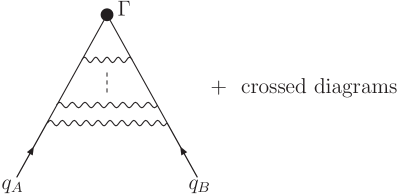
Figure 7: The ladder graphs of quark form factor in QED in the leading double-logarithmic approximation.

The mechanism for appearance of the double-logarithms is: an energetic quark emits a soft and quasi-collinear photon and then the photon is absorbed by another collinear quark. If the quark emits a pure collinear or soft photon, there is only single logarithm. When the soft and collinear regions overlap, the double-logarithms appear. The extension of the leading order mechanism to all orders can be pictured as a cascade chain $qq\to qq\to qq\to...$ by infrared photon exchange which contributes to the ladder graphs in QED. The quark scattering satisfies a local property that the quark scattering of a given level does not depend on the details of the scattering at a deeper level. The simplest way to express the cascade chain is through an infrared evolution equation

$$F(\frac{Q^{2}}{\mu^{2}})=1-\int_{\mu^{2}}^{Q^{2}}\frac{\alpha(k_{\bot})}{2\pi}\frac{dk_{\bot}^{2}}{k_{\bot}^{2}}~{}{\rm ln}\frac{Q^{2}}{k_{\bot}^{2}}F(\frac{Q^{2}}{k_{\bot}^{2}}).$$ (37)

where $\mu$ is an infrared cut-off.

Differentiates Eq. (37) with $\mu$, we obtain

$$\frac{d}{d{\rm ln}\mu}F(\frac{Q^{2}}{\mu^{2}})=-\frac{\alpha}{\pi}{\rm ln}\frac{\mu^{2}}{Q^{2}}F(\frac{Q^{2}}{\mu^{2}})$$ (38)

The above equation coincides with the RG equation (21) with the LL anomalous dimension but the physical meaning is different. Our derivation starts from the hard function $C(\mu)$ with hard gluons exchange, the above infrared evolution equation considers the soft gluons exchange.

In the leading double-logarithmic approximation method, we find a cascade mechanism for Feynman diagrams, the locality of the cascade scattering and the related evolution equation. These ideas are analogous to our intuitive understanding about the renormalization group method although they are expressed in different languages.

At last, we discuss the dependence of the Sudakov form factor on the regularization methods. In Sudakov , the one-loop correction to the form factor is $-\frac{\alpha}{2\pi}{\rm ln}^{2}\frac{Q^{2}}{p^{2}}$ by using an off-shell regularization method where $p^{2}$ is the off-shellness of quarks. The photon mass regularization gives the one-loop correction as $-\frac{\alpha}{4\pi}{\rm ln}^{2}\frac{Q^{2}}{m_{\gamma}^{2}}$ where $m_{\gamma}$ is the fictitious mass of photon Jackiw . In our method of regularization, the one-loop result is $-\frac{\alpha}{8\pi}{\rm ln}^{2}\frac{Q^{2}}{\delta^{2}}$ . Different methods give results by a factor of $2$ or $4$ difference.

III.2 The Wilson loop method

Both the Wilson loop method and the CSS method in the next subsection utilize the RG technic to sum the double logarithms. The derivations of the evolution equations are done in a different way. We denote the approach which uses the cusp dimension explicitly as the Wilson loop method.

The main ingredient in the Wilson loop method is a a renormalization group equation for a gauge invariant renormalized soft function $W_{R}$:

$$\left(\mu\frac{\partial}{\partial\mu}+\beta(g)\frac{\partial}{\partial g}+\Gamma_{cusp}(\gamma,g)\right)W_{R}=0.$$ (39)

The derivation of the above equation uses the renormalization methods given in Polyakov ; BNS ; BGSN ; KR . In Polyakov , it is pointed out that the vacuum average of a Wilson loop with a cusp contains extra UV divergences even after the ordinary field renormalization. One advantage of the cusp dimension is that it involves more geometrical meanings.

The on-shell Sudakov form factor is discussed in Korchemsky . The author uses the methods in KR3 to give a factorized form which shares some similarities with our operator language. For example, the coupling of collinear gluons to the hard part vanishes in the axial gauge, their effects can be included by a gauge transformation in a general gauge. The final result is similar to our collinear gauge invariant quantity $W_{c}^{\dagger}\xi$. A renormalization group equation for hard function $F_{H}$ is derived by using the Eq. (39) as

$$\left(\mu\frac{\partial}{\partial\mu}+\beta(g)\frac{\partial}{\partial g}\right)\frac{dF_{H}(Q^{2}/\mu^{2})}{d{\rm ln}Q^{2}}=\Gamma_{cusp}(g)F_{H}(Q^{2}/\mu^{2}).$$ (40)

It is consistent with Eq. (21).

In Korchemsky2 , the off-shell Sudakov form factor is discussed. There are three scales for the off-shell case: $Q$, $M$ and $M^{2}/Q$ where $M^{2}=-p^{2}$. Our discussion for the on-shell case needs to be modified and one RG equation is insufficient. For the off-shell Sudakov form factor in SCET, we need two-step matching: the first step integrates out the hard mode with momentum fluctuations of $Q$, the next step integrates out the collinear mode with momentum fluctuations of $M$. The details about the two-step matching was discussed in radiative B decays BHLN .

III.3 The CSS method

We denote the approach given in CS ; CSS2 ; BottsS ; Collins as the CSS method. This method is based on the factorization theorem of pQCD. The intuitive picture behind the factorization is a reduced graph. The highly off-shell lines with four momenta of order of $Q$ are contracted to points. The reduced graph is constructed by pinch singular points and it represents a classical scattering process. In leading power of $1/Q$, the reduced graphs for the quark form factor contain collinear, soft and hard graphs. In SCET, the highly off-shell contributions are denoted as the heavy mode and they need to be integrated out to obtain a low energy effective theory. Because the two methods describe the same physics, the low energy physics in the SCET should be exactly equal to the contributions in the reduced graphs. The method of momentum regions BS extends the reduced graph analysis beyond leading power. The reduced graph analysis and the method of regions can be used to check that the SCET reproduces the IR physics of QCD. About the comparison of the factorizaiton between the CSS method and SCET, some discussions are given in B3 .

After separating the quark form factor into collinear, soft and hard parts, the CSS method differentiates the form factor $F$ with respect to ${\rm ln}Q$ and obtain functions $K$ and $G$ which do not contain double-logarithms

$$\frac{\partial{\rm ln}F}{\partial{\rm ln}Q}=K(m/\mu,g)+G(Q/\mu,g).$$ (41)

The functions $K,G$ are derived from a gauge dependence of the jet functions. The RG equations for the CSS method are

$$\mu\frac{dG}{d\mu}=-\mu\frac{dK}{d\mu}=\gamma_{K}.$$ (42)

For massless case in QCD, the $K$, $G$ and $\gamma_{K}$ are Collins

$$K = \frac{\alpha_{s}}{\pi}C_{F}\frac{1}{\epsilon};~{}~{}~{}~{}~{}~{}~{}~{}~{}G=-\frac{\alpha_{s}}{\pi}C_{F}\left[{\rm ln}\frac{Q^{2}}{\mu^{2}}-\frac{3}{2}\right];$$

$$\gamma_{K} = 2\frac{\alpha_{s}}{\pi}C_{F}+\left[\left(\frac{67}{18}-\frac{\pi^{2}}{6}\right)C_{A}-\frac{10}{9}n_{f}T_{F}\right]\left(\frac{\alpha_{s}}{\pi}\right)^{2}C_{F}.$$ (43)

Compared with the results of the last section in SCET, it is easy to obtain the relations below

$$G=-\gamma_{C},~{}~{}~{}~{}~{}~{}~{}~{}~{}~{}~{}~{}~{}~{}~{}~{}\Gamma=\gamma_{K}~{}{\rm ln}\frac{Q}{\mu}.$$ (44)

The interpretation of the function $G$ as the anomalous dimension $\gamma_{C}$ is not accidental because the $G$ function in the CSS method represents the short-distance contribution.

The position space representation of the CSS method had been applied into the inclusive processes in CS ; CSS2 , exclusive processes in BottsS ; LS and recently into the exclusive B meson decays in pQCD . Because the energy $Q$ is not large enough to ensure the condition $Q\gg 1/b\gg\Lambda_{\rm QCD}$, the consistency of applying the perturbative Sudakov form factor is problematic at the experimental accessible energy regions. This question was addressed in DSWY .

A worldline approach to the Sudakov form factor starts a view closer to the string theory is discussed in GKKS . This approach is applied into the pion form factor in SSK .

IV Discussions and conclusions

In this study, we have studied in detail the Sudakov form factor in the framework of soft-collinear effective field theory. In the effective theory, the Sudakov form factor is the coefficient function running from high to low scale. The exponentiation of the Sudakov form factor is due to that it is the solution of a renormalization group equation. To this extent, the renormalization group equation for the Sudakov form factor is similar to the evolution equations for the parton distribution functions in deep inelastic scattering and the evolution equation for the hadron distribution amplitude. The positive leading-logarithmic anomalous dimension lead to the suppression of the Sudakov form factor at large $Q$. We discuss an intuitive picture of the cascade mechanism behind the renormalization group method.

We compared our method with other approaches for the Sudakov resummation. The ladder diagrams in the double-logarithmic approximation method provides an analogy with the intuitive understanding of the renormalization group method. The Wilson loop method uses a cusp anomalous dimension which has a clear geometrical origin. The CSS method gives a factorization of the Sudakov form factor from diagrammatic analysis and uses two functions to define the renormalization group evolution. All the methods give the consistent results. This may indicate that our physical world can be interpreted from different and complementary points of view. As a personal opinion, we think that the method of integrating out energy scales step by step from the effective field theory is more natural and simpler for the multi-scales problem.

$Note~{}added:$ After the finish of the paper, we are informed that a factorization proof of the Sudakov form factor in SCET was discussed in B4 . The main difference is that they use the hybrid position-momentum representation while we will use the position space formulation.

Appendix A

In this appendix, we provide a detailed calculation of the one-loop corrections to the quark form factor. We use the regularization method proposed in BDS .

The one-loop vertex correction in the full theory is

$$I_{full} = -ig_{s}^{2}C_{F}\mu^{\prime 2\epsilon}\int\frac{d^{d}k}{(2\pi)^{d}}\frac{\gamma_{\rho}(\hbox to0.0pt{\hskip 0.56917pt/\hss}{k}+\hbox to0.0pt{\hskip 0.56917pt/\hss}{p}_{B})\gamma_{\mu}(\hbox to0.0pt{\hskip 0.56917pt/\hss}{k}+\hbox to0.0pt{\hskip 0.56917pt/\hss}{p}_{A})\gamma^{\rho}}{[(k+p_{A})^{2}+i\epsilon][(k+p_{B})^{2}+i\epsilon][k^{2}-\delta(n_{+}+n_{-})\cdot k+i\epsilon]}$$ (45)

$$= \frac{\alpha_{s}}{4\pi}C_{F}\gamma_{\mu}\int_{0}^{1}dx\int_{0}^{1-x}dy\left\{\Gamma(\epsilon)\left(\frac{4\pi\mu^{\prime 2}}{\Delta}\right)^{\epsilon}2(1-\epsilon)^{2}-\frac{2(1-x)(1-y)Q^{2}}{\Delta}\right\}$$

$$= \frac{\alpha_{s}}{4\pi}C_{F}\gamma_{\mu}\left[\frac{1}{\epsilon}+{\rm ln}\frac{\mu^{2}}{Q^{2}}-\frac{1}{2}{\rm ln}^{2}\frac{Q^{2}}{\delta^{2}}+2{\rm ln}\frac{Q^{2}}{\delta^{2}}-\frac{\pi^{2}}{3}\right]$$

where $\Delta=xyQ^{2}-(x+y)(1-x-y)Q\delta+(1-x-y)^{2}\delta^{2}$.

The collinear-to-A contribution is

$$J_{A} = -ig_{s}^{2}C_{F}\mu^{\prime 2\epsilon}\int\frac{d^{d}k}{(2\pi)^{d}}\frac{-\gamma_{\mu}2(p_{A}^{+}-k^{+})}{[k^{2}-2p_{A}\cdot k+i\epsilon]~{}(n_{-}\cdot k)~{}[k^{2}-\delta(n_{-}\cdot k)+i\epsilon]}$$ (46)

$$= -\frac{g_{s}^{2}}{2\pi}C_{F}\mu^{\prime 2\epsilon}\gamma_{\mu}\int_{0}^{Q}\frac{dk^{+}}{k^{+}}(p_{A}^{+}-k^{+})\int\frac{d^{d-2}k_{\bot}}{(2\pi)^{d-2}}\frac{1}{k_{\bot}^{2}+\delta k^{+}(1-\frac{k^{+}}{p_{A}^{+}})}$$

$$= \frac{\alpha_{s}}{4\pi}C_{F}\gamma_{\mu}\left[\frac{2}{\epsilon^{2}}+\frac{2+2{\rm ln}\frac{\mu^{2}}{Q\delta}}{\epsilon}+{\rm ln}^{2}\frac{\mu^{2}}{Q\delta}+2{\rm ln}\frac{\mu^{2}}{Q\delta}+4-\frac{\pi^{2}}{6}\right]$$

From the first to the second line of the above equation, we perform the $k^{-}$ integral first by closing the contour in the lower half plane. The $k^{-}$ pole is chosen as $k^{-}=\frac{k_{\bot}^{2}+\delta k^{+}-i\epsilon}{k^{+}}$ and the range $k^{+}$ is $0<k^{+}<p_{A}^{+}$. The divergence of $k_{\bot}\to\infty$ is regulated by choosing dimension $d<4$. There is another singularity coming from the momentum region $k^{+}\to 0$. The overlapping of the two singularities lead to the double poles $\frac{1}{\epsilon^{2}}$. The result of the collinear-to-B contribution $J_{B}$ is the same as $J_{A}$.

The soft contribution is

$$S = -ig_{s}^{2}C_{F}\mu^{\prime 2\epsilon}\int\frac{d^{d}k}{(2\pi)^{d}}\frac{2\gamma_{\mu}}{[n_{-}\cdot k+i\epsilon][n_{+}\cdot k+i\epsilon][k^{2}-\delta(n_{+}+n_{-})\cdot k+i\epsilon]}$$ (47)

$$= -\frac{g_{s}^{2}}{2\pi}C_{F}\mu^{\prime 2\epsilon}\gamma_{\mu}\int_{\delta}^{\infty}\frac{dk^{+}}{k^{+}}\int\frac{d^{d-2}k_{\bot}}{(2\pi)^{d-2}}\frac{1}{k_{\bot}^{2}+\delta k^{+}}$$

$$= \frac{\alpha_{s}}{4\pi}C_{F}\gamma_{\mu}\left[-\frac{2}{\epsilon^{2}}-\frac{2{\rm ln}\frac{\mu^{2}}{\delta^{2}}}{\epsilon}-{\rm ln}^{2}\frac{\mu^{2}}{\delta^{2}}-\frac{\pi^{2}}{6}\right]$$

The contour of the $k^{-}$ integral is closed in the lower half plane and choose the pole at $k^{-}=\frac{k_{\bot}^{2}+\delta k^{+}-i\epsilon}{k^{+}-\delta}$ with $k^{+}>\delta$. The soft function is Q-independent.

References

- (1) V. Sudakov, Zh. Eksp. Teor. Fiz. 30, 87 (1956); Sov. Phys. JETP. 3, 65 (1956).
- (2) J.M. Cornwall and G. Tiktopoulos, Phys. Rev. Lett. 35, 338 (1975), and Phys. Rev. D13, 3370 (1976); A.H. Mueller, Phys. Rev. D20, 2037 (1979); A. Sen, Phys. Rev. D24, 3281 (1981).
- (3) J.J. Carazzone, E.C. Poggio and H.R. Quinn, Phys. Rev. D11, 2286 (1975).
- (4) J.C. Collins, in , ed. A.H. Mueller (World Scientific, Singapore, 1989), p573-614, or arXiv: hep-ph/0312336.
- (5) G.P. Korchemsky, Phys. Lett. B 217, 330 (1989).
- (6) G.P. Korchemsky, Phys. Lett. B 220 629 (1989).
- (7) H. Contopanagos, E. Laenen and G. Sterman, Nucl. Phys. B 484 303-330 (1997).
- (8) C.W. Bauer, S. Fleming and M.E. Luke, Phys. Rev. D63, 014006 (2001).
- (9) C.W. Bauer, S. Fleming, D. Pirjol and I.W. Stewart, Phys. Rev. D63, 114020 (2001).
- (10) M.J. Dugan and B. Grinstein, Phys. Lett. B 255, 583 (1991).
- (11) S. Descotes-Genon and C.T. Sachrajda, Nucl. Phys. B 650, 356-390 2003.
- (12) S.W. Bosch, R.J. Hill, B.O. Lange and M. Neubert, Phys. Rev. D67, 094014 (2003).
- (13) A.J. Buras, arXiv: hep-ph/9806471.
- (14) G.P. Korchemsky and A.V. Radyushkin, Nucl. Phys. B 283, 342 (1987).
- (15) A.M. Polyakov, Nucl. Phys. B 164, 171 (1980).
- (16) G.P. Korchemsky and A.V. Radyushkin, Phys. Lett. B 279, 359-366 (1992).
- (17) J.C. Collins, D.E. Soper and G. Sterman, in , ed. A.H. Mueller (World Scientific, Singapore, 1989), p1-91.
- (18) C.W Bauer, D. Pirjol and I.W. Stewart, Phys. Rev. D65, 054022 (2002).
- (19) K.G. Wilson, Phys. Rept. 12, 75-200 (1974); Rev. Mod. Phys. 55, 583-600 (1983).
- (20) G. Sterman, arXiv: hep-ph/9508358.
- (21) K.G. Wilson, Phys. Rev. D10, 2445 (1974).
- (22) M. Beneke, A.P. Chapovsky, M. Diehl and T. Feldmann, Nucl. Phys. B 643, 431 (2002).
- (23) Z. Wei, Phys. Lett. B 586, 282-290 (2004).
- (24) C.W. Bauer, M.P. Dorsten and M. P. Salem, arXiv: hep-ph/0312302.
- (25) B.I. Ermolaev and S.I. Troyan, Nucl. Phys. B 590, 521-536 (2000).
- (26) V.S. Fadin, L.N. Lipatov, A.D. Martin and M. Melles, Phys. Rev. D61, 094002 (2000).
- (27) R. Jackiw, Ann. Phys. (N.Y.) 48, 292 (1968).
- (28) R.A. Brandt, F. Neri and M.-A. Sato, Phys. Rev. D24, 879 (1981).
- (29) R.A. Brandt, A. Gocksch, M.-A. Sato and F. Neri, Phys. Rev. D26, 3611 (1982).
- (30) G.P. Korchemsky and A.V. Radyushkin, Sov.J.Nucl.Phys. 45, 910 (1987), Yad.Fiz. 45, 1466-1478 (1987).
- (31) J.C. Collins and D.E. Soper, Nucl. Phys. B 193, 381-443 (1981).
- (32) J.C. Collins, D.E. Soper and G. Sterman, Nucl. Phys. B 250, 199-224 (1985).
- (33) J. Botts and G. Sterman, Nucl. Phys. B 325, 62-100 (1989).
- (34) M. Beneke and V.A. Smirnov, Nucl. Phys. B 522, 321 (1998).
- (35) H. Li and G. Sterman, Nucl. Phys. B 381, 129-140 (1992).
- (36) H. Li and H. Yu, Phys. Rev. Lett. 74, 4388-4391 (1995); Y. Keum, H. Li and A.I. Sanda, Phys. Lett. B 504, 6 (2001); C. Lü, K. Ukai and M. Yang, Phys. Rev. D63, 074009 (2001); D. Du, C. Huang, Z. Wei and M. Yang, Phys. Lett. B 520, 50-58 (2001), Erratum-ibid.B 530, 258 (2002); Z. Wei and M. Yang, Nucl. Phys. B 642, 263-289 (2002).
- (37) S. Descotes and C.T. Sachrajda, Nucl. Phys. B 625, 239-278 (2002); Z. Wei and M. Yang, Phys. Rev. D67, 094013 (2003).
- (38) G.C. Gellas, A.I. Karanikas, C.N. Ktorides and N.G. Stefanis, Phys. Lett. B 412, 95-103 (1997).
- (39) N.G. Stefanis, W. Schroers and H.-. Kim, Phys. Lett. B 449, 299-305 (1999).
- (40) C.W. Bauer, S. Fleming, D. Pirjol, I.Z. Rothstein and I.W. Stewart, Phys. Rev. D66, 014017 (2002).