TUM-HEP-545/04

MPP-2004-28

Prospects of accelerator and reactor neutrino
oscillation experiments for the coming ten years

P. Huber,  M. Lindner,  M. Rolinec,
T. Schwetz, and  W. Winter

^,,,,Physik–Department, Technische Universität München,

James–Franck–Strasse, D–85748 Garching, Germany

Max-Planck-Institut für Physik, Postfach 401212, D–80805 München, Germany

We analyze the physics potential of long baseline neutrino oscillation experiments planned for the coming ten years, where the main focus is the sensitivity limit to the small mixing angle $\theta_{13}$. The discussed experiments include the conventional beam experiments MINOS, ICARUS, and OPERA, which are under construction, the planned superbeam experiments J-PARC to Super-Kamiokande and NuMI off-axis, as well as new reactor experiments with near and far detectors, represented by the Double-Chooz project. We perform a complete numerical simulation including systematics, correlations, and degeneracies on an equal footing for all experiments using the GLoBES software. After discussing the improvement of our knowledge on the atmospheric parameters $\theta_{23}$ and $\Delta m^{2}_{31}$ by these experiments, we investigate the potential to determine $\theta_{13}$ within the next ten years in detail. Furthermore, we show that under optimistic assumptions and for $\theta_{13}$ close to the current bound, even the next generation of experiments might provide some information on the Dirac CP phase and the type of the neutrino mass hierarchy.

1 Introduction

Within the last ten years a huge progress has been achieved in neutrino oscillation physics. In particular, the results of the atmospheric neutrino experiments [1, 2, 3] and the K2K accelerator neutrino experiment [4] have demonstrated that atmospheric muon neutrinos oscillate predominately into tau neutrinos with a mixing angle close to maximal mixing. Furthermore, solar neutrino experiments [5, 6] and the KamLAND reactor neutrino experiment [7] have established that the reduced flux of solar electron neutrinos is consistently understood by the so-called LMA-MSW solution [8]. Looking back at these exciting developments, it is tempting to extrapolate where we could stand in ten years from now with the experiments being under construction or planned. Certainly, neutrino physics will turn from the discovery era to the precision age, which however, will make this field by no means less exciting. The next major challenge will be the determination of the third, unknown mixing angle $\theta_{13}$, which at present is only known to be small [9, 10]. Further important issues will be the determination of the neutrino mass hierarchy and, if $\theta_{13}$ turns out to be large enough, the Dirac CP phase. Three different classes of experiments are under discussion for the next generation of long-baseline oscillation experiments, which are able to address at least some of these topics: Conventional beam experiments, first-generation superbeams, and new reactor experiments with near and far detectors. In this study, we consider specific proposals for such experiments, which are under construction or in active preparation, and could deliver physics results within the next ten years.

An already existing conventional beam experiment is the K2K experiment [4], which is sending a neutrino beam from the KEK accelerator to the Super-Kamiokande detector. This experiment has already confirmed the disappearance of $\nu_{\mu}$ as predicted by atmospheric neutrino data, and with more statistics it will slightly reduce the allowed range of the atmospheric mass splitting $\Delta m_{31}^{2}$. In this study, we consider in detail the next generation of such conventional beam experiments, which are the MINOS experiment [11] in US, and the CERN to Gran Sasso (CNGS) experiments ICARUS [12] and OPERA [13]. These experiments are currently under construction and should easily obtain physics results within the next ten years, including five years of data taking.

Moreover, we consider the subsequent generation of beam experiments, the so-called superbeam experiments. They use the same technology as conventional beams with several improvements. The most advanced superbeam proposals are the J-PARC to Super-Kamiokande experiment (JPARC-SK) [14] in Japan, and the NuMI off-axis experiment [15], using a neutrino beam produced at Fermilab in US. For these two experiments specific Letters of Intent exist and we use the setups discussed in there. JPARC-SK and NuMI could deliver important new results towards the end of the timescale considered in this work.

Recently, there has been a lot of activity to investigate the potential of new reactor neutrino experiments [16]. It has been realized that the performance of previous experiments, such as CHOOZ [9, 10] or Palo Verde [17], can be significantly improved if a near detector is used to control systematics and if the statistics is increased [18, 19, 20]. A number of possible sites are discussed, including reactors in Brasil, China, France, Japan, Russia, Taiwan, and the US (see Ref. [16] for an extensive review). Among the discussed options are the KASKA project in Japan [19] at the Kashiwazaki-Kariwa power plant, several power plants in USA [21, 22] (e.g., Diablo Canyon in California or Braidwood in Illinois), and the Double-Chooz project [23] (D-Chooz), which is planned at the original CHOOZ site [10] in France.

The particular selection of experiments considered in this study is determined by the requirement that results should be available within about ten years from now. This either requires that the experiments are already under construction (such as MINOS, ICARUS, and OPERA), or that specific proposals (Letters of Intent) including feasibility studies exist. From the current perspective, the only superbeam experiments fulfilling this requirement are the JPARC-SK and NuMI projects. Concerning reactors, we consider in this study the Double-Chooz project [23], since this proposal has the advantage that a lot of infrastructure from the first CHOOZ experiment can be re-used. In particular, the existence of the detector hall drastically reduces the required amount of civil engineering, which is considered to be time-critical for a future reactor experiment. Therefore, it seems rather likely that a medium size experiment can be built at the CHOOZ site within a few years and deliver physics results during the timescale considered here. We would like to stress that other reactor experiments of similar size, such as the KASKA project in Japan [19], would lead to results similar to Double-Chooz. To fully explore the potential of neutrino oscillation experiments at nuclear reactors, we furthermore consider an even larger reactor neutrino experiment (Reactor-II). This could be especially interesting if a large value of $\theta_{13}$ was found. Reactor-II is the only exception for which we use an abstract setup, which could, in principle, be built at one of the sites mentioned above. For example, some projects discussed in the US, such as Diablo Canyon or Braidwood [22, 24], are similar to our Reactor-II setup. Such an experiment could be feasible within a timescale similar to the superbeam experiments, and could provide results at the end of the period considered in this work. Note that in this study, we do not consider oscillation experiments using a natural neutrino source, such as solar, atmospheric, or supernova neutrinos.

The outline of the paper is as follows: After a brief description of the considered experiments in Section 2, we discuss the analysis methods and some analytical qualitative features of our results in Section 3. The main results of this study are given in Sections 4, 5, 6, and 7. First, in Section 4, we investigate the improvement of the atmospheric parameters $\theta_{23}$ and $\Delta m_{31}^{2}$ from long-baseline experiments within ten years. Then we move to the discussion of the $\sin^{2}2\theta_{13}$ sensitivity limit if no finite value of $\sin^{2}2\theta_{13}$ can be established. We consider in Section 5 the conventional beam experiments MINOS, ICARUS, and OPERA. In Section 6, we discuss the potential of reactor neutrino experiments to constrain $\sin^{2}2\theta_{13}$, and we compare the final $\sin^{2}2\theta_{13}$ bounds from the conventional beams, Double-Chooz, JPARC-SK, and NuMI. In Section 7, we investigate the assumption that $\sin^{2}2\theta_{13}$ is large, and discuss what we could learn from the next generation of experiments on the Dirac CP phase and the type of the neutrino mass hierarchy. In this section, the Reactor-II setup will become important. A summary of our results is given in Section 8. In Appendix A, we describe in detail our simulation of MINOS, ICARUS, and OPERA. Furthermore, in Appendix B, technical details of the reactor experiment analysis are given. Eventually, we present a thorough discussion of our definition of the $\sin^{2}2\theta_{13}$ limit in Appendix C.

2 Description of the considered experiments

In this section, we discuss in detail the individual experiments considered in this work. The main characteristics of the used setups are summarized in Table 1.

2.1 Conventional beam experiments

Conventional beam experiments use an accelerator for neutrino production: A proton beam hits a target and produces a pion beam (with a contribution of kaons). The resulting pions mainly decay into muon neutrinos with some electron neutrino contamination. The far detector is usually located in the center of the beam. The primary goal of these beams is the improvement of the precision of the atmospheric oscillation parameters. In addition, an improvement of the CHOOZ limit for $\sin^{2}2\theta_{13}$ is expected. For more details, see Ref. [11] for the MINOS experiment and Refs. [12, 13] for the CNGS experiments. In addition, we describe our simulation in more detail in Appendix A.

The neutrino beam for the MINOS experiment is produced at Fermilab. Protons with an energy of about $120\,\mathrm{GeV}$ hit a graphite target with an intended exposure of $3.7\cdot 10^{20}$ protons on target (pot) per year. A two-horn focusing system allows to direct the pions towards the Soudan mine where the magnetized iron far detector is located, which results in a baseline of $735\,\mathrm{km}$. The flavor content of the beam is, because of the decay characteristics of the pions, almost only $\nu_{\mu}$ with a contamination of approximately 1% $\nu_{e}$. The mean neutrino energy is at $\langle E_{\nu}\rangle\sim 3\,\mathrm{GeV}$, which is small compared to the $\tau$-production threshold. The main purpose is to observe $\nu_{\mu}\rightarrow\nu_{\mu}$ disappearance with high statistics, and thus to determine the “atmospheric” oscillation parameters. In addition, the $\nu_{\mu}\rightarrow\nu_{e}$ appearance channel will provide some information on $\sin^{2}2\theta_{13}$.

The CNGS beam is produced at CERN and directed towards the Gran Sasso Laboratory, where the ICARUS and OPERA detectors are located at a baseline of $732\,\mathrm{km}$. The primary protons are accelerated in the SPS to $400\,\mathrm{GeV}$, and the luminosity is planned to be $4.5\cdot 10^{19}\,\mathrm{pot}\,\mathrm{y}^{-1}$. Again the beam mainly contains $\nu_{\mu}$ with a small contamination of $\nu_{e}$ at the level of 1%. The main difference to the NuMI beam is the higher neutrino energy. The mean energy is $17\,\mathrm{GeV}$, well above the $\tau$-production threshold. Therefore, the CNGS experiments will be able to study the $\nu_{\tau}$-appearance in the $\nu_{\mu}\rightarrow\nu_{\tau}$ channel. Two far detectors with very different technologies designed for $\nu_{\tau}$ detection will be used for the CNGS experiment. The OPERA detector is an emulsion cloud chamber, whereas ICARUS is based on a liquid Argon TPC. In addition to the $\nu_{\tau}$ detection, it is possible to identify electrons and muons in the OPERA and ICARUS detectors. This in addition allows to study the $\nu_{\mu}\to\nu_{e}$ appearance channel providing the main information on $\sin^{2}2\theta_{13}$, and the $\nu_{\mu}$ disappearance channel, which contributes significantly to the determination of the atmospheric oscillation parameters.

2.2 The first-generation superbeams JPARC-SK and NuMI 

Superbeams are based upon the technology of conventional beam experiments with some technical improvements. All superbeams use a near detector for a better control of the systematics and are aiming for higher target powers than the conventional beam experiments. In addition, the detectors are better optimized for the considered purpose. Since the primary goal of superbeams is the $\sin^{2}2\theta_{13}$ sensitivity, the $\nu_{\mu}\rightarrow\nu_{e}$ appearance channel is expected to provide the most interesting results. In order to reduce the irreducible fraction of $\nu_{e}$ from the meson decays (which is also called “background”) and the unwanted high-energy tail in the neutrino energy spectrum, one uses the off-axis-technology [25] to produce a narrow-band beam, i.e., a neutrino beam with a sharply peaking energy spectrum. For this technology, the far detector is situated slightly off the beam axis. The simulation of the superbeams is performed as described in Ref. [26]; here we give only a short summary.

The J-PARC to Super-Kamiokande superbeam, which we further on call JPARC-SK, is supposed to have a target power of $0.77\,\mathrm{MW}$ with $10^{21}\,\mathrm{pot}$ per year [14]. It uses the Super-Kamiokande detector, a water Cherenkov detector with a fiducial mass of $22.5\,\mathrm{kt}$ at a baseline of $L=295\,\mathrm{km}$ and an off-axis angle of $2^{\circ}$. The Super-Kamiokande detector has excellent electron-muon separation and neutral current rejection capabilities. Since the mean neutrino energy is $0.76\,\mathrm{GeV}$, quasi-elastic scattering is the dominant detection process.

Label	$L$	$\langle E_{\nu}\rangle$	$P_{\mathrm{Source}}$	Detector technology	$m_{\mathrm{Det}}$	$t_{\mathrm{run}}$
Conventional beam experiments:
MINOS	$735\,\mathrm{km}$	$3\,\mathrm{GeV}$	$3.7\cdot 10^{20}\,\mathrm{pot/y}$	Magn. iron calorim.	$5.4\,\mathrm{kt}$	$5\,\mathrm{yr}$
ICARUS	$732\,\mathrm{km}$	$17\,\mathrm{GeV}$	$4.5\cdot 10^{19}\,\mathrm{pot/y}$	Liquid Argon TPC	$2.35\,\mathrm{kt}$	$5\,\mathrm{yr}$
OPERA	$732\,\mathrm{km}$	$17\,\mathrm{GeV}$	$4.5\cdot 10^{19}\,\mathrm{pot/y}$	Emul. cloud chamb.	$1.65\,\mathrm{kt}$	$5\,\mathrm{yr}$
Superbeams:
JPARC-SK	$295\,\mathrm{km}$	$0.76\,\mathrm{GeV}$	$1.0\cdot 10^{21}\,\mathrm{pot/y}$	Water Cherenkov	$22.5\,\mathrm{kt}$	$5\,\mathrm{yr}$
NuMI	$812\,\mathrm{km}$	$2.22\,\mathrm{GeV}$	$4.0\cdot 10^{20}\,\mathrm{pot/y}$	Low-Z-calorimeter	$50\,\mathrm{kt}$	$5\,\mathrm{yr}$
Reactor experiments:
D-Chooz	$1.05\,\mathrm{km}$	$\sim 4\,\mathrm{MeV}$	$2\times 4.25\,\mathrm{GW}$	Liquid Scintillator	$11.3\,\mathrm{t}$	$3\,\mathrm{yr}$
Reactor-II	$1.70\,\mathrm{km}$	$\sim 4\,\mathrm{MeV}$	$8\,\mathrm{GW}$	Liquid Scintillator	$200\,\mathrm{t}$	$5\,\mathrm{yr}$

Table 1: The different classes of experiments and the considered setups. The table shows the label of the experiment, the baseline $L$, the mean neutrino energy $\langle E_{\nu}\rangle$, the source power $P_{\mathrm{Source}}$ (for beams: in protons on target per year, for reactors: in gigawatts of thermal reactor power), the detector technology, the fiducial detector mass $m_{\mathrm{Det}}$, and the running time $t_{\mathrm{run}}$. Note that most results are, to a first approximation, a function of the product of running time, detector mass, and source power.

For the NuMI off-axis experiment [15], which we further on call NuMI, a low-Z-calorimeter with a fiducial mass of $50\,\mathrm{kt}$ is planned [28]. Because of the higher average neutrino energy of about $2.2\,\mathrm{GeV}$, deep inelastic scattering is the dominant detection process. Thus, the hadronic fraction of the energy deposition is larger at these energies, which makes the low-Z-calorimeter the more efficient detector technology. For the baseline and off-axis angle, many configurations are under discussion. As it has been demonstrated in Refs. [29, 26, 30], a NuMI baseline significantly longer than $712\,\mathrm{km}$ increases the overall physics potential because of the larger contribution of matter effects. In this study, we use a baseline of $812\,\mathrm{km}$ and an off-axis angle of $0.72^{\circ}$, which corresponds to a location close to the proposed Ash River site, and to the longest possible baseline within the United States. The beam is supposed to have a target power of about $0.43\,\mathrm{MW}$ with $4.0\cdot 10^{20}\,\mathrm{pot}$ per year.

2.3 The reactor experiments Double-Chooz and Reactor-II 

The key idea of the new proposed reactor experiments is the use of a near detector at a distance of few hundred meters away from the reactor core. If near and far detectors are built as identical as possible, systematic uncertainties related to the neutrino flux will cancel. In addition, detectors considerably larger than the CHOOZ detector are anticipated, which has, for example, been demonstrated to be feasible by KamLAND [7]. Except from these improvements, such a reactor experiment would be very similar to previous experiments, such as CHOOZ [10] or Palo Verde [17]. The basic principle is the detection of antineutrinos by the inverse $\beta$-decay process, which are produced by $\beta$-decay in a nuclear fission reactor. For details of our simulation of reactor neutrino experiments, see Ref. [20] and Appendix B.

For the Double-Chooz experiment, we assume a total number of $60\,000$ un-oscillated events in the far detector [23], which corresponds (for 100% detection efficiency) to the integrated luminosity of $288\,\mathrm{t\cdot GW\cdot yr}$, compared to the original CHOOZ experiment with $12.25\,\mathrm{t\cdot GW\cdot yr}$ leading to about $2\,500$ un-oscillated events [9]. The integrated luminosity is given as the product of thermal reactor power, running time, and detector mass. Note that, at least for a background-free measurement, one can scale the individual factors such that their product remains constant. The possibility to re-use the cavity of the original CHOOZ experiment is a striking feature of the Double-Chooz proposal, although it confines the far detector to a baseline of $1.05\,\mathrm{km}$, which is slightly too short for the current best-fit value $\Delta m_{31}^{2}\simeq 2\cdot 10^{-3}\,\mathrm{eV}^{2}$.

If a positive signal for $\sin^{2}2\theta_{13}$ is found soon, i.e., $\sin^{2}2\theta_{13}$ turns out to be large, it will be the primary objective to push the knowledge on $\sin^{2}2\theta_{13}$ and $\delta_{\mathrm{CP}}$ with the next generations of experiments. From the initial measurements of superbeams, $\sin^{2}2\theta_{13}$ and $\delta_{\mathrm{CP}}$ will be highly correlated (see Section 7). In order to disentangle these parameters, some complementary information is needed. For this purpose, one can either use extensive antineutrino running at a beam experiment, or use an additional large reactor experiment to measure $\sin^{2}2\theta_{13}$ precisely [20, 31]. Because the antineutrino cross sections are much smaller than the neutrino cross sections, a superbeam experiment would have to run about three times longer in the antineutrino mode than in the neutrino mode in order to obtain comparable statistical information. Thus, a superbeam could not supply the necessary information within the anticipated timescale. We therefore suggest the large reactor experiment Reactor-II from Ref. [20] at the optimal baseline of $L=1.7\,\mathrm{km}$ in order to demonstrate the combined potential of all experiments. It has $636\,200$ un-oscillated events, which corresponds to an integrated luminosity of $8\,000\,\mathrm{t\cdot GW\cdot yr}$. Such a reactor experiment could, for example, be built at the Diablo Canyon or Braidwood power plants [22, 24].

3 Qualitative discussion and analysis methods

In general, our calculations are done in the three flavor framework, where we use the standard parameterization $U$ of the leptonic mixing matrix described by three mixing angles and one CP phase [32]. Our results are based on a full numerical simulation of the exact transition probabilities, and we also include Earth matter effects [8] because of the long baselines used for the NuMI beam. We take into account matter density uncertainties by imposing an error of $5\%$ on the average matter density [33]. The probabilities are convoluted with the neutrino fluxes, detection cross sections, energy resolutions, and experimental efficiencies to calculate the event rates, which are the basis of the full statistical $\chi^{2}$-analysis. We use all the information available, i.e., the appearance and disappearance channels, as well as the energy information. The simulation methods are described in the Appendices of Ref. [27]; for details of the conventional beam experiments, see also Appendix A, for the superbeam experiments Ref. [26], and for the the reactor experiments Ref. [20] and Appendix B. All of the calculations are performed with the GLoBES software [34].

In order to obtain a qualitative analytical understanding of the effects, it is sufficient to use simplified expressions for the transition probabilities, which are obtained by expanding the probabilities in vacuum simultaneously in the mass hierarchy parameter $\alpha\equiv\Delta m_{21}^{2}/\Delta m_{31}^{2}$ and the small mixing angle $\sin 2\theta_{13}$. The expression for the $\nu_{\mu}\rightarrow\nu_{e}$ appearance probability up to second order in $\alpha$ and $\sin 2\theta_{13}$ is given by [35, 36]

$$P(\nu_{\mu}\rightarrow\nu_{e}) \simeq \sin^{2}2\theta_{13}\,\sin^{2}\theta_{23}\sin^{2}{\Delta}$$ (1)

$$\mp \alpha\;\sin 2\theta_{13}\,\sin\delta_{\mathrm{CP}}\,\sin 2\theta_{12}\sin 2\theta_{23}\,\Delta\sin^{2}{\Delta}$$

$$+ \alpha\;\sin 2\theta_{13}\,\cos\delta_{\mathrm{CP}}\,\sin 2\theta_{12}\sin 2\theta_{23}\,\Delta\cos{\Delta}\sin{\Delta}$$

$$+ \alpha^{2}\,\cos^{2}\theta_{23}\sin^{2}2\theta_{12}\,\Delta^{2}$$

with $\Delta\equiv\Delta m^{2}_{31}L/(4E_{\nu})$. The sign of the second term is negative for neutrinos and positive for antineutrinos. The relative weight of each of the individual terms in Eq. (1) is determined by the values of $\alpha$ and $\sin 2\theta_{13}$, which means that the superbeam performance is highly affected by the true values $\Delta m_{21}^{2}$ and $\Delta m_{31}^{2}$ given by nature. Reactor experiments can be described by the corresponding expansion of the disappearance probability up to second order in $\sin 2\theta_{13}$ and $\alpha$ [19, 20, 36]

$$1-P_{\bar{e}\bar{e}}\quad\simeq\quad\sin^{2}2\theta_{13}\,\sin^{2}\Delta+\alpha^{2}\,\Delta^{2}\,\cos^{4}\theta_{13}\,\sin^{2}2\theta_{12}.$$ (2)

The second term on the right-hand side of this equation is for $\sin^{2}2\theta_{13}\gtrsim 10^{-3}$ and close to the first atmospheric oscillation maximum relatively small compared to the first one, and can therefore be neglected in the relevant parameter space region. In principle, there are also terms of the order $\alpha\,\sin^{2}2\theta_{13}$ and higher orders in Eq. (2). Though some of these terms could be of the order of the $\alpha^{2}$-term for large values of $\sin^{2}2\theta_{13}$, they are, close to the atmospheric oscillation maximum, always suppressed compared to the $\sin^{2}2\theta_{13}$-term by at least one order of $\alpha$. Thus, the $\sin^{2}2\theta_{13}$-term carries the main information.

From Eq. (2), it is obvious that a reactor experiment cannot access $\theta_{23}$, the mass hierarchy, or $\delta_{\mathrm{CP}}$. In addition, the measurements of $\Delta m_{31}^{2}$ would only be possible for large values of $\sin^{2}2\theta_{13}$ [20]. These parameters can be only measured by the $\nu_{\mu}\to\nu_{\mu}$, $\nu_{\mu}\to\nu_{e}$, and $\nu_{\mu}\to\nu_{\tau}$ channels in beam experiments. However, comparing Eqs. (1) and (2), one can easily see that reactor experiments should allow a “clean” and degenerate-free measurement of $\sin^{2}2\theta_{13}$ [19]. In contrast, the determination of $\sin^{2}2\theta_{13}$ using the appearance channel in Eq. (1) is strongly affected by the more complicated parameter dependence of the oscillation probability, which leads to multi-parameter correlations [27] and to the $(\delta,\theta_{13})$ [37], $\mathrm{sgn}(\Delta m_{31}^{2})$ [38], and $(\theta_{23},\pi/2-\theta_{23})$ [39] degeneracies, i.e., an overall “eight-fold” degeneracy [40]. In the analysis, we take into account all of these degeneracies. Note however, that the $(\theta_{23},\pi/2-\theta_{23})$ degeneracy is not present, since we always adopt for the true value of $\theta_{23}$ the current atmospheric best-fit value $\theta_{23}=\pi/4$. The proper treatment of correlations and degeneracies is of particular importance for the calculation of a sensitivity limit on $\sin^{2}2\theta_{13}$. This issue is discussed in detail in Appendix C, where we give also a precise definition of the $\sin^{2}2\theta_{13}$ sensitivity limit. In some cases we compare the actual $\sin^{2}2\theta_{13}$ sensitivity limit to the so-called $(\sin^{2}2\theta_{13})_{\mathrm{eff}}$ sensitivity limit, which includes only statistical and systematical errors (but no correlations and degeneracies). This limit corresponds roughly to the potential of a given experiment to observe a positive signal, which is “parameterized” by some (unphysical) mixing parameter $(\sin^{2}2\theta_{13})_{\mathrm{eff}}$ (see also Appendix C for a precise definition).

If not otherwise stated, we use in the following for the “solar” and “atmospheric” parameters the current best-fit values with their $3\,\sigma$-allowed ranges:

$$|\Delta m_{31}^{2}|=2.0_{-0.9}^{+1.2}\cdot 10^{-3}\,\mathrm{eV}^{2}, \sin^{2}2\theta_{23}=1_{-0.15}^{+0},$$

$$\Delta m_{21}^{2}=7.0_{-1.6}^{+2.5}\cdot 10^{-5}\,\mathrm{eV}^{2}, \sin^{2}2\theta_{12}=0.8_{-0.1}^{+0.15}.$$ (3)

The numbers are taken from Refs. [41, 42], which include the latest SNO salt solar neutrino data [6] and the results of the re-analysis of the Super-Kamiokande atmospheric neutrino data [2]. The interesting dependencies on the true parameter values are usually shown within the $3\sigma$-allowed ranges. For the upper bound on $\sin^{2}2\theta_{13}$ at 90% CL ($3\sigma$) we use

$$\sin^{2}2\theta_{13}\leq 0.14\,(0.25)\,,$$ (4)

obtained from the CHOOZ data [9] combined with global solar neutrino and KamLAND data at the best fit value $\Delta m_{31}^{2}=2\cdot 10^{-3}\,\mathrm{eV}^{2}$ [42]. In order to take into account relevant information from experiments not considered explicitly, we impose external input given by the $1\sigma$ error on the respective parameters. This is mainly relevant for the “solar parameters”, where we assume that the ongoing KamLAND experiment will improve the errors down to a level of about $10\%$ on each ${\Delta m^{2}_{21}}$ and $\sin 2\theta_{12}$ [43]. For the “atmospheric parameters” we assume as external input roughly the current error of $20\%$ for $|{\Delta m^{2}_{31}}|$ and $5\%$ for $\sin^{2}2\theta_{23}$, which however, becomes irrelevant after about one year of data taking of the conventional beams, since then these parameters (especially $|\Delta m_{31}^{2}|$) will be determined to a better precision from the experiments themselves. Furthermore, we assume a precision of $5\%$ for $|{\Delta m^{2}_{31}}|$ for the separate analysis of the reactor experiments, since the conventional beams should supply results until then. However, it can be shown that the results would only marginally change for an error of $20\%$ for $|{\Delta m^{2}_{31}}|$.

In general our results presented in the following depend on the assumed true values of the oscillation parameters. In particular they show a strong dependence on the true value of ${\Delta m^{2}_{31}}$, and therefore this dependence will be depicted in figures where appropriate. The $\theta_{13}$ sensitivity limit obtained from $P_{e\mu}$ moreover also depends strongly on the true value of ${\Delta m^{2}_{21}}$ (see Figure 4 below). In principle also the variation of $\theta_{12}$ plays a role. However, $P_{e\mu}$ depends only on the product of $\alpha\cdot\sin 2\theta_{12}$ up to second order in $\alpha$ as shown in Eq. (1). Therefore a variation of the true value of $\theta_{12}$ is equivalent to a rescaling of the true value of ${\Delta m^{2}_{21}}$. The variation of the true value of $\theta_{23}$ within the range given in Eq. (3) produces only slight changes in the results. In particular, those changes are much smaller than the ones caused by the variation of ${\Delta m^{2}_{31}}$. Thus, in order to keep the presentation of our results concise, we do not explicitly discuss the dependence of the results on $\theta_{23}$, and we always adopt the current best fit value $\theta_{23}=\pi/4$ for the true value.

4 The measurements of $\boldsymbol{\Delta m_{31}^{2}}$ and $\boldsymbol{\theta_{23}}$

In this section, we investigate the ability of the conventional beam experiments and superbeams to measure the leading atmospheric parameters $\Delta m_{31}^{2}$ and $\theta_{23}$. We do not include the reactor experiments in this discussion, since they are rather insensitive to $\Delta m_{31}^{2}$, and cannot access $\theta_{23}$ at all. The measurement of these parameters is dominated by the $\nu_{\mu}\to\nu_{\mu}$ disappearance channel in the beam experiments.

In Figure 1, we compare the predicted allowed regions for $\Delta m_{31}^{2}$ and $\sin^{2}\theta_{23}$ from the combined conventional beams (MINOS, ICARUS, OPERA), JPARC-SK, NuMI, and all beam experiments combined to the current allowed region from Super-Kamiokande atmospheric neutrino data. We show the fit-manifold section in the $\sin^{2}\theta_{23}$-$\Delta m_{31}^{2}$-plane (upper row), as well as the projection onto this plane (lower row). For a section, all oscillation parameters which are not shown are fixed at their true values, whereas for a projection the $\chi^{2}$-function is minimized over these parameters. Therefore, the projection corresponds to the final result, since it includes the fact that the other fit parameters are not exactly known. In general, the $\chi^{2}$-value becomes smaller by the minimization over the not shown fit parameters, which means that the allowed regions become larger. In Figure 1 the $\mathrm{sgn}(\Delta m_{31}^{2})$-degeneracy is not included, since it usually does not produce large effects in the disappearance channels. In addition, we use the true values $\sin^{2}2\theta_{13}=0.1$ and $\delta_{\mathrm{CP}}=0^{\circ}$ in Figure 1. Although the fit-manifold sections shown in the upper row of Figure 1 depend to some extent on this choice, the effect for the final results of the disappearance channels is very small, i.e., the lower row of Figure 1 is hardly changed for $\sin^{2}2\theta_{13}=0$.

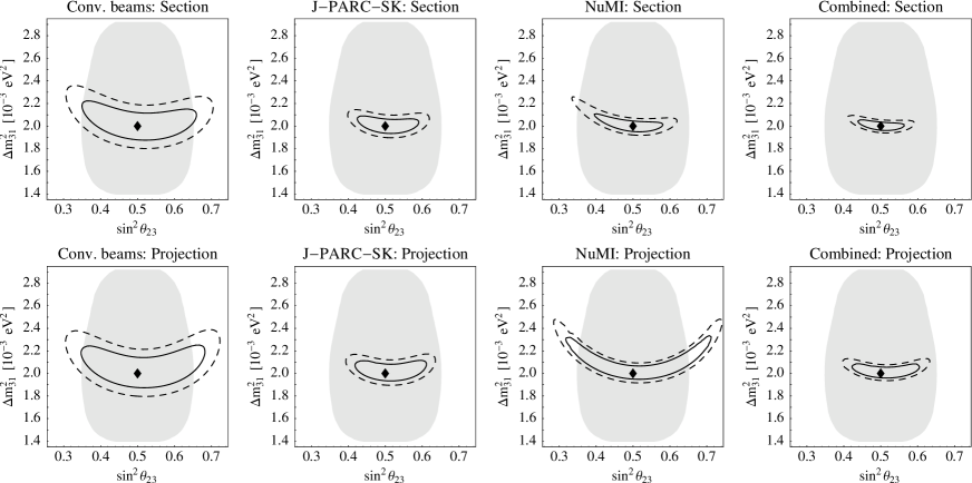
Figure 1: The $90\%$ CL (solid curves) and $3\sigma$ (dashed curves) allowed regions (2 d.o.f.) in the $\sin^{2}\theta_{23}$-$\Delta m_{31}^{2}$-plane for the combined conventional beams (MINOS, ICARUS, OPERA), JPARC-SK, NuMI, and all beam experiments combined. For the true values of the oscillation parameters, we choose the current best-fit values from Eq. (3), a normal mass hierarchy, $\sin^{2}2\theta_{13}=0.1$ and $\delta_{\mathrm{CP}}=0$. The upper row shows a section of the fit manifold (with the un-displayed oscillation parameters fixed at their true values), and the lower row shows the projection onto the $\sin^{2}\theta_{23}$-$\Delta m_{31}^{2}$-plane as the final result. The shaded regions correspond to the 90% CL allowed region from current atmospheric neutrino data [2].

The first thing to learn from Figure 1 is that the precision on $\Delta m_{31}^{2}$ will drastically improve during the next ten years, whereas our knowledge on $\theta_{23}$ will be increased rather modestly. The combination of all the beam experiments will improve the current precision from the Super-Kamiokande atmospheric neutrino data [2] on $\sin^{2}\theta_{23}$ roughly by a factor of two, while the precision on $\Delta m_{31}^{2}$ will be improved by an order of magnitude. Neither the three conventional beams combined nor NuMI will obtain a precision on $\theta_{23}$ better than current Super-Kamiokande data, only JPARC-SK might improve the precision slightly. We note however, that the $\theta_{23}$ accuracy of the long-baseline experiments strongly depends on the true value of $\Delta m_{31}^{2}$, and it will be improved if $\Delta m_{31}^{2}$ turns out to be larger than the current best-fit point.

In most cases, the correlations with the un-displayed oscillation parameters do not cause significant differences between the sections and projections in the upper and lower rows of Figure 1. Only for NuMI, the projection is affected by the multi-parameter correlation with $\sin^{2}2\theta_{13}$ and $\delta_{\mathrm{CP}}$. Since we do not assume additional knowledge about $\sin^{2}2\theta_{13}$ for the individual experiments other than from their own appearance channels, the appearance channels can indirectly affect the $\Delta m_{31}^{2}$ or $\theta_{23}$ measurement results. This can be understood in terms of the disappearance probability, which to leading order is given by [35, 36]

$$P_{\mu\mu}=1-\sin^{2}2\theta_{23}\sin^{2}\frac{\Delta m_{31}^{2}L}{4E}+\ldots$$ (5)

where the dots refer to higher order terms in $\alpha=\Delta m_{21}^{2}/\Delta m_{31}^{2}$ and $\theta_{13}$, as well as products of these. Thus, the $\sin^{2}2\theta_{13}$-precision, which comes from the appearance channels, is necessary to constrain the amplitude of the higher order terms in this equation which are proportional to $\theta_{13}$. Since, however, $\theta_{13}$ is strongly correlated with $\delta_{\mathrm{CP}}$ in the appearance channels, this two-parameter correlation can lead to multi-parameter correlations with $\theta_{23}$ or $\Delta m_{31}^{2}$ in the disappearance channel through the higher order terms in Eq. (5). This explains the small differences between the section and projection plots in Figure 1. In addition, the measurement of $\sin^{2}2\theta_{13}$ at NuMI is affected by matter effects, and hence, is somewhat different for the opposite sign of $\Delta m_{31}^{2}$. Therefore, one can also expect a slightly different shape of the fit manifold for the $\mathrm{sgn}(\Delta m_{31}^{2})$-degeneracy. Note that the initial asymmetry between $\sin^{2}\theta_{23}<0.5$ and $\sin^{2}\theta_{23}>0.5$ for NuMI is caused by its large matter effects.

Eventually, one obtains the precision of the individual parameter $\Delta m_{31}^{2}$ or $\theta_{23}$ as projection of the lower row plots in Figure 1 (for one degree of freedom) onto the respective axis. In Table 2 we show our prediction for the $3\sigma$-allowed ranges of the atmospheric oscillation parameters from the conventional beam experiments and first generation superbeam experiments for one degree of freedom.

Experiment/Combination	$|\Delta m_{31}^{2}|$	$\theta_{23}$	$\sin^{2}\theta_{23}$
MINOS + OPERA + ICARUS	$2^{+0.34}_{-0.18}\cdot 10^{-3}\,\mathrm{eV}^{2}$	$(\pi/4)^{+0.22}_{-0.19}$	$0.5^{+0.21}_{-0.18}$
JPARC-SK	$2^{+0.15}_{-0.09}\cdot 10^{-3}\,\mathrm{eV}^{2}$	$(\pi/4)^{+0.13}_{-0.10}$	$0.5^{+0.13}_{-0.10}$
NuMI	$2^{+0.43}_{-0.07}\cdot 10^{-3}\,\mathrm{eV}^{2}$	$(\pi/4)^{+0.24}_{-0.21}$	$0.5^{+0.23}_{-0.20}$
All beam experiments combined	$2^{+0.12}_{-0.06}\cdot 10^{-3}\,\mathrm{eV}^{2}$	$(\pi/4)^{+0.13}_{-0.10}$	$0.5^{+0.12}_{-0.09}$

Table 2: The expected allowed ranges ($3\sigma$, 1 d.o.f.) for the atmospheric oscillation parameters. For the true values of the oscillation parameters, we choose the current best-fit values, a normal mass hierarchy, $\sin^{2}2\theta_{13}=0.1$, and $\delta_{\mathrm{CP}}=0^{\circ}$. The impact of an inverted mass hierarchy, and different values for $\sin^{2}2\theta_{13}$ or $\delta_{\mathrm{CP}}$ on these final results is rather small.

5 Improved $\boldsymbol{\sin^{2}2\theta_{13}}$ bounds from conventional beams

Let us now come to the crucial next step in neutrino oscillation physics: the determination of the small mixing angle $\theta_{13}$. We start this discussion by investigating the potential of the conventional beam experiments MINOS, ICARUS, and OPERA to improve the current bound on $\sin^{2}2\theta_{13}$.

In Table 3, we show the signal and background event rates after one year of nominal operation for each experiment (computed for $\sin^{2}2\theta_{13}=0.1$ and $\delta=0$). Based on these numbers, one would expect that MINOS performs significantly better than ICARUS. However, Table 3 only shows integrated event rates and does not include the energy dependence of signal versus background event numbers. In the CNGS beam, the energy distribution of the intrinsic $\nu_{e}$-contamination is rather different from the energy distribution of the signal events. Thus, in a full analysis including energy information, the impact of the background is reduced. On the other hand, for the NuMI neutrino beam, the intrinsic $\nu_{e}$-contamination has an energy distribution which is much closer to the one of the signal events. Therefore, the impact of the background is relatively high.

	MINOS	ICARUS	OPERA
Signal	7.1	4.4	1.6
Background	21.6	12.2	5.4
S/B	0.33	0.36	0.30

Table 3: The number of signal and background events after one year of nominal operation of MINOS, ICARUS, and OPERA. For the oscillation parameters, we use the current best-fit values with $\sin^{2}2\theta_{13}=0.1$, $\delta_{\mathrm{CP}}=0$, and a normal mass hierarchy.

An important issue for the $\sin^{2}2\theta_{13}$ sensitivity limit from the conventional beams is the finally achieved integrated luminosity, which might differ significantly from the nominal value due to some unforeseen experimental circumstances. Therefore, we discuss the $\sin^{2}2\theta_{13}$ sensitivity as a function of the integrated number of protons on target. In Figure 2, the sensitivity limits for MINOS, ICARUS, and OPERA are shown as a function of the luminosity. Note that since the CNGS experiments will be running simultaneously, we also show the combined ICARUS and OPERA sensitivity limit. In order to compare the achievable limits as a function of the running time, the dashed lines refer to the results after one, two, and five years of data taking with the nominal beam fluxes given in Refs. [44, 12, 45]. The lowest curves are obtained for the statistics limits only, whereas the highest curves are obtained after successively switching on systematics, correlations, and degeneracies. Thus, the actual $\sin^{2}2\theta_{13}$ sensitivity limit in Figure 2 is given by the highest curves. The figure indicates that the CNGS experiments together can improve the CHOOZ bound after about one and a half years of running time, and MINOS after about two years. We note that the impact of systematics increases for MINOS with increasing luminosity, illustrating the typical background problem mentioned above. In Figure 3, we eventually summarize the $\sin^{2}2\theta_{13}$ sensitivity after a total running time of five years for each experiment, assuming the true value of $\Delta m_{31}^{2}=2\cdot 10^{-3}\,\mathrm{eV}^{2}$. One can directly read off this figure that the $\sin^{2}2\theta_{13}$ sensitivity limits of ICARUS and MINOS are very similar, and ICARUS and OPERA combined are slightly better than MINOS.

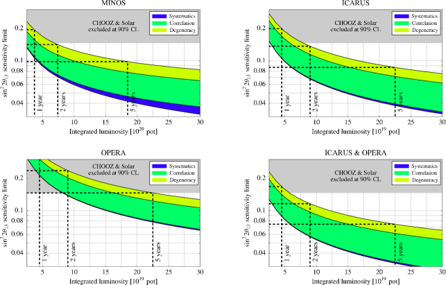
Figure 2: The $\sin^{2}2\theta_{13}$ sensitivity limit as function of the total number of protons on target at the 90% confidence level for MINOS, ICARUS, OPERA, and ICARUS and OPERA combined (5% flux uncertainty assumed). The dashed curves refer to the sensitivity limits after one, two, and five years of running. The lowest curves are obtained for the statistics limits only, whereas the highest curves are obtained after successively switching on systematics, correlations, and degeneracies, i.e., they correspond to the final sensitivity limits. The gray-shaded area shows the current $\sin^{2}2\theta_{13}$ excluded region $\sin^{2}2\theta_{13}\gtrsim 0.14$ at the 90% CL [42]. For the true values of the oscillation parameters we use the current best-fit values Eq. (3) and a normal mass hierarchy.

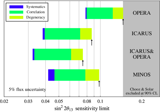
Figure 3: The $\sin^{2}2\theta_{13}$ sensitivity limit at the 90% confidence level after a running time of five years for the different experiments. The left edges of the bars are obtained for the statistics limits only, whereas the right edges are obtained after successively switching on systematics, correlations, and degeneracies, i.e., they correspond to the final $\sin^{2}2\theta_{13}$ sensitivity limits. The gray-shaded area shows the current $\sin^{2}2\theta_{13}$ excluded region $\sin^{2}2\theta_{13}\gtrsim 0.14$ at the 90% CL [42]. For the true values of the oscillation parameters, we use the current best-fit values Eq. (3) and a normal mass hierarchy.

Let us briefly compare our results to $\sin^{2}2\theta_{13}$ sensitivity limit calculations for MINOS, ICARUS, and OPERA existing in the literature. In the analysis of Ref. [46], the correlation with $\delta_{\mathrm{CP}}$ and the sign($\Delta m_{31}^{2}$)-degeneracy are included, and hence these results should be compared with our final sensitivity limits, although we also include correlations with respect to all the other oscillation parameters. However, for the comparison, one has to take into account the different considered running times for MINOS (2 years vs. 5 years), as well as the difference in the chosen true value of $|\Delta m_{31}^{2}|$ ($3.0\cdot 10^{-3}\,\mathrm{eV}^{2}$ vs. $2.0\cdot 10^{-3}\,\mathrm{eV}^{2}$). In the analysis performed in Ref. [47], the correlation with $\delta_{\mathrm{CP}}$ and the sign($\Delta m_{31}^{2}$)-degeneracy were not considered, while correlations with $|\Delta m^{2}_{31}|$ were taken into account. Therefore, the results from that study should roughly be compared to our $(\sin^{2}2\theta_{13})_{\mathrm{eff}}$ limits. Again one has to take into account different assumptions about the running times and the true value for $\Delta m^{2}_{21}$ ($5.0\cdot 10^{-5}\,\mathrm{eV}^{2}$ vs. $7.0\cdot 10^{-5}\,\mathrm{eV}^{2}$). Finally, in Appendix A.2 we demonstrate explicitly that our results are in excellent agreement with the ones obtained by the MINOS, ICARUS, and OPERA collaborations [44, 12, 45] if we use the same assumptions.

A very interesting issue for the conventional beam experiments is the impact of the true value of $\Delta m_{21}^{2}$ on the $\sin^{2}2\theta_{13}$ sensitivity. (The impact of the true value of $\Delta m_{31}^{2}$ is discussed in Section 6.) One can easily see from Eq. (1) that the effect of $\delta_{\mathrm{CP}}$ increases with increasing $\alpha\equiv\Delta m_{21}^{2}/\Delta m_{31}^{2}$, which determines the amplitude of the second and third terms in this equation. Since the main contribution to the correlation part of the discussed figures comes from the correlation with $\delta_{\mathrm{CP}}$ (with some contribution of the uncertainty of the solar parameters), a larger $\Delta m_{21}^{2}$ causes a larger correlation bar. This can clearly by seen from Figure 4, which shows the combined potential of the conventional beams after five years of running time (for each experiment) as a function of $\Delta m_{21}^{2}$. In this figure the right edge of the blue band corresponds to the limit based only on statistical and systematical errors, i.e., the $(\sin^{2}2\theta_{13})_{\mathrm{eff}}$ sensitivity limit. We find that the larger $\Delta m_{21}^{2}$ is, the better becomes the systematics-based $(\sin^{2}2\theta_{13})_{\mathrm{eff}}$ sensitivity limit, and the worse becomes the final sensitivity limit on $\sin^{2}2\theta_{13}$. Since the LMA-II region is now disfavored by the latest solar neutrino and KamLAND data, Figure 4 demonstrates that the conventional beam experiments can definitively improve the current $\sin^{2}2\theta_{13}$-bound. One may expect an improvement down to $\sin^{2}2\theta_{13}\lesssim 0.05-0.07$ within the LMA-I allowed region, where the $\sin^{2}2\theta_{13}$ sensitivity limit at the current best-fit value is about $\sin^{2}2\theta_{13}\leq 0.06$.

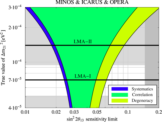
Figure 4: The $\sin^{2}2\theta_{13}$ sensitivity limit at 90% CL for MINOS, ICARUS, and OPERA combined as function of the true value of $\Delta m_{21}^{2}$ (five years running time). The left curve is obtained for the statistics limit only, whereas the right curve is obtained after successively switching on systematics, correlations, and degeneracies, i.e., it corresponds to the final $\sin^{2}2\theta_{13}$ sensitivity limit. The dark gray-shaded area shows the current $\sin^{2}2\theta_{13}$ excluded region $\sin^{2}2\theta_{13}\gtrsim 0.14$ at the 90% CL, and the light gray-shaded area refers to the LMA-excluded region at $3\sigma$, where the best-fit value is marked by the horizontal line [42]. For the true values of the un-displayed oscillation parameters we use the current best-fit values in Eq. (3) and a normal mass hierarchy.

Since the $\sin^{2}2\theta_{13}$ sensitivity limit is expected to be $\sin^{2}2\theta_{13}\leq 0.06$ for MINOS, ICARUS, and OPERA combined (with five years running time for each experiment), a further improvement from the conventional beams seems to be unlikely. In addition, the systematics limitation, which can be clearly seen in Figure 2, demonstrates that a further increase of the luminosity would not lead to significantly better bounds on $\sin^{2}2\theta_{13}$. Therefore, one has to proceed to the next generation of experiments to increase the $\sin^{2}2\theta_{13}$ sensitivity. Especially, the off-axis technology to suppress backgrounds and more optimized detectors could help to improve the performance. Amongst other experiments, we discuss the corresponding superbeams, which are using these improvements, in the next section.

6 Further improvement of the $\boldsymbol{\sin^{2}2\theta_{13}}$ bound

After the discussion of the conventional beams in the last section, we here discuss the final bound on $\sin^{2}2\theta_{13}$ in ten years from now, if no finite value will be found (we will in the next section consider the case of a large $\theta_{13}$). We first discuss in Section 6.1 the potential of a new reactor neutrino experiment, whereas we compare in Section 6.2 the $\sin^{2}2\theta_{13}$ limits from conventional beams, reactor experiments, and superbeams.

6.1 Characteristics of reactor neutrino experiments

In Figure 5, we show the $\sin^{2}2\theta_{13}$ sensitivity from reactor neutrino experiments as a function of the integrated luminosity measured in t (fiducial far detector mass) $\times$ GW (thermal reactor power) $\times$ yr (time of data taking). We consider two options of the far detector baseline: $L_{\mathrm{FD}}=1.05\,\mathrm{km}$, corresponding to the baseline of the CHOOZ site, and $L_{\mathrm{FD}}=1.7\,\mathrm{km}$, which is optimized for values of $\Delta m^{2}_{31}\sim(2-4)\cdot 10^{-3}\,\mathrm{eV}^{2}$ [20]. A crucial parameter for the $\sin^{2}2\theta_{13}$ sensitivity is the uncertainty of the relative normalization between the near and far detectors. We show the sensitivity for two representative values for this relative normalization uncertainty: First, $\sigma_{\mathrm{rel}}=0.6\%$ is a realistic value for two identical detectors [23]. Second, in order to illustrate the improvement of the performance of an reactor experiment with a reduced normalization error, we consider the very optimistic assumption of $\sigma_{\mathrm{rel}}=0.2\%$. Such a small value might be achievable with movable detectors, as discussed for some proposals in the US [24]. The shaded regions in Figure 5 correspond to the range of possible sensitivity limits for different assumptions of systematical errors and backgrounds. For the optimal case (lower curves), we only include the absolute flux and relative detector uncertainties $\sigma_{\mathrm{abs}}$ and $\sigma_{\mathrm{rel}}$. For the worst limits (upper curves) we include in addition an error on the spectral shape $\sigma_{\mathrm{shape}}=2\%$, the energy scale uncertainty $\sigma_{\mathrm{cal}}=0.5\%$, and various backgrounds as discussed in Appendix B.

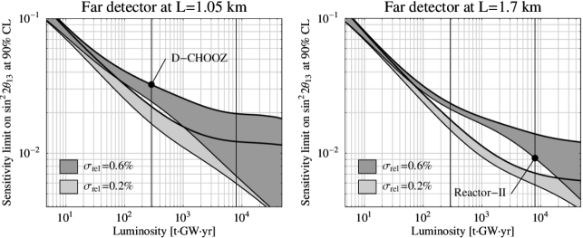
Figure 5: Luminosity scaling of the $\sin^{2}2\theta_{13}$ sensitivity at the 90% CL. Here $\Delta m_{31}^{2}=2\cdot 10^{-3}$ eV² is assumed to be known within 5%, $L_{\mathrm{ND}}=0.15\,\mathrm{km}$, and $L_{\mathrm{FD}}=1.05\,(1.7)\,\mathrm{km}$ in the left (right) panel. The number of events in the near detector is fixed to $2.94\cdot 10^{6}$. We use $\sigma_{\mathrm{abs}}=2.5\%$ and $\sigma_{\mathrm{rel}}=0.2\%\,(0.6\%)$ for the light (dark) shaded regions. The upper edge of each region is calculated for $\sigma_{\mathrm{shape}}=2\%$, $\sigma_{\mathrm{cal}}=0.5\%$, and backgrounds as given in Table 6 in Appendix B. For the lower edges, we set $\sigma_{\mathrm{shape}}=\sigma_{\mathrm{cal}}=0$ and do not include backgrounds. The dots mark the Double-Chooz and Reactor-II setups.

The first observation from Figure 5 is that the shaded regions in the left-hand panel are significantly wider than in the right-hand panel, which demonstrates that a reactor experiment at $1.05\,\mathrm{km}$ is more sensitive to systematical errors. This reflects the fact that the baseline of $1.7\,\mathrm{km}$ is better optimized for the used value of $|\Delta m_{31}^{2}|=2\cdot 10^{-3}\,\mathrm{eV}^{2}$, such that the oscillation minimum is well contained in the center of the observed energy range. In contrast, for the baseline of $1.05\,\mathrm{km}$, the signal is shifted to the low energy edge of the spectrum. This implies that the interplay of background uncertainties, energy calibration, and shape error has a larger impact on the final sensitivity limit.

However, from the left-hand panel, one finds that for experiments of the size of Double-Chooz, the impact of systematics is rather modest; the $\sin^{2}2\theta_{13}$ sensitivity of 0.024 for normalization errors only deteriorates to 0.032 if all systematics errors and backgrounds are included. We conclude that the proposed Double-Chooz project is rather insensitive to systematical effects and will be able to provide a robust limit $\sin^{2}2\theta_{13}\lesssim 0.032$, although the far detector baseline is not optimized. In contrast, if one aims at higher luminosities, the systematics will have to be well under control at a non-optimal baseline such as at the CHOOZ site. In that case, it is saver to use a longer baseline. We note that the main limiting factor for large luminosities in the right-hand panel of Figure 5 is the error on a bin-to-bin uncorrelated background. Furthermore, comparing the light and dark shaded regions in that plot, it is obvious that a smaller relative normalization error will significantly improve the performance of a large experiment at $1.7\,\mathrm{km}$, and will further reduce the impact of systematics and backgrounds. With the ambitious value of $\sigma_{\mathrm{rel}}=0.2\%$, sensitivity limits of $\sin^{2}2\theta_{13}\lesssim 7\cdot 10^{-3}$ could be obtained with a Reactor-II-type experiment.

Eventually, we have demonstrated that the Double-Chooz experiment could give a robust $\sin^{2}2\theta_{13}$ sensitivity limit. In fact, one can read off Figure 5 (D-Chooz-dot) that our assumptions about Double-Chooz are rather conservative. Since a Letter of Intent for this experiment is in preparation, we use it in the next subsection for a direct quantitative comparison to the superbeams. However, as one can also learn from Figure 5, luminosity and different systematics sources are important issues for a reactor experiment. Therefore, one should keep in mind that much better $\sin^{2}2\theta_{13}$ sensitivity limits could be obtained from reactor experiments, such as the Reactor-II setup. However, the exact final sensitivity limits will in these cases depend on many sources, which means that they are hardly predictable right now.

6.2 The $\boldsymbol{\sin^{2}2\theta_{13}}$ bound from different experiments in ten years from now

Let us now assume that the conventional beam experiments MINOS, ICARUS, and OPERA have been running five years each, and that the Double-Chooz experiment has accumulated three years of data. In addition, we assume that the superbeam experiments JPARC-SK and NuMI have reached the integrated luminosities as given in Table 1. (For earlier, more extensive discussions of the potential of superbeam experiments, we refer to Ref. [26].)

In Figure 6, we show the $\sin^{2}2\theta_{13}$ sensitivity for the considered experiments. The final sensitivity limit is obtained after successively switching on systematics, correlations, and degeneracies as the rightmost edge of the bars. Figure 6 demonstrates that the beam experiments are dominated by correlations and degeneracies, whereas the reactor experiments are dominated by systematics. It can be clearly seen that the $(\sin^{2}2\theta_{13})_{\mathrm{eff}}$ sensitivity limit (between systematics and correlation bar), or the precision of a combination of parameters leading to a positive signal, is much better for the superbeams than for the reactor experiments. Therefore, though the reactor experiments have a good potential to extract $\sin^{2}2\theta_{13}$ directly, the superbeams results will in addition contain a lot of indirect information about $\delta_{\mathrm{CP}}$ and the mass hierarchy, which might be resolved by the combination with complementary information. We call this gain in the physics potential which goes beyond the simple addition of statistics for the combination of experiments “synergy”. In Section 7, we will discuss this further for the case if $\sin^{2}2\theta_{13}$ turns out to be large.

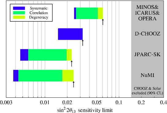
Figure 6: The $\sin^{2}2\theta_{13}$ sensitivity limit at the 90% CL for MINOS, ICARUS, and OPERA combined, Double-Chooz, JPARC-SK, and NuMI. The left edges of the bars are obtained for the statistics limits only, whereas the right edges are obtained after successively switching on systematics, correlations, and degeneracies, i.e., they correspond to the final $\sin^{2}2\theta_{13}$ sensitivity limits. The gray-shaded region corresponds to the current $\sin^{2}2\theta_{13}$ bound at 90% CL. For the true values of the oscillation parameters, we use the current best-fit values in Eq. (3) and a normal mass hierarchy.

Another conclusion from Figure 6 is that it is very important to compare the $\sin^{2}2\theta_{13}$ sensitivities of different experiments which are obtained with equal methods. In particular one clearly has to distinguish between the $(\sin^{2}2\theta_{13})_{\mathrm{eff}}$ sensitivity limit (between systematics and correlation bar) and the final $\sin^{2}2\theta_{13}$ sensitivity limit, including correlations and degeneracies. For example, by accident the $(\sin^{2}2\theta_{13})_{\mathrm{eff}}$ sensitivity limit from the combined MINOS, ICARUS, and OPERA experiments is very close to the final sensitivity limit of JPARC-SK or NuMI. Thus, one may end up with two similar numbers, which however, refer to different quantities and are not comparable.

A very important parameter for future $\sin^{2}2\theta_{13}$ measurements is the true value of $\Delta m_{31}^{2}$, which currently is constrained to the interval $0.0011\,\mathrm{eV}^{2}\lesssim|\Delta m_{31}^{2}|\lesssim 0.0032\,\mathrm{eV}^{2}$ at $3\sigma$ [2]. From Figure 7, one can can easily see that the true value of $\Delta m_{31}^{2}$ strongly affects the $\sin^{2}2\theta_{13}$ sensitivity limit. The left-hand plot in this figure demonstrates that for all experiments the $\sin^{2}2\theta_{13}$ sensitivity becomes worse for small values of $|\Delta m_{31}^{2}|$ within the currently allowed range. However, since also the current $\sin^{2}2\theta_{13}$ bound (dark-gray shaded region) is worse for small values of $|\Delta m_{31}^{2}|$ than for large values, the relative improvement of the current $\sin^{2}2\theta_{13}$ bound might be a more appropriate description of the experiment performance. This relative improvement as function of the true value of $|\Delta m_{31}^{2}|$ is shown in the right-hand plot of Figure 7, where a factor of unity corresponds to no improvement. From this plot, one can read off an improvement by a factor of two for the conventional beams, a factor of four for Double-Chooz, and a factor of six for the superbeams at the atmospheric best-fit value (vertical line). Nevertheless, the conventional beams might not improve the current bound at all for small values of $|\Delta m_{31}^{2}|$ within the atmospheric allowed range, whereas any of the other experiments would improve the current bound at least by a factor of two. Thus, though the $\sin^{2}2\theta_{13}$ sensitivity limit could be as be as large as $\sin^{2}2\theta_{13}\lesssim 0.1$ for small values of $|\Delta m_{31}^{2}|$ for the superbeams or Double-Chooz, those experiments would still improve the current bound by a factor of two.

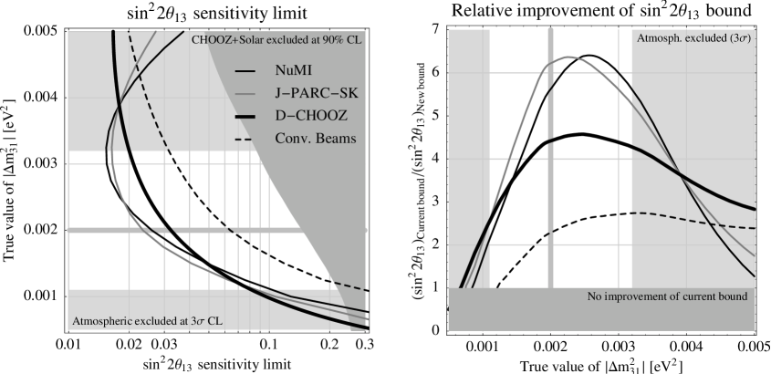
Figure 7: Left panel: The $\sin^{2}2\theta_{13}$ sensitivity limits at 90% CL from the experiments NuMI, JPARC-SK, Double-Chooz, and the combined conventional beams (MINOS, ICARUS, OPERA) as function of the true value of $|\Delta m_{31}^{2}|$. The dark-gray shaded region refers to the current $\sin^{2}2\theta_{13}$ bound from CHOOZ and the solar experiments (90% CL) [42]. Right panel: The relative improvement of the $\sin^{2}2\theta_{13}$ sensitivity limit with respect to the current bound from CHOOZ and solar experiments, where the dark-gray region corresponds to no improvement. The light-gray shaded regions in both panels refer to the atmospheric excluded regions ($3\sigma$), and the lines in the middle mark the current atmospheric best-fit value.

7 Opportunities if $\boldsymbol{\sin^{2}2\theta_{13}}$ is just around the corner

In Section 6, we have discussed how much the $\sin^{2}2\theta_{13}$ bound could be improved if the true value of $\sin^{2}2\theta_{13}$ were zero. There are, however, very good theoretical reasons to expect $\sin^{2}2\theta_{13}$ to be finite, such that the experiments under consideration could establish $\sin^{2}2\theta_{13}>0$. In this case, one could aim for the $\sin^{2}2\theta_{13}$ precision, CP violation, CP precision measurements, and the mass hierarchy determination. Though it has been shown that CP and mass hierarchy measurements are very difficult for the first-generation superbeams and new reactor experiments [19, 27, 26, 20, 48], we will demonstrate in this section that we could still learn something about these parameters if $\sin^{2}2\theta_{13}$ turns out to be large. In particular, we discuss the combination of the discussed experiments for the case $\sin^{2}2\theta_{13}=0.1$. This would imply that a positive $\sin^{2}2\theta_{13}$ signal could already be seen with the next generation of experiments. As discussed in Section 2, we assume here that a large reactor experiment Reactor-II will be available at the end of the period under consideration to resolve the correlation between $\sin^{2}2\theta_{13}$ and $\delta_{\mathrm{CP}}$. We note again that similar results can be obtained by the superbeams in the antineutrino mode using higher target powers or detector upgrades.

The superbeam appearance channels will lead to allowed regions in the $\sin^{2}2\theta_{13}$-$\delta_{\mathrm{CP}}$-plane, similar to the allowed regions for solar and atmospheric oscillation parameters from current data. We show the results of JPARC-SK, NuMI, and Reactor-II for the true values $\sin^{2}2\theta_{13}=0.1$ and $\delta_{\mathrm{CP}}=90^{\circ}$ in Figure 8, and $\delta_{\mathrm{CP}}=-90^{\circ}$ in Figure 9. For the right-most plots in these figures, we combine all experiments including the conventional beams MINOS, ICARUS, and OPERA, although they do not contribute significantly to the final result. Since we assume a normal mass hierarchy to generate the data, the best-fit is obtained by fitting with the normal hierarchy; the corresponding regions are shown by the black curves. The $\mathrm{sgn}(\Delta m_{31}^{2})$-degenerate regions are obtained by fitting the data assuming an inverted hierarchy (gray curves). Thus, the best-fit and degenerate manifolds, which are disconnected in the six-dimensional parameter space, are shown in the same plots. Similar to Figure 1 we demonstrate the difference between a section of the fit manifold (upper rows) and a projection (lower rows) in these figures.

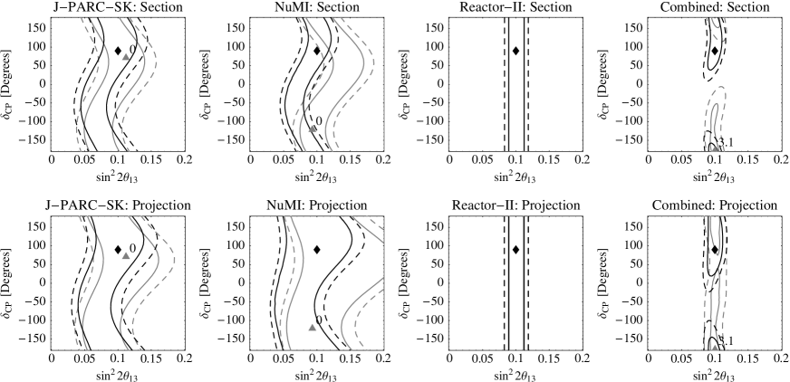
Figure 8: The $90\%$ CL (solid curves) and $3\sigma$ (dashed curves) allowed regions (2 d.o.f.) in the $\sin^{2}2\theta_{13}$-$\delta_{\mathrm{CP}}$-plane for the true values $\sin^{2}2\theta_{13}=0.1$ and $\delta_{\mathrm{CP}}=90^{\circ}$ for JPARC-SK, NuMI, Reactor-II. The right-most plots are calculated for the shown experiments in combination with the conventional beams. For the true values of the un-displayed oscillation parameters, we choose the current best-fit values and a normal mass hierarchy. The black curves refer to the allowed regions for the normal mass hierarchy, whereas the gray curves refer to the $\mathrm{sgn}(\Delta m_{31}^{2})$-degenerate solution (inverted hierarchy), where the projections of the minima onto the $\sin^{2}2\theta_{13}$-$\delta_{\mathrm{CP}}$-plane are shown as diamonds (normal hierarchy) and triangles (inverted hierarchy). For the latter, the $\Delta\chi^{2}$-value with respect to the best-fit point is also given. The upper row shows the fit manifold section (with the un-displayed oscillation parameters fixed at their true values), and the lower row shows the projection onto the $\sin^{2}2\theta_{13}$-$\delta_{\mathrm{CP}}$-plane as the final result.

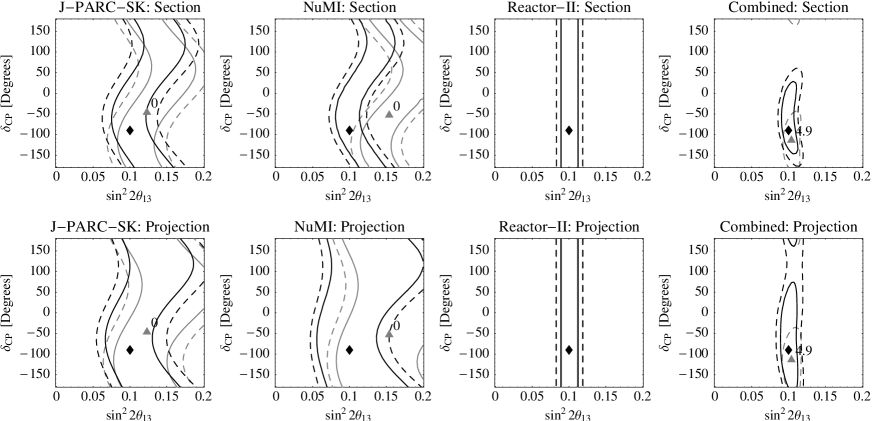
Figure 9: The same as Figure 8 but for the true value $\delta_{\mathrm{CP}}=-90^{\circ}$.

As far as the measurement of $\sin^{2}2\theta_{13}$ is concerned, any of the experiments in Figures 8 and 9 can establish $\sin^{2}2\theta_{13}>0$ for $\sin^{2}2\theta_{13}=0.1$ at $3\sigma$. The $\sin^{2}2\theta_{13}$-precision can be read off from the figures as projection of the bands onto the $\sin^{2}2\theta_{13}$-axis. The band structures of JPARC-SK and NuMI come from the CP phase dependency in Eq. (1). Because of the larger matter effects, the degenerate solution for NuMI is rather different from the best-fit solution, whereas it is very similar to the best-fit solution for JPARC-SK. For Reactor-II, the $\sin^{2}2\theta_{13}$-precision can be read off directly, since a reactor experiment is not affected by $\delta_{\mathrm{CP}}$ (see Eq. (2)), and the mass hierarchy has essentially no effect. Note that the treatment of the $\mathrm{sgn}(\Delta m_{31}^{2})$-degeneracy in such a situation as shown in Figures 8 and 9 is a matter of definition: One could either return two different intervals for normal and inverted mass hierarchies, or one could return the union of the two fit intervals as more condensed information.

The figures show that for $\delta_{\mathrm{CP}}$, none of the individual experiments can give any information, since no substantial fraction of antineutrino running is involved. However, there is some information on $\delta_{\mathrm{CP}}$ for the combination of all experiments, since the complementary information from the reactor experiment helps to resolve the superbeam bands. Note that the overall performance for the considered experiments (including the $\mathrm{sgn}(\Delta m_{31}^{2})$-degeneracy) is usually better close to the true value $\delta_{\mathrm{CP}}=-90^{\circ}$ than close to the true value $\delta_{\mathrm{CP}}=90^{\circ}$, since the degeneracy includes for $\delta_{\mathrm{CP}}=90^{\circ}$ very different values of $\delta_{\mathrm{CP}}$ far away from the best-fit manifold. This can, for example, be understood in terms of bi-rate graphs (cf., Refs. [38, 48]). From a separate analysis of the CP precision, we find that one could exclude as much as up to 40% of all values of $\delta_{\mathrm{CP}}$ at the $90\%$ confidence level (1 d.o.f., close to $\delta_{\mathrm{CP}}=-90^{\circ}$). However, if $\delta_{\mathrm{CP}}$ turns out to be close to $0$ or $\pi$, we find that one could not obtain any information on $\delta_{\mathrm{CP}}$. Furthermore, one can directly read off from Figures 8 and 9 that CP violation measurements will not be possible with the considered experiments at the $90\%$ confidence level (2 d.o.f. in these figures), since for the true values $\delta_{\mathrm{CP}}=\pm 90^{\circ}$ corresponding to maximal CP violation, the projected allowed regions (even the best-fit solutions) include at least one of the CP conserving cases $\delta_{\mathrm{CP}}\in\{0,180^{\circ}\}$. One can show that even for one degree of freedom, there is no CP violation sensitivity with the discussed experiments at the $90\%$ confidence level.

Another important issue for the next generation long-baseline experiments is the mass hierarchy determination. In Figures 8 and 9 we give the $\Delta\chi^{2}$-values for the minimum in the fit manifold corresponding to the $\mathrm{sgn}(\Delta m_{31}^{2})$-degenerate solution (i.e., for the inverted mass hierarchy) with respect to the best-fit minimum for the normal hierarchy ($\Delta\chi^{2}=0$), which is the relevant number for the sensitivity to a normal mass hierarchy. Obviously, none of the individual experiments has a mass hierarchy sensitivity, but their combination has some. The mass hierarchy sensitivity becomes only possible because of the long NuMI baseline $L=812\,\mathrm{km}$ [29, 26, 30], since matter effects differ for the normal and inverted mass hierarchies. Eventually, a NuMI baseline even longer than $L=812\,\mathrm{km}$ could further improve the mass hierarchy sensitivity [26, 48]. We note that the ability to identify the mass hierarchy strongly depends on the (unknown) true value of $\delta_{\mathrm{CP}}$. The mass hierarchy determination at the combined superbeams is close to the optimum for $\delta_{\mathrm{CP}}=-90^{\circ}$, and close to the minimum for $\delta_{\mathrm{CP}}=90^{\circ}$ [38, 48]. In fact, one could have a better sensitivity to the normal mass hierarchy for $\delta_{\mathrm{CP}}=-90^{\circ}$ ($\Delta\chi^{2}=4.9$, see Figure 9) than for $\delta_{\mathrm{CP}}=90^{\circ}$ ($\Delta\chi^{2}=3.1$, see Figure 8) at the $90\%$ confidence level ($\Delta\chi^{2}=2.71$ for 1 d.o.f.).

8 Summary and conclusions

This study has focused on the future neutrino oscillation long-baseline experiments on a timescale of about ten years. The primary objective has been the search for $\sin^{2}2\theta_{13}$, but we have also analyzed the “atmospheric” parameters $\theta_{23}$ and $\Delta m_{31}^{2}$. The main selection criterion for the different experiments has been the availability of specific studies, such as LOIs or proposals, or that they are even being under construction. We assume that an experiment (including data taking and analysis) will only be feasible within the coming ten years, if it is already now actively being planned. The next long-baseline experiments will be the conventional beam experiments MINOS, ICARUS, and OPERA  which are currently under construction. In addition, the JPARC-SK and NuMI superbeam experiments are under active consideration with existing proposals and will most likely provide results within the next ten years. Furthermore, new reactor neutrino experiments are actively being discussed. In this study, we have considered the Double-Chooz project, which will probably deliver results in the anticipated timescale, since infrastructure (such as the detector cavity) of the original CHOOZ experiment can be re-used.

First, we have investigated the possible improvement of our knowledge on the leading atmospheric oscillation parameters. We have found that the conventional beams and superbeams will reduce the error on $\Delta m_{31}^{2}$ by roughly an order of magnitude within the next ten years. The precision of $\theta_{23}$ is dominated by JPARC-SK and will improve only by a factor of two (cf., Table 4).

	Current	Beams	D-Chooz	JPARC-SK	NuMI	Reactor-II	Comb.
$\sin^{2}2\theta_{13}$ sensitivity limit (90% CL)
$\sin^{2}2\theta_{13}$	0.14	0.061	0.032	0.023	0.024	(0.009)	(0.009)
$(\sin^{2}2\theta_{13})_{\mathrm{eff}}$	0.14	0.026	0.032	0.006	0.004	(0.009)	(0.003)
Allowed ranges for leading atmospheric parameters ($3\sigma$)
$\frac{|\Delta m_{31}^{2}|}{10^{-3}\,\mathrm{eV}^{2}}$	2${}^{+1.2}_{-0.9}$	2${}^{+0.34}_{-0.18}$	$-$	2${}^{\boldsymbol{+0.15}}_{-0.09}$	2${}^{+0.43}_{\boldsymbol{-0.07}}$	$-$	2${}^{+0.12}_{-0.06}$
$\theta_{23}$	$(\frac{\pi}{4})^{+0.20}_{-0.20}$	$(\frac{\pi}{4})^{+0.22}_{-0.19}$	$-$	$(\frac{\pi}{4})\boldsymbol{{}^{+0.13}_{-0.10}}$	$(\frac{\pi}{4})^{+0.24}_{-0.21}$	$-$	$(\frac{\pi}{4})^{+0.13}_{-0.10}$
Measurements for large $\sin^{2}2\theta_{13}=0.1$ (90% CL)
$\sin^{2}2\theta_{13}$	$-$	0.1${}^{+0.104}_{-0.052}$	0.1${}^{+0.034}_{-0.033}$	0.1${}^{+0.067}_{-0.034}$	0.1${}^{+0.083}_{-0.043}$	0.1${}^{\boldsymbol{+0.010}}_{\boldsymbol{-0.008}}$	0.1${}^{+0.010}_{-0.008}$
$\delta_{\mathrm{CP}}$	Combination can exclude up to 40% of all values
CP violation	No sensitivity to CP violation of any tested experiment or combination
$\mathrm{sgn}(\Delta m_{31}^{2})$	Combination has sensitivity to normal mass hierarchy

Table 4: Summary table of this study. The numbers which are printed boldface represent the best individual results within each row. For the true values of the oscillation parameters, we use the current best-fit values from Eq. (3) and a normal mass hierarchy. The precisions for $\sin^{2}2\theta_{13}$ do not include the $\mathrm{sgn}(\Delta m_{31}^{2})$-degeneracy and are computed for the true value $\delta_{\mathrm{CP}}=0$. If one does not use Reactor-II for the combination of all experiments, but Double-Chooz instead, one obtains the following values: 0.016 for the $\sin^{2}2\theta_{13}$ limit, 0.003 for the $(\sin^{2}2\theta_{13})_{\mathrm{eff}}$ limit, and 0.1${}^{+0.025}_{-0.021}$ for the $\sin^{2}2\theta_{13}$ precision.

As the next important issue, we have investigated the potential of the conventional beams, i.e., MINOS, ICARUS, and OPERA, to improve the current $\sin^{2}2\theta_{13}$ bound from CHOOZ and the solar experiments in a complete analysis taking into account correlations and degeneracies. Since the final luminosities of these experiments are not yet determined, we have discussed the results as function of the total number of protons on target. We have found that MINOS could improve the current bound after a running time of about two years, and ICARUS and OPERA combined after about one and a half years. In addition, we have discussed the maximal potential of all three conventional beams combined with a running time of five years each, leading to a final sensitivity limit of $\sin^{2}2\theta_{13}\leq 0.061$ (all sensitivity limits at 90% CL). This final sensitivity limit includes correlations and degeneracies, which means that it reflects the experiment’s ability to extract the parameter $\sin^{2}2\theta_{13}$ from the appearance information. Since correlations and degeneracies could be reduced by later experiments, another interesting measure is the systematics-only $\sin^{2}2\theta_{13}$ limit for fixed oscillation parameters, i.e., the sensitivity limit to a specific combination of parameters, which we have called $(\sin^{2}2\theta_{13})_{\mathrm{eff}}$. We have found a $(\sin^{2}2\theta_{13})_{\mathrm{eff}}$ sensitivity limit for the conventional beams of 0.026, illustrating that correlations and degeneracies have a rather large impact on the $\sin^{2}2\theta_{13}$ limit from conventional beams. Note that it is important to compare different experiments with equal methods, which means that only $\sin^{2}2\theta_{13}$ or $(\sin^{2}2\theta_{13})_{\mathrm{eff}}$ limits should be compared with each other. In addition, it is interesting to observe that the final $\sin^{2}2\theta_{13}$ sensitivity limit increases with increasing $\Delta m_{21}^{2}$ within the solar allowed region, whereas the $(\sin^{2}2\theta_{13})_{\mathrm{eff}}$ sensitivity limit decreases. This can be understood by the amplitude of the $\delta_{\mathrm{CP}}$-terms which is proportional to $\Delta m_{21}^{2}$.

Furthermore, we have investigated the $\sin^{2}2\theta_{13}$-limit obtainable by nuclear reactor experiments. A thorough analysis of the Double-Chooz configuration including systematics and backgrounds, demonstrates that a robust limit of $\sin^{2}2\theta_{13}\leq 0.032$ can be obtained in spite of the non-optimal baseline of $1.05\,\mathrm{km}$. If one aims, however, to significantly higher luminosities than the $60\,000$ events anticipated by Double-Chooz, the systematics has to be well under control. In this case, a more optimized baseline of $1.7\,\mathrm{km}$ helps to reduce the impact of systematics and backgrounds, and limits of the order of $\sin^{2}2\theta_{13}\leq 0.014$ could be achievable.

If in ten years from now no finite value is established, $\sin^{2}2\theta_{13}$ bounds from the conventional beams (MINOS, ICARUS, OPERA), from reactor experiments, such as Double-Chooz, and from the superbeams JPARC-SK and NuMI will be available. We have demonstrated that the conventional beams could improve the current $\sin^{2}2\theta_{13}$ bound by about a factor of two, the Double-Chooz experiment by about a factor of four, and the superbeams by about a factor of six. We have also shown that these results apply to a large range within the allowed interval for $\Delta m_{31}^{2}$, since not only the experiment’s potential decreases for small values of $\Delta m_{31}^{2}$, but also the current $\sin^{2}2\theta_{13}$ bound. For $\Delta m_{31}^{2}=2\cdot 10^{-3}\,\mathrm{eV}^{2}$ we have found a final $\sin^{2}2\theta_{13}$ sensitivity limit of $\sin^{2}2\theta_{13}\leq 0.02$ for the superbeams. Note that, though the Double-Chooz setup is not as good as the superbeams, its results are not affected by the true value of $\Delta m_{21}^{2}$ within the solar-allowed range [20], which means that a reactor experiment is more robust with respect to the true parameter values. Moreover, because correlations and degeneracies do not effect the $\sin^{2}2\theta_{13}$ limit from reactor experiments, the $\sin^{2}2\theta_{13}$ and $(\sin^{2}2\theta_{13})_{\mathrm{eff}}$ limits are almost identical for Double-Chooz. In contrast, for the superbeams the $(\sin^{2}2\theta_{13})_{\mathrm{eff}}$ limit is nearly one order of magnitude smaller than the $\sin^{2}2\theta_{13}$ limit (cf., Table 4), demonstrating that correlations and degeneracies are crucial for them.

In order to illustrate where we could stand in ten years from now if $\sin^{2}2\theta_{13}$ were close to the current bound, we have also performed an analysis by assuming $\sin^{2}2\theta_{13}=0.1$. In this case, all the considered experiments will establish the finite value of $\sin^{2}2\theta_{13}$ and measure it with a certain precision (cf., Table 4). In this situation, which is theoretically well motivated (cf., Table 1 of Ref. [16]), one could even aim to learn something about $\delta_{\mathrm{CP}}$ and the neutrino mass hierarchy with the next generation of experiments. Since the results of superbeam experiments will lead to strong correlations between $\delta_{\mathrm{CP}}$ and $\sin^{2}2\theta_{13}$, it is well known that complementary information is needed to disentangle these two parameters. One can either use extensive antineutrino running at the superbeams (which, however might not be possible at the time scale of ten years, because of the lower antineutrino cross sections), or a large reactor experiment to measure $\sin^{2}2\theta_{13}$. In this study, we have demonstrated the potential for $\delta_{\mathrm{CP}}$ by assuming such a large reactor experiment at an ideal baseline of $L=1.7\,\mathrm{km}$, which we call Reactor-II. Though such an experiment might not exactly fit into the discussed timescale, it might be realized soon thereafter. Possible sites for such an experiment are under investigation [16] (some proposals, which are, for example, discussed in the US, are similar to our Reactor-II setup). Indeed, we find that in this optimal situation ($\sin^{2}2\theta_{13}=0.1$), up to 40% of all possible values for $\delta_{\mathrm{CP}}$ could be excluded (90 % CL). This result, however, depends strongly on the true value of $\delta_{\mathrm{CP}}$, and applies to maximal CP violation. For the case of CP conservation (true parameter value), however, nothing at all could be learned about $\delta_{\mathrm{CP}}$. In either case, a sensitivity to CP violation would not be achievable with the discussed experiments because of too low statistics. For the mass hierarchy determination, we have found that one would be sensitive to a normal mass hierarchy at the 90% confidence level, where the sensitivity to the inverted mass hierarchy would be somewhat worse [48]. Note that the sensitivity to the mass hierarchy is mainly determined by matter effects in NuMI, and could even be better for NuMI-baselines larger than $812\,\mathrm{km}$.

To summarize, from the current perspective neutrino oscillations will remain a very exciting field of research, and the experiments considered within the next ten years will significantly improve our knowledge. Eventually, these experiments could indeed restrict $\delta_{\mathrm{CP}}$ and determine the neutrino mass hierarchy within the coming ten to fifteen years if $\sin^{2}2\theta_{13}$ turns out to be sizeable. The remaining ambiguities could be resolved by the subsequent generation of experiments, such as superbeam upgrades, beta beams, or neutrino factories [29, 49].

Acknowledgments

We want to thank M. Goodman and K. Lang for providing input data and useful information about the MINOS experiment, especially the PH2low beam flux data. Furthermore, we thank T. Lasserre, H. deKerret and L. Oberauer for very useful discussions on the Double-Chooz project. This study has been supported by the “Sonderforschungsbereich 375 für Astro-Teilchenphysik der Deutschen Forschungsgemeinschaft”.

Appendix A Simulation details of the conventional beam experiments

In this appendix, we describe our simulations of the conventional beam experiments MINOS, ICARUS, and OPERA in greater detail. In Appendix A.1 we give the numbers and references for the experimental parameters used, and in Appendix A.2 we demonstrate that our calculations reproduce the results of the simulations of the experimental collaborations to good accuracy.

A.1 Description of the experiments and experimental parameters

The MINOS experiment will use both a near and far detector. The near detector allows to measure the neutrino flux and energy spectrum. In addition, other important characteristics, such as the initial $\nu_{e}$ contamination of the un-oscillated neutrino beam can be extracted with good precision. Besides the smaller detector mass of $1\,\mathrm{kt}$, it is constructed as identical as possible to the far detector in order to suppress systematical uncertainties. The far detector is placed $713\,\mathrm{m}$ deep in a newly built cavern in the Soudan mine in order to suppress cosmic ray backgrounds. It is an octagonal, magnetized iron calorimeter with a diameter of $8\,\mathrm{m}$, assembled of steel layers alternating with scintillator strips with an overall mass of $5.4\,\mathrm{kt}$. The construction of the far detector was finished in spring of 2003 and it is now taking data on atmospheric neutrinos and muons.

The mean energy of the neutrino beam produced at Fermilab can be varied between $3$ and $18\,\mathrm{GeV}$. The beam is planned to start with the low energy configuration (PH2low), with the peak neutrino energy at $\langle E_{\nu}\rangle\sim 3\,\mathrm{GeV}$. In our simulation we use the official PH2low beam configuration [44], which means that we do not include a hadronic hose or different beam-plugs in the beam line setup. These modifications would lead to a better signal to background ratio. However, as discussed in Ref. [44], they affect the sensitivity limits to $\sin^{2}2\theta_{13}$ only marginally. The NuMI PH2low beam flux data, as well as the detection cross sections have been provided by Ref. [50]. We use $30$ energy bins in the energy range between $2\,\mathrm{GeV}$ and $6\,\mathrm{GeV}$. In addition, the energy resolution is assumed to be $\sigma_{E}=0.15\cdot E_{\nu}$ [11]. The NuMI beam will have a luminosity of $3.7\cdot 10^{20}\,\mathrm{pot}\,\mathrm{y}^{-1}$. In addition to the $\nu_{\mu}\to\nu_{e}$ appearance channel most relevant for the $\sin^{2}2\theta_{13}$ measurement, we include also the $\nu_{\mu}\rightarrow\nu_{\mu}$ disappearance channel with an efficiency of $0.9$, and we take into account that a fraction of $0.05$ of the neutral current background events will be misidentified as signal events.

For the CNGS experiments, we use the flux and cross sections from Ref. [51]. For both ICARUS and OPERA, we use an energy range between $1$ and $30\,\mathrm{GeV}$, which is divided into $80$ bins. For ICARUS, we assume an energy resolution of $\sigma_{E}=0.1\cdot E_{\nu}$ [45], and for OPERA $\sigma_{E}=0.25\cdot E_{\nu}$. The latter might be somewhat overestimated [13]. However, our $\theta_{13}$ limit at OPERA changes less than $5\%$ for values of the energy resolution up to $\sigma_{E}=0.4\cdot E_{\nu}$. For the CNGS beam, we assume a nominal luminosity of $4.5\cdot 10^{19}\,\mathrm{pot}\,\mathrm{y}^{-1}$.

The original purpose of the CNGS experiments is the observation of $\nu_{\mu}\to\nu_{\tau}$ appearance. The OPERA detector is an emulsion cloud chamber, and the extremely high granularity of the emulsion allows to detect the $\nu_{\tau}$ events directly by the so-called “kink”, which comes from the semi-leptonic decay of the tauons. In order to reach a significant detector mass, the emulsion layers are separated by lead plates of $1\,\mathrm{mm}$ thickness. The total fiducial mass of the detector will be $1.8\,\mathrm{kt}$. However, during the extraction of the data, the detector mass will change as a function of time. Therefore, we use the time averaged fiducial mass of $1.65\,\mathrm{kt}$ for our analysis. A main challenge in the OPERA experiment is the automated scanning of the emulsions. The ICARUS detector uses a different approach: it is a liquid Argon TPC, which allows to reconstruct the three dimensional topology of an event with a spacial resolution of roughly $1\,\mathrm{mm}$ on an event by event basis. The $\nu_{\tau}$ detection is performed by a full kinematical analysis. The fiducial mass will be $2.35\,\mathrm{kt}$.

For the OPERA experiment, we include the information from the $\nu_{\mu}\to\nu_{\tau}$ channel by assuming an efficiency of $0.11$, and a fraction of $3\cdot 10^{-5}$ of misidentified neutral current events. For the ICARUS experiment, we use an efficiency of $0.075$ for this channel with a background fraction of $8.5\cdot 10^{-5}$ of the neutral current events [12]. Although the ICARUS and OPERA detectors are optimized to observe the decay properties of $\tau$-leptons, they also have very good abilities for muon identification, which allows to measure also $\nu_{\mu}$ disappearance. We therefore include the $\nu_{\mu}\rightarrow\nu_{\mu}$ CC channel in both CNGS experiments, assuming a detection efficiency of 0.9 and taking into account a fraction of 0.05 of all neutral current events as background. As a matter of fact, the measurement of the atmospheric parameters also contributes to the $\sin^{2}2\theta_{13}$ sensitivity limit, since correlation effects decrease with a higher precisions on the atmospheric parameters. Therefore, the $\sin^{2}2\theta_{13}$ sensitivity at ICARUS and OPERA is considerably improved by including (besides the $\nu_{\mu}\to\nu_{e}$ channel) the $\nu_{\mu}\rightarrow\nu_{\tau}$ appearance and the $\nu_{\mu}$ disappearance channels in the fit.

We have checked for all setups that the results do not depend significantly on the energy range, energy resolution, and bin size as long as the energy information is sufficient to distinguish the shape of the signal from the shape of the background.

The $\sin^{2}2\theta_{13}$ sensitivity of the different experiments is provided mainly by the information from the $\nu_{\mu}\rightarrow\nu_{e}$ appearance channel. Because of the small value of $\sin^{2}2\theta_{13}$, the number of $\nu_{\mu}\rightarrow\nu_{e}$ CC events will be very small compared to the $\nu_{\mu}\rightarrow\nu_{\mu}$ CC and NC events. Furthermore, the events from the intrinsic $\nu_{e}$ component of the beam create a background to the oscillation signal. Thus, in our simulation, we consider as possible backgrounds: Beam $\nu_{e}$ CC events, misidentified $\nu_{\mu}$ CC events, misidentified $\nu_{\tau}$ CC events (mainly for CNGS), and misidentified NC events. We have calibrated the various background sources in our simulation carefully with respect to the information given in the literature. The corresponding references are for MINOS Table 3 of Ref. [44], for ICARUS Ref. [12], and for OPERA Table 4 of Ref. [45]. Using this information, we can reproduce with high accuracy the numbers of signal and background events provided by the experimental collaborations, which can be found in Table 5.

		Signal	Background
Experiment	Reference	$\nu_{\mu}\rightarrow\nu_{e}$	$\nu_{e}\rightarrow\nu_{e}$	$\nu_{\mu}\rightarrow\nu_{\mu}$	$\nu_{\mu}\rightarrow\nu_{\tau}$	NC	Total
MINOS	NuMI-L-714 [44]	8.5	5.6	3.9	3.0	27.2	39.7
ICARUS	T600 proposal [12]	51.0	79.0	-	76.0	-	155.0
OPERA	Komatsu et al. [45]	5.8	18.0	1.0	4.6	5.2	28.8

Table 5: The signal and background events for the three conventional beam experiments. The reference points are $\Delta m^{2}_{31}=3.0\cdot 10^{-3}\,\mathrm{eV}^{2}$, $\sin^{2}\theta_{13}=0.01$ for MINOS, $\Delta m^{2}_{31}=3.5\cdot 10^{-3}\,\mathrm{eV}^{2}$, $\sin^{2}2\theta_{13}=0.058$ for ICARUS, $\Delta m^{2}_{31}=2.5\cdot 10^{-3}\,\mathrm{eV}^{2}$, $\sin^{2}2\theta_{13}=0.058$ for OPERA, and $\sin^{2}2\theta_{23}=1$, $\Delta m^{2}_{21}=\sin^{2}2\theta_{12}=\delta_{\mathrm{CP}}=0$ in all three cases. The nominal exposures are $10\,\mathrm{kt}\,\mathrm{y}$ (MINOS), $20\,\mathrm{kt}\,\mathrm{y}$ (ICARUS), and $8.25\,\mathrm{kt}\,\mathrm{y}$ (OPERA). Note that these numbers are different from the ones in Table 3, since different reference points and luminosities are used.

A.2 Reproduction of the analyses performed by the experimental collaborations

In order to demonstrate the reliability and accuracy of our calculations, we use in this appendix the analysis techniques from Refs. [44, 12, 45], and compare our results with the ones in these references. For this purpose, we neglect all correlations and degeneracies, i.e., we set the solar mass splitting to zero, which also eliminates the solar mixing angle and CP effects. In addition, we fix the atmospheric mixing angle to $\pi/4$. Thus, the only remaining parameters are $\theta_{13}$ and ${\Delta m^{2}_{31}}$, where ${\Delta m^{2}_{31}}$ is assumed to be exactly known. For both MINOS and the CNGS experiments, we use the background uncertainties given in Refs. [44, 12, 45], i.e., 10% for MINOS and 5% for ICARUS and OPERA. Then we simulate data for each value of ${\Delta m^{2}_{31}}$ with $\theta_{13}=0$, and fit these data with $\theta_{13}$ as the only free parameter. This simplified procedure leads to a limit similar to $(\sin^{2}2\theta_{13})_{\mathrm{eff}}$, which represents the ability to identify a signal (but not to extract $\sin^{2}2\theta_{13}$), and is similar to a simple estimate of $S/\sqrt{S+B}$.

In Figure 10, we compare the discussed effective $\sin^{2}2\theta_{13}$ limit to the ones of the experimental collaborations. The solid black curves represent our results, whereas the dashed gray curves are taken from Refs. [44, 12, 45]. Within the Super-Kamiokande allowed atmospheric region, our simulation is in very good agreement with the results of the different collaborations. The slight deviation in the OPERA curve at large values of ${\Delta m^{2}_{31}}$ comes from the efficiencies in Ref. [45], since they are only given as energy-integrated quantities. Thus, it is not possible to fully reproduce the energy dependence of the events. This effect becomes stronger if the oscillation maximum is shifted to higher energies compared to the reference point used in Ref. [45]. However, the influence on our results is marginal, since OPERA does not contribute significantly to the $\theta_{13}$ sensitivity.

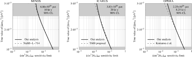
Figure 10: The effective $\sin^{2}2\theta_{13}$ sensitivity limit (as discussed in the main text) at 90% CL as a function of the true value of $\Delta m_{31}^{2}$ for the conventional beam experiments. The exposure is $10\,\mathrm{kt}\,\mathrm{y}$ for MINOS, $20\,\mathrm{kt}\,\mathrm{y}$ for ICARUS and a nominal running time of five years for OPERA, corresponding to an exposure of $8.25\,\mathrm{kt}\,\mathrm{y}$. The dashed gray curves come from the collaborations of the individual experiments and are taken from Ref. [44] for MINOS, Ref. [12] for ICARUS, and Ref. [45] for OPERA. The black curves are obtained for $\sin^{2}2\theta_{23}=1$ and $\Delta m^{2}_{21}=\sin^{2}2\theta_{12}=\delta_{\mathrm{CP}}=0$ for systematics only, i.e., correlations and degeneracies are not included, as for the dashed curves.

Note that the numbers given in Table 5 and the results shown in Figure 10 do not allow a comparison of the different experiment performances, because the reference points used for the calculation of Table 5 are rather different, and so are the integrated luminosities. For a comparison on equal footing we refer to Table 3 and the discussion in Section 5.

Appendix B Simulation of the reactor experiments

For our simulation of the reactor neutrino experiments, we closely follow our previous work in Ref. [20]. For the analyses presented here, we assume a near detector baseline of $L_{\mathrm{ND}}=0.15\,\mathrm{km}$ and we consider two options for the far detector baseline: $L_{\mathrm{FD}}=1.05\,\mathrm{km}$ corresponds to the baseline at the CHOOZ site, whereas a baseline $L_{\mathrm{FD}}=1.7\,\mathrm{km}$ is close to the options considered for several other sites. We always fix the number of reactor neutrino events in the near detector to $2.94\cdot 10^{6}$, which implies that it has the same size as the far detector at $L_{\mathrm{FD}}=1.05\,\mathrm{km}$ with $60\,000$ events (assuming the same efficiencies in both detectors). We allow an uncertainty of the overall reactor neutrino flux normalization of $\sigma_{\mathrm{abs}}=2.5\%$. For the normalization error between the two detectors, we use a typical value of $\sigma_{\mathrm{rel}}=0.6\%$. As shown in Ref. [20], this roughly corresponds to an effective normalization error of $\sigma_{\mathrm{norm}}\simeq 0.8\%$. The total range for the visible energy $E_{\mathrm{vis}}=E_{\bar{\nu}}-\Delta+m_{e}$ (where $\Delta$ is the neutron-proton mass difference, and $m_{e}$ is the electron mass) from 0.5 MeV to 9.2 MeV is divided into 31 bins. Furthermore, we assume a Gaussian energy resolution with $\sigma_{\mathrm{res}}=5\%/\sqrt{E_{\mathrm{vis}}[\mathrm{MeV}]}$. We remark that our results do not change if a smaller bin width is chosen, as it would be allowed by the good energy resolution and the large number of events. Furthermore, we take into account an uncertainty on the energy scale calibration $\sigma_{\mathrm{cal}}=0.5\%$, and an uncertainty on the expected energy spectrum shape $\sigma_{\mathrm{shape}}=2\%$, which we assume to be uncorrelated between the energy bins, but fully correlated between the corresponding bins in near and far detectors (see Ref. [20] for details).

In addition to the analysis as performed in Ref. [20], we have investigated in greater detail the impact of a background for a reactor experiment of the Double-Chooz type. We take into account four different background sources with known shape:

• A background from spallation neutrons coming from muons in the rock close to the detector. This background can be assumed to be flat as a function of energy to a first approximation (see, e.g., Figure 48 of Ref. [10]).

• A background from accidental events. A $\gamma$ from radioactivity is followed by a second random $\gamma$ with more than 6 MeV faking a neutron signal. Those events are important for low energies.

• Two correlated backgrounds from cosmogenic ⁹Li and ⁸He nuclei. Both are created by through-going muons and give $\beta$-spectra with end points of 13.6 and 10.6 MeV, respectively.

In Table 6, we give for each background a realistic estimate [52] for the expected number of events in near and far detectors relative to the number of reactor neutrino events. Since the near detector will have less rock overburden than the far detector, more background events are expected. They are, however, compensated by the much larger number of reactor neutrino events in the near detector. Therefore, we assume to a first approximation the same relative sizes for the backgrounds in near and far detector. In Figure 11, the spectral shape of these backgrounds is shown. We assume that these shapes are exactly known, however, the overall normalization of each of the four background components in the two detectors is allowed to fluctuate independently with an error of $\sigma_{\mathrm{BG}}=50\%$. In addition to these backgrounds with known shape, we include a background from an unidentified source with a bin-to-bin uncorrelated error of 50%. We assume a total number of background events of 0.5% of the reactor signal in both detectors, and a flat energy shape for this background.

Background type	Spectral shape	BG/Reactor events	$\sigma_{\mathrm{BG}}$
Backgrounds with known shape
Spallation neutrons	Flat	0.4%	50%
Accidentals	Low energies	0.2%	50%
Cosmogenic 9Li	$\beta$-spectrum (end point 13.6 MeV)	0.2%	50%
Cosmogenic 8He	$\beta$-spectrum (end point 10.6 MeV)	0.2%	50%
Bin-to-bin correlated BG total:		1.0%
Bin-to-bin uncorrelated background
Unknown source	Flat	0.5%	50%

Table 6: Backgrounds included in our reactor experiment analysis. For each background source, the column “BG/Reactor events” refers to the total number of background events in the energy range between 0.5 and 9.2 $\mathrm{MeV}$ relative to the total number of reactor neutrino events for no oscillations [52]. We assume the same magnitudes of the backgrounds relative to the total events in the near and far detectors. For the backgrounds with known shape, $\sigma_{\mathrm{BG}}$ is the uncertainty of the overall normalization. For the uncorrelated background, $\sigma_{\mathrm{BG}}$ is the error on the number of events in each bin, which is uncorrelated between different bins (31 bins). All backgrounds are uncorrelated between the two detectors.

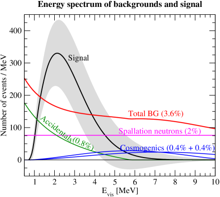
Figure 11: Energy spectrum of the backgrounds from spallation neutrons, accidentals, and cosmogenic ⁹Li and ⁸He. The percentage given for each curve corresponds to the total number of background events relative to the total number of reactor neutrino events for no oscillations. Also shown is the total background spectrum. The curve labeled “signal” corresponds to $N(E_{\mathrm{vis}};\sin^{2}2\theta_{13}=0)-N(E_{\mathrm{vis}};\sin^{2}2\theta_{13}=0.05)$, where $N(E_{\mathrm{vis}};\sin^{2}2\theta_{13})$ is the energy spectrum for given $\sin^{2}2\theta_{13}$. The shaded region is the statistical error band at 1$\sigma$, i.e., $\pm\sqrt{N(E_{\mathrm{vis}};\sin^{2}2\theta_{13}=0)}$. Note that the absolute normalizations of the backgrounds are exaggerated in this figure.

As a general trend, we find that backgrounds with known shape do not significantly affect the sensitivity. This holds independently of the integrated luminosity. Even increasing the numbers given in Table 6 by a factor five does not change the picture. This behavior can be understood in terms of Figure 11, where we show the signal (the spectrum without oscillation minus the spectrum for $\sin^{2}2\theta_{13}=0.05$) and its statistical error compared to the various background spectra. For illustration, background levels significantly larger than in Table 6 are assumed. From this figure, it is obvious that the spectral shape of the signal is very different from that of all of the background components. Already at modest luminosities, such as for Double-Chooz, enough spectral information is available to determine the backgrounds with sufficient accuracy, which means that it is not possible to fake the signal within the statistical error by fluctuations of the background components. In contrast, we find that the bin-to-bin uncorrelated background only plays a minor role for experiments of the size of Double-Chooz, whereas it becomes important for large experiments, such as Reactor-II. In the latter case, a background level of 0.5% with a bin-to-bin uncorrelated error larger than about 20% would significantly affect the sensitivity. We conclude that for large reactor experiments, the shape of the expected background has to be well under control.

In Table 7, we summarize the experimental parameters which we use for the two setups Double-Chooz and Reactor-II in the main text of this study. For the Double-Chooz setup, we stick closely to the configuration discussed in Ref. [23]. We have checked that the effect of the slightly different distances ($1.0\,\mathrm{km}$ and $1.1\,\mathrm{km}$) of the far detector location from the two different reactor cores at the CHOOZ site is very small. Hence it is a good approximation to consider the average baseline of $1.05\,\mathrm{km}$ for both cores. In order to obtain robust results, we include all systematical errors as well as backgrounds.

	Double-Chooz	Reactor-II
Luminosity ${\cal L}$	$288\,\mathrm{t\,GW\,y}$	$8000\,\mathrm{t\,GW\,y}$
Number of events in ND	$2.94\cdot 10^{6}$	$2.94\cdot 10^{6}$
Number of events in FD	$6\cdot 10^{4}$	$6.36\cdot 10^{5}$
Near detector baseline	$0.15\,\mathrm{km}$	$0.15\,\mathrm{km}$
Far detector baseline	$1.05\,\mathrm{km}$	$1.70\,\mathrm{km}$
Energy resolution	$\sigma_{\mathrm{res}}=5\%/\sqrt{E[\mathrm{MeV}]}$
Visible energy range	$0.5-9.2\,\mathrm{MeV}$ (31 bins)
Individual detector normalization	$\sigma_{\mathrm{rel}}=0.6\%$	$\sigma_{\mathrm{rel}}=0.6\%$
Flux normalization	$\sigma_{\mathrm{abs}}=2.5\%$	$\sigma_{\mathrm{abs}}=2.5\%$
Flux shape uncertainty	$\sigma_{\mathrm{shape}}=2\%$	$\sigma_{\mathrm{shape}}=0$
Energy scale error	$\sigma_{\mathrm{cal}}=0.5\%$	$\sigma_{\mathrm{cal}}=0$
Backgrounds included	Yes	No

Table 7: Characteristics of the two reactor experiments Double-Chooz and Reactor-II.

The large reactor experiment Reactor-II corresponds to the same setup as already used in Ref. [20]. It represents an ideal configuration without backgrounds and any systematical errors beyond overall normalization errors. This setup has been chosen to illustrate how an optimal reactor experiment would fit into the general picture of the next ten years of oscillation physics and, to obtain CP-complementary information. Several proposals which are close to our Reactor-II setup are currently discussed [16].

Appendix C The definition of the $\boldsymbol{\sin^{2}2\theta_{13}}$ sensitivity limit

In this appendix, we discuss the definition of the $\sin^{2}2\theta_{13}$ sensitivity limit. Although this definition is very general, we mainly focus on the $\nu_{\mu}\to\nu_{e}$ appearance channel, since one has to deal extensively with parameter correlations and degenerate solutions in this case. Let us first define our $\sin^{2}2\theta_{13}$ sensitivity and then discuss its properties.

Definition 1

We define the $\boldsymbol{\sin^{2}2\theta_{13}}$ sensitivity limit as the largest value of $\sin^{2}2\theta_{13}$, which fits the true value $\sin^{2}2\theta_{13}=0$ at the chosen confidence level. The largest value of $\sin^{2}2\theta_{13}$ is obtained from the projections of all (disconnected) fit manifolds (best-fit manifold and degeneracies) onto the $\sin^{2}2\theta_{13}$-axis.

Since for future experiments no data are available, one has to simulate data by calculating a “reference rate vector” for a fixed set of “true” parameter values. In general, the experiment performance depends on the chosen set of true parameter values, and it is interesting to discuss this dependency in many cases. It is especially relevant for the true values of $\Delta m_{21}^{2}$ and $\Delta m_{31}^{2}$, which we usually choose within their currently allowed ranges. According to Definition 1, we choose the true value $\sin^{2}2\theta_{13}=0$ to calculate the $\sin^{2}2\theta_{13}$ limit, since we are interested in the bound on $\sin^{2}2\theta_{13}$ if no positive signal is observed. Moreover, this choice has the following advantages:

• Since for $\sin^{2}2\theta_{13}=0$ the phase $\delta_{\mathrm{CP}}$ becomes unphysical, the sensitivity limit will be independent of the true value of $\delta_{\mathrm{CP}}$.

• For $\sin^{2}2\theta_{13}=0$, the reference rate vectors for the normal and the inverted mass hierarchies are approximately equal, which implies that the sensitivity limit hardly depends on the true sign of $\Delta m_{31}^{2}$ (see also the discussion related to Figure 12 later).

Once the reference rate vector has been obtained, the fit manifold in the six-dimensional space of the oscillation parameters is given by the requirement $\Delta\chi^{2}\leq\mathrm{CL}$ (e.g., at the 90% confidence level, we have $\mathrm{CL}=2.71$ for 1 d.o.f.). In addition to the allowed region which contains the best-fit point (“best-fit manifold”), one or more disconnected regions (“degenerate solutions”) will exist, and each of them may have a rather complicated shape in the six-dimensional space (“correlations”). The final sensitivity is given by the largest value of $\sin^{2}2\theta_{13}$ which fits $\sin^{2}2\theta_{13}=0$. It is obtained by projecting all these disconnected fit regions onto the $\sin^{2}2\theta_{13}$-axis, where the projection takes into account the correlations. Hence, this procedure provides a straightforward method to take into account correlations and degeneracies. Thus, for the case of the $\nu_{\mu}\to\nu_{e}$ appearance channel, our definition of the $\sin^{2}2\theta_{13}$ sensitivity limit includes the intrinsic structure of Eq. (1). This equation reflects that an appearance experiment is only sensitive to a particular combination of parameters. The projection onto the $\sin^{2}2\theta_{13}$-axis takes into account that all the other parameters can be only measured with a certain accuracy by the experiment itself. Moreover, in complicated cases (e.g., for neutrino factories) local minima may appear in the projection of the $\chi^{2}$-function onto the $\sin^{2}2\theta_{13}$-axis, and the $\chi^{2}$-function can intersect the chosen confidence level multiple times. In this case, we choose by definition the rightmost of these intersections. Hence, the sensitivity limit, as defined above, refers to the potential of an experiment (or combination of experiments) to extract the value of the parameter $\sin^{2}2\theta_{13}$ from Eq. (1) convolved with all the simulation information.

In this study, we compare the $\sin^{2}2\theta_{13}$ sensitivity limit of a given experiment to a so-called $(\sin^{2}2\theta_{13})_{\mathrm{eff}}$ sensitivity limit in some cases. The $(\sin^{2}2\theta_{13})_{\mathrm{eff}}$ sensitivity limit roughly corresponds to the potential of a given experiment to observe a positive signal, which is parameterized by some (unphysical) mixing parameter $(\sin^{2}2\theta_{13})_{\mathrm{eff}}$:

Definition 2

The $\boldsymbol{(\sin^{2}2\theta_{13})_{\mathrm{eff}}}$ sensitivity limit is defined as the sensitivity limit from statistics and systematics only which is computed for $\delta_{\mathrm{CP}}=0$ by fixing all other oscillation parameters to their true values.

In order to illustrate the impact of systematics, correlations, and degeneracies, we often use “bar charts” (see, for example, Figures 3 and 6), where the final $\sin^{2}2\theta_{13}$ sensitivity is obtained by successively switching on systematics, correlations, and degeneracies. In these bar charts, the statistics-only $\sin^{2}2\theta_{13}$ sensitivity (left edge of the bar) is computed for all oscillation parameters fixed and $\delta_{\mathrm{CP}}=0$, the statistics+systematics sensitivity limit corresponds to the $(\sin^{2}2\theta_{13})_{\mathrm{eff}}$ sensitivity limit, the statistics+systematics+correlations limit corresponds to the sensitivity limit for the best-fit manifold only (no degenerate solutions included), and the final sensitivity limit (right edge of the bar) corresponds to Definition 1.

In the following, we illustrate in greater detail how the $\sin^{2}2\theta_{13}$ limit is obtained, how the bar charts are constructed, and how the $\sin^{2}2\theta_{13}$ and $(\sin^{2}2\theta_{13})_{\mathrm{eff}}$ limits are related to each other at the example of the JPARC-SK experiment. We focus mainly on the $\mathrm{sgn}(\Delta m_{31}^{2})$-degeneracy and the correlation between $\theta_{13}$ and $\delta_{\mathrm{CP}}$, which is of particular relevance for the $\nu_{\mu}\to\nu_{e}$ appearance channel at superbeams.

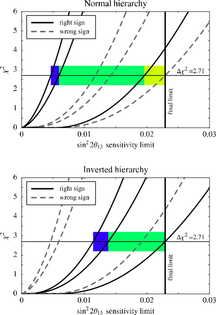
Figure 12: The $\chi^{2}$ as function of $\sin^{2}2\theta_{13}$ for JPARC-SK. For the true values of the oscillation parameters, we choose the current best-fit values from Eq. (3), $\sin^{2}2\theta_{13}=0$, $\delta_{\mathrm{CP}}=0$ (for curves without correlations only), and normal (upper plot) or inverted (lower plot) mass hierarchies. The solid curves in each plot are obtained by fitting with the same mass hierarchy as has been used to calculate the reference rate vector (“right-sign”), whereas for the dashed curves the wrong mass hierarchy has been used (“wrong-sign”). Within each group of solid or dashed curves, the left curve determines the statistics-only limit, the middle curve the statistics+systematics limit, and the right curve the statistics+systematics+correlations limit. Note that the wrong-sign minimum has not exactly the same position in parameter space as the original minimum.

In Figure 12, the $\chi^{2}$ is shown as a function of $\sin^{2}2\theta_{13}$ for the “right-sign” and “wrong-sign” solutions, where in the upper (lower) plot the normal (inverted) hierarchy has been chosen to calculate the reference rate vector. The right-sign solution is obtained by fitting with the same sign of $\Delta m_{31}^{2}$ as the reference rate vector has been calculated with, i.e., the “right” neutrino mass hierarchy is used, whereas the wrong-sign solution is obtained by fitting with the opposite sign of $\Delta m_{31}^{2}$, i.e., the “wrong” mass hierarchy is used. The different curves in each group with the same curve style correspond, from the left to the right, to the statistics-only, statistics+systematics, and statistics+systematics+correlations sensitivity limits, where these limits are obtained from the intersection of the $\chi^{2}$ with the $\Delta\chi^{2}=2.71$ line. The bar charts are constructed from the corresponding curves, as one can easily read off the figure.

Comparing the normal and inverted mass hierarchy plots in Figure 12, one can observe a symmetry between the right- and wrong-sign solutions: The curves for the normal mass hierarchy and $\Delta m_{31}^{2}>0$ (right sign) are very similar to the ones of the inverted mass hierarchy and $\Delta m_{31}^{2}>0$ (wrong sign). This can be understood in terms of the identical appearance rate vectors for the normal and inverted mass hierarchies for the true value of $\sin^{2}2\theta_{13}=0$. However, since the role of the $\Delta m_{31}^{2}>0$ curves is different for the normal and inverted mass hierarchies, i.e., they either correspond to the best-fit manifold (right sign) or the $\mathrm{sgn}(\Delta m_{31}^{2})$-degeneracy (wrong sign), the bar charts are, by definition, very different, since they are originally determined by the best-fit solution. However, one can easily see that the final sensitivity limit does not depend on the mass hierarchy [26]. This property comes from the fact that the degeneracy part does not contribute to the final sensitivity if the best-fit $\sin^{2}2\theta_{13}$ sensitivity is already worse than the degenerate solution sensitivity. Since there is hardly a difference between final sensitivity limits for the different mass hierarchies, we usually show the normal mass hierarchy sensitivity limit. In fact, there is a small difference between the final sensitivity limits for the different mass hierarchies, which mainly comes from the disappearance channels.

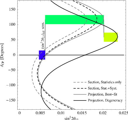
Figure 13: The 90% CL fit manifold (1 d.o.f.) in the $\sin^{2}2\theta_{13}$-$\delta_{\mathrm{CP}}$-plane for JPARC-SK. For the true values of the oscillation parameters, we choose the current best-fit values from Eq. (3) and $\sin^{2}2\theta_{13}=0$. The different curves correspond to various sections (un-displayed oscillation parameters fixed) and projections (minimized over un-displayed oscillation parameters) as described in the plot legend. The bars demonstrate the individual contributions to the final $\sin^{2}2\theta_{13}$ sensitivity limit. Note that for the sgn($\Delta m_{31}^{2}$)-degenerate solution, we only show the final projection.

Let us now illustrate the impact of the correlation between $\sin^{2}2\theta_{13}$ and $\delta_{\mathrm{CP}}$. Therefore, we show in Figure 13 the fit manifold in the $\sin^{2}2\theta_{13}$-$\delta_{\mathrm{CP}}$-plane. The $\sin^{2}2\theta_{13}$ sensitivity limit is again obtained from the projection onto the $\sin^{2}2\theta_{13}$-axis. In Figure 13, the individual contributions to the bar chart are illustrated by showing different sections (un-displayed oscillation parameters fixed, i.e., no correlations) and projections (minimized over un-displayed oscillation parameters, i.e., they include correlations) of the fit manifold. One can see that both edges of the leftmost (blue) bar are computed for $\delta_{\mathrm{CP}}=0$. This illustrates that if $\delta_{\mathrm{CP}}$ and all the other oscillation parameters except $\sin^{2}2\theta_{13}$ are fixed at the true values, much stronger bounds on $\sin^{2}2\theta_{13}$ can be obtained, corresponding to the $(\sin^{2}2\theta_{13})_{\mathrm{eff}}$ limit. The limit gets considerably weaker if the $\chi^{2}$-function is minimized over $\delta_{\mathrm{CP}}$, as well as all oscillation parameters which are not shown, which leads to the “correlation bar”. In fact, from Figure 13, one can see that the largest part of the correlation bar comes from the correlation with $\delta_{\mathrm{CP}}$ [53], and only the small difference between the dark dashed and the light solid curves comes from the correlation with the other oscillation parameters. The final sensitivity limit is then obtained as the maximum value of $\sin^{2}2\theta_{13}$ which fits $\sin^{2}2\theta_{13}=0$ including all degenerate solutions.

References

- [1] Y. Fukuda et al. (Super-Kamiokande), Phys. Rev. Lett. 81, 1562 (1998), hep-ex/9807003; Phys. Rev. Lett. 82, 2644 (1999), hep-ex/9812014.
- [2] Y. Hayato (Super-Kamiokande) Talk at the HEP2003 conference (Aachen, Germany, 2003), http://eps2003.physik.rwth-aachen.de.
- [3] M. Ambrosio et al. (MACRO), Phys. Lett. B566, 35 (2003), hep-ex/0304037.
- [4] M. H. Ahn et al. (K2K), Phys. Rev. Lett. 90, 041801 (2003), hep-ex/0212007.
- [5] B. T. Cleveland et al., Astrophys. J. 496, 505 (1998); J. N. Abdurashitov et al. (SAGE), J. Exp. Theor. Phys. 95, 181 (2002); W. Hampel et al. (GALLEX), Phys. Lett. B447, 127 (1999); M. Altmann et al. (GNO), Phys. Lett. B490, 16 (2000), hep-ex/0006034; S. Fukuda et al. (Super-Kamiokande), Phys. Lett. B539, 179 (2002), hep-ex/0205075; Q. R. Ahmad et al. (SNO), Phys. Rev. Lett. 89, 011301 (2002), nucl-ex/0204008.
- [6] S. N. Ahmed et al. (SNO) (2003), nucl-ex/0309004.
- [7] K. Eguchi et al. (KamLAND), Phys. Rev. Lett. 90, 021802 (2003), hep-ex/0212021.
- [8] L. Wolfenstein, Phys. Rev. D17, 2369 (1978); S. P. Mikheev and A. Y. Smirnov, Sov. J. Nucl. Phys. 42, 913 (1985).
- [9] M. Apollonio et al. (CHOOZ), Phys. Lett. B466, 415 (1999), hep-ex/9907037.
- [10] M. Apollonio et al. (CHOOZ), Eur. Phys. J. C27, 331 (2003), hep-ex/0301017.
- [11] E. Ables et al. (MINOS) FERMILAB-PROPOSAL-P-875.
- [12] P. Aprili et al. (ICARUS) CERN-SPSC-2002-027.
- [13] D. Duchesneau (OPERA), eConf C0209101, TH09 (2002), hep-ex/0209082.
- [14] Y. Itow et al., Nucl. Phys. Proc. Suppl. 111, 146 (2001), hep-ex/0106019.
- [15] D. Ayres et al. (2002), hep-ex/0210005.
- [16] K. Anderson et al. (2004), hep-ex/0402041.
- [17] F. Boehm et al., Phys. Rev. D64, 112001 (2001), hep-ex/0107009.
- [18] L. A. Mikaelyan and V. V. Sinev, Phys. Atom. Nucl. 63, 1002 (2000), hep-ex/9908047; V. Martemyanov, L. Mikaelyan, V. Sinev, V. Kopeikin, and Y. Kozlov, Phys. Atom. Nucl. 66, 1934 (2003), hep-ex/0211070.
- [19] H. Minakata, H. Sugiyama, O. Yasuda, K. Inoue, and F. Suekane, Phys. Rev. D68, 033017 (2003), hep-ph/0211111.
- [20] P. Huber, M. Lindner, T. Schwetz, and W. Winter, Nucl. Phys. B665, 487 (2003), hep-ph/0303232.
- [21] M. H. Shaevitz and J. M. Link (2003), hep-ex/0306031.
- [22] K. Heeger, Measuring theta13 with reactor neutrinos: Initiatives in the US, Talk given at NOON 2004, available at http://www-sk.icrr.u-tokyo.ac.jp/noon2004/.
- [23] Double-Chooz Letter of Intent, in preparation.
- [24] M. Shaevitz, Talk given at the APS Neutrino Study, working group meeting, Feb. (2004), http://apsreactor.uchicago.edu/meetings/chicago/shaevitz.pdf.
- [25] D. Beavis et al., Proposal of BNL AGS E-889, Tech. Rep., BNL (1995).
- [26] P. Huber, M. Lindner, and W. Winter, Nucl. Phys. B654, 3 (2003), hep-ph/0211300.
- [27] P. Huber, M. Lindner, and W. Winter, Nucl. Phys. B645, 3 (2002), hep-ph/0204352.
- [28] NuMI off-axis proposal, in preparation; see http://www-off-axis.fnal.gov/.
- [29] V. Barger, D. Marfatia, and K. Whisnant, Phys. Lett. B560, 75 (2003), hep-ph/0210428.
- [30] H. Minakata, H. Nunokawa, and S. J. Parke, Phys. Rev. D68, 013010 (2003), hep-ph/0301210.
- [31] H. Minakata and H. Sugiyama, Phys. Lett. B580, 216 (2004), hep-ph/0309323.
- [32] K. Hagiwara et al. (Particle Data Group), Phys. Rev. D66, 010001 (2002).
- [33] R. J. Geller and T. Hara, Phys. Rev. Lett. 49, 98 (2001), hep-ph/0111342; T. Ohlsson and W. Winter, Phys. Rev. D68, 073007 (2003), hep-ph/0307178; S. V. Panasyuk, Rem (reference earth model) web page (2000), http://cfauvcs5.harvard.edu/lana/rem/index.htm.
- [34] P. Huber, M. Lindner, and W. Winter, GLoBES (Global Long Baseline Experiment Simulator), http://www.ph.tum.de/∼globes.
- [35] M. Freund, P. Huber, and M. Lindner, Nucl. Phys. B615, 331 (2001), hep-ph/0105071; M. Freund, Phys. Rev. D64, 053003 (2001), hep-ph/0103300; A. Cervera et al., Nucl. Phys. B579, 17 (2000), hep-ph/0002108.
- [36] E. K. Akhmedov, R. Johansson, M. Lindner, T. Ohlsson, and T. Schwetz (2004), hep-ph/0402175.
- [37] J. Burguet-Castell, M. B. Gavela, J. J. Gomez-Cadenas, P. Hernandez, and O. Mena, Nucl. Phys. B608, 301 (2001), hep-ph/0103258.
- [38] H. Minakata and H. Nunokawa, JHEP 10, 001 (2001), hep-ph/0108085.
- [39] G. L. Fogli and E. Lisi, Phys. Rev. D54, 3667 (1996), hep-ph/9604415.
- [40] V. Barger, D. Marfatia, and K. Whisnant, Phys. Rev. D65, 073023 (2002), hep-ph/0112119.
- [41] G. L. Fogli, E. Lisi, A. Marrone, and D. Montanino, Phys. Rev. D67, 093006 (2003), hep-ph/0303064; G. L. Fogli et al., Phys. Rev. D69, 017301 (2004), hep-ph/0308055.
- [42] M. Maltoni, T. Schwetz, M. A. Tortola, and J. W. F. Valle, Phys. Rev. D68, 113010 (2003), hep-ph/0309130.
- [43] M. C. Gonzalez-Garcia and C. Pea-Garay, Phys. Lett. B527, 199 (2002), hep-ph/0111432; V. D. Barger, D. Marfatia, and B. P. Wood, Phys. Lett. B498, 53 (2001), hep-ph/0011251.
- [44] M. Diwan et al. (MINOS), A study of sensitivity in MINOS, Tech. Rep. NuMI-L-714 (2001).
- [45] M. Komatsu, P. Migliozzi, and F. Terranova, J. Phys. G29, 443 (2003), hep-ph/0210043.
- [46] P. Migliozzi and F. Terranova, Phys. Lett. B563, 73 (2003), hep-ph/0302274.
- [47] V. D. Barger et al., Phys. Rev. D65, 053016 (2002), hep-ph/0110393.
- [48] W. Winter Phys. Rev. D70, 033006 (2003), hep-ph/0310307.
- [49] Y. F. Wang, K. Whisnant, Z.-h. Xiong, J. M. Yang, and B.-L. Young (VLBL Study Group H2B-4), Phys. Rev. D65, 073021 (2002), hep-ph/0111317; M. Apollonio et al. (2002), hep-ph/0210192; K. Whisnant, J. M. Yang, and B.-L. Young, Phys. Rev. D67, 013004 (2003), hep-ph/0208193; V. Barger, D. Marfatia, and K. Whisnant, Phys. Rev. D66, 053007 (2002), hep-ph/0206038; J. Bouchez, M. Lindroos, and M. Mezzetto (2003), hep-ex/0310059; J. Burguet-Castell, M. B. Gavela, J. J. Gomez-Cadenas, P. Hernandez, and O. Mena, Nucl. Phys. B646, 301 (2002), hep-ph/0207080; A. Donini, D. Meloni, and P. Migliozzi, Nucl. Phys. B646, 321 (2002), hep-ph/0206034; P. Zucchelli, Phys. Lett. B532, 166 (2002); J. Burguet-Castell, D. Casper, J. J. Gomez-Cadenas, P. Hernandez, and F. Sanchez (2003), hep-ph/0312068; P. Huber and W. Winter, Phys. Rev. D68, 037301 (2003), hep-ph/0301257; D. Autiero et al. (2003), hep-ph/0305185; A. Asratyan et al., Science 124, 103 (2003), hep-ex/0303023; W. Winter (2003), hep-ph/0308227.
- [50] M. Goodman, private communication; M. D. Messier, private communication.
- [51] CNGS, http://proj-cngs.web.cern.ch/proj-cngs/Menu/CNGS.htm.
- [52] H. de Kerret, private communication.
- [53] T. Kajita, H. Minakata, and H. Nunokawa, Phys. Lett. B528, 245 (2002), hep-ph/0112345.