Quark Propagation in the Quark-Gluon Plasma

Abstract

It has recently been suggested that the quark-gluon plasma formed in heavy-ion collisions behaves as a nearly ideal fluid. That behavior may be understood if the quark and antiquark mean-free- paths are very small in the system, leading to a “sticky molasses” description of the plasma, as advocated by the Stony Brook group. This behavior may be traced to the fact that there are relatively low-energy $q\overline{q}$ resonance states in the plasma leading to very large scattering lengths for the quarks. These resonances have been found in lattice simulation of QCD using the maximum entropy method (MEM). We have used a chiral quark model, which provides a simple representation of effects due to instanton dynamics, to study the resonances obtained using the MEM scheme. In the present work we use our model to study the optical potential of a quark in the quark-gluon plasma and calculate the quark mean-free-path. Our results represent a specific example of the dynamics of the plasma as described by the Stony Brook group.

I INTRODUCTION

The description of the quark-gluon plasma in terms of hydrodynamics has been advocated by the Stony Brook group [ 1-3 ]. That description appears to be in accord with the experimental data. In such a description the motion of the quarks is characterized by an extremely short mean-free-path. The origin of that behavior is thought to be due to the relatively low-energy resonances in the $q\overline{q}$ system leading to very large scattering lengths. These resonances have been found in lattice studies of QCD which make use of the maximum entropy method (MEM) [ 4-9 ]. Similar resonances are found in the scalar, pseudoscalar, vector and axial-vector $q\overline{q}$ channels [ 10 ]. Recently, an extensive exploration of charmonium studies in the confined and deconfined regions using lattice methods has been reported in Ref. [11]. In that work results are given for the dependence of the resonance excitation on the total momentum of the $q\overline{q}$ pair. We have studied that dependence for light quark systems in Ref.[12] and have found similar behavior to that reported in Ref. [11]. (We will make use of the results presented in Ref. [12] in the present work in which we calculate the imaginary part of the optical potential and the mean-free-path for a quark in the quark-gluon plasma.) We use a chiral model with rather large momentum cutoff. That model is meant to provide an approximate description of the instanton dynamics advocated by the Stony Brook group [1-3]. Earlier work using our model may be found in Refs. [13-15].

In our studies of meson spectra at $T=0$ and at $T<T_{c}$ we have made use of the Nambu–Jona-Lasinio (NJL) model. The Lagrangian of the generalized NJL model we have used in our studies is

$$\mathcal{L} = \overline{q}(i\hbox to0.0pt{\hbox to5.1773pt{\hfil/\hfil}\hss}\gamma-m^{0})q+\frac{\overline{G}_{S}}{2}\sum_{i=0}^{8}[(\overline{q}\lambda^{i}q)^{2}+(\overline{q}i\gamma_{5}\lambda^{i}q)^{2}]$$

$$- \frac{\overline{G}_{V}}{2}\sum_{i=0}^{8}[(\overline{q}\lambda^{i}\gamma_{\mu}q)^{2}+(\overline{q}\lambda^{i}\gamma_{5}\gamma_{\mu}q)^{2}]$$

$$+ \frac{G_{D}}{2}\{\det[\overline{q}(1+\lambda_{5})q]+\det[\overline{q}(1-\lambda_{5})q]\}+\mathcal{L}_{conf}$$

Here, $m^{0}$ is a current quark mass matrix, $m^{0}=diag(m_{u}^{0},m_{d}^{0},m_{s}^{0})$. The $\lambda_{i}$ are the Gell-Mann (flavor) matrices and $\lambda^{0}=\sqrt{2/3}\mathbf{1}$, with $\mathbf{1}$ being the unit matrix. The fourth term is the ’t Hooft interaction and $\mathcal{L}_{conf}$ represents the model of confinement used in our studies of meson properties.

In the study of hadronic current correlators [13-15] it is important to use a model which respects chiral symmetry when $m^{0}=0$. Therefore, we make use of the Lagrangian of Eq. (1.1), while neglecting the ’t Hooft interaction and $\mathcal{L}_{conf}$. In order to make contact with the results of lattice simulations we use the model with the number of flavors $N_{f}=1$. Therefore, the $\lambda^{i}$ matrices in Eq. (1.1) may be replaced by unity. We then use

$$\mathcal{L} = \overline{q}(i\hbox to0.0pt{\hbox to5.1773pt{\hfil/\hfil}\hss}\gamma-m^{0})q+\frac{G_{S}}{2}[(\overline{q}q)^{2}+(\overline{q}i\gamma_{5}q)^{2}]$$

$$- \frac{G_{V}}{2}[(\overline{q}\gamma_{\mu}q)^{2}+(\overline{q}\gamma_{5}\gamma_{\mu}q)^{2}]$$

in order to calculate the hadronic current correlation functions. Thus, there are essentially three parameters to consider, $G_{S}$, $G_{V}$ and a Gaussian cutoff parameter $\alpha$, which restricts the momentum integrals through a factor $\exp[-\overrightarrow{k}^{2}/\alpha^{2}]$. As suggested by the Stony Brook group, we consider the NJL model and the associated chiral Lagrangian of Eq. (1.2) as providing a simplified representation of the instanton dynamics important for the problems considered in this work. Since the results obtained for the hadronic current correlation functions are similar in the scalar, pseudoscalar, vector and axial-vector channels, we carry out our calculations for the scalar $q\overline{q}$ states and multiple our results for the optical potential by 4. The parameters G and $\alpha$ were fixed in our earlier studies [12]. We take G =1.0 GeV^-2 and $\alpha$ = 4.4 GeV. These values provide good fits [12] to the hadronic current correlation functions found in the lattice studies [10]. In order to calculate the optical potential for a quark we consider the quark moving in an antiquark distribution characterized by a temperature-dependent occupation factor $n(\overrightarrow{p_{1}})$ which depends upon the chemical potential $\mu$. The energy of a quark is given by $E(\overrightarrow{p})=[\overrightarrow{p}^{2}+m^{2}]^{1/2}$. We follow the work of Shuryak [1], for example, and put $m$ = 1 GeV. In Shuryak’s work this mass is not the current quark mass, but is called the “chiral mass”. (We would prefer to call the 1 GeV mass, the “thermal mass”, however, the terminology used is not important for this work.) The quark thermal mass is given in Ref. [16], with $C_{F}=4/3$, as

$$m^{2}=\frac{1}{8}g^{2}C_{F}(T^{2}+\frac{\mu^{2}}{\pi^{2}}),$$ (1.3)

for the case of a finite chemical potential. The thermal gluon mass is

$$m_{g}^{2}=\frac{1}{6}g^{2}T^{2}(C_{A}+\frac{1}{2}N_{f}).$$ (1.4)

(The relation between thermal masses in QED and QCD is given on p.146 of Ref. [ 16 ].) In studies of baryon matter, the chemical potentials used are often about 300 MeV or less. However, once we introduce a thermal mass of about 1 GeV, we need to determine the chemical potential for the quarks. In this work we will consider a chemical potential of about 1 GeV, although the calculations are easily made for other values. Once we put $m$ = 1 GeV, the chemical potential is the only parameter which is varied in our study. The organization of our work is as follows. In Section II we discuss the calculation of the imaginary part of the quark optical potential and the quark mean-free-path. Section III contains some further discussion and conclusions. (Appendixes A and B provide a description of the calculation of correlators in our model. That description is readily taken over to obtain a representation of the $q\overline{q}$ scattering matrix. The calculation of the vacuum polarization function $J(P^{0},\overrightarrow{P}$) which appears in Section II is described in the appendices.)

II calculation of the quark optical potential

It is useful to contrast the calculation of the quark optical potential with the calculation of the nucleon optical potential that is to be used in the Dirac equation. The latter calculation is discussed in detail in Ref. [17]. In that calculation of the nucleon-nucleus potential one calculates the T-matrix for nucleon-nucleon scattering using the one-boson-exchange (OBE) model. In that case the mesons of the OBE model undergo t-channel and u-channel exchange between the nucleons. The result is that the imaginary part of the optical potential has a magnitude of about 10 MeV [17]. That in turn leads to a mean-free-path of about 10 fm for a 500 MeV nucleon. Many years ago, the relatively large value for the nucleon mean-free-path lead to the characterization of the optical model for nucleon-nucleus scattering as the “cloudy crystal ball” model. When we study quark propagation in the quark-gluon plasma we may consider a similar calculation of the optical potential at finite temperature. In the case of the quark-antiquark interaction the T matrix is dominated by s-channel resonances of the type found in the MEM studies. As we will see, the interaction in this case is quite strong, leading to a small mean-free-path. The resulting model is called the “sticky molasses” model [1-3] as opposed to the “cloudy crystal ball” model used to describe nucleon-nucleus scattering. We now consider the potential seen by a quark of momentum $\overrightarrow{p_{2}}$ and average over the quark spin $s_{2}$. (We will consider quarks of a single flavor, since that was done in the MEM studies that we have used to fix the parameters of our model.) In Ref. [17] the relativistic optical potential was denoted as $\Sigma(\overrightarrow{p},s)$ and, for this work, we consider

$$\Sigma^{++}(\overrightarrow{p_{2}})=\frac{1}{2}\sum_{s_{2}}\overline{u}(\overrightarrow{p_{2}},s_{2})\Sigma(\overrightarrow{p_{2}},s_{2})u(\overrightarrow{p_{2}},s_{2}).$$ (2.1)

It is useful to introduce [14]

$$U(\overrightarrow{p_{2}})=N\sqrt{\frac{m}{E(\overrightarrow{p_{2}})}}\Sigma^{++}(\overrightarrow{p_{2}})\sqrt{\frac{m}{E(\overrightarrow{p_{2}})}}.$$ (2.2)

Here the factor of N = 4 takes into account the sum of the interactions in the scalar, pseudoscalar, vector and axial-vector channels which are taken to be equal for the purposes of this work. The approximate equality of the interactions in these channels may be seen in Ref. [10]. (Note that values of $U(\overrightarrow{p})$ are given in Ref. [17] for the case of nucleon-nucleus scattering.)

If $p_{1}$ is the momentum of the antiquark in the medium, we may introduce the four-vector

$$P^{\mu}=(p_{1}+p_{2})^{\mu}.$$ (2.3)

Now

$$P^{2} = P_{0}^{2}-\overrightarrow{P}^{2}$$ (2.4)

$$= (E(\overrightarrow{p_{1}})+E(\overrightarrow{p_{2}}))^{2}-(\overrightarrow{p_{1}}^{2}+\overrightarrow{p_{2}}^{2}+2p_{1}p_{2}\cos\theta).$$ (2.5)

Here, we take $\overrightarrow{p_{2}}$ along the $z$ axis. We define

$$t(\overrightarrow{p_{1}},\overrightarrow{p_{2}})=\frac{1}{\pi P^{2}}\left[\frac{G}{1-GJ(\overrightarrow{p_{1}},\overrightarrow{p_{2}})}\right],$$ (2.6)

where $J(\overrightarrow{p_{1}},\overrightarrow{p_{2}})$ is the $q\overline{q}$ vacuum polarization function defined in Appendix B. (We remark that we may also use the notation $t(P^{2},p_{2})$ for the quantity defined in Eq. (2.6).)

It is also useful to introduce the occupation factor $n(\overrightarrow{p_{1}})$:

$$n(\overrightarrow{p_{1}})=\frac{1}{\exp\beta[E(\overrightarrow{p_{1}})-\mu]+1},$$ (2.7)

with $\beta=1/T$ and $E(\overrightarrow{p_{1}})=\left[\overrightarrow{p_{1}}^{2}+m^{2}\right]^{1/2}$. We recall

$$\sum_{s_{2}}u(p_{2},s_{2})\overline{u}(p_{2},s_{2})=\left(\frac{\hbox to0.0pt{\hbox to5.03125pt{\hfil/\hfil}\hss}p_{2}+m}{2m}\right),$$ (2.8)

$$\sum_{s_{1}}v(p_{1},s_{1})\overline{v}(p_{1},s_{1})=\left(\frac{\hbox to0.0pt{\hbox to5.03125pt{\hfil/\hfil}\hss}p_{1}-m}{2m}\right),$$ (2.9)

and note that

$$\mbox{Tr}\left(\frac{\hbox to0.0pt{\hbox to5.03125pt{\hfil/\hfil}\hss}p_{2}+m}{2m}\right)\left(\frac{\hbox to0.0pt{\hbox to5.03125pt{\hfil/\hfil}\hss}p_{1}-m}{2m}\right)=\left[\frac{(E_{1}E_{2}-\overrightarrow{p_{1}}\cdot\overrightarrow{p_{2}})-m^{2}}{m^{2}}\right].$$ (2.10)

Thus,

$$\mbox{Im}\Sigma^{++}(p_{2})=-\frac{1}{2}\int\frac{d\overrightarrow{p_{1}}}{(2\pi)^{3}}\frac{m}{E(\overrightarrow{p_{1}})}\mbox{Im}\left[\frac{G}{1-GJ(\overrightarrow{p_{1}},\overrightarrow{p_{2}})}\right]$$ (2.11)

$$\times\left[\frac{E_{1}E_{2}-\overrightarrow{p_{1}}\cdot\overrightarrow{p_{2}}-m^{2}}{m^{2}}\right]n(\overrightarrow{p_{1}}),$$

and

$$U(\overrightarrow{p_{2}})=-\frac{N}{2}\frac{m}{E(\overrightarrow{p_{2}})}\int\frac{d\overrightarrow{p_{1}}}{(2\pi)^{3}}\frac{m}{E(\overrightarrow{p_{1}})}\pi P^{2}t(\overrightarrow{p_{1}},\overrightarrow{p_{2}})$$ (2.12)

$$\times\left[\frac{E_{1}E_{2}-\overrightarrow{p_{1}}\cdot\overrightarrow{p_{2}}-m^{2}}{m^{2}}\right]n(\overrightarrow{p_{1}}).$$

Here $E_{1}=E(\overrightarrow{p_{1}})$, $E_{2}=E(\overrightarrow{p_{2}})$ and we have made use of Eqs. (2.2) and (2.6). Values of $t(P^{2},p_{2})$ are shown in Fig. 1 for values of $|\overrightarrow{p_{2}}|$ ranging from 0.01 GeV to 0.31 GeV. In Fig. 2 we show the values of $n(\overrightarrow{p_{1}})$ for the three values of $\mu$ considered here and in Fig. 3 we present values of Im$U(\overrightarrow{p_{2}})$ for those values of $\mu$. In Fig. 4 we show the values for the mean-free-path

$$\lambda=\frac{|\overrightarrow{p_{2}}|}{m}\frac{1}{\mbox{Im}U(\overrightarrow{p_{2}})}.$$ (2.13)

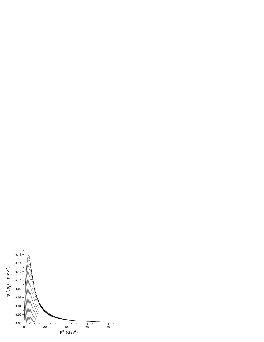
Figure 1: Values of $t(P^{2},p_{2})$ are shown for various values of the quark momentum $|\vec{p}_{2}|$. Starting with the uppermost curve, the $|\vec{p}_{2}|$ values in GeV units are 0.01, 0.03, 0.05, 0.07, 0.09, 0.11, 0.13, 0.15, 0.17, 0.19, 0.21, 0.23, 0.25, 0.27, 0.29 and 0.31. (For large $P^{2}$, we have $t(P^{2},p_{2})\simeq(1/\pi P^{2})G$.) Here $P^{2}=(p_{1}+p_{2})^{2}$, where $p_{1}$ is the antiquark momentum.

Figure 2: Values of $n(p_{1})$ are shown for $\mu=1.1$ GeV (dotted curve), $\mu=1.3$ GeV (dashed curve) and $\mu=1.5$ GeV (solid curve). Here $T=1.5\,T_{c}$ with $T_{c}=270$ MeV.

Figure 3: The imaginary part of the quark optical potential is shown for $\mu=1.1$ GeV (dotted curve), $\mu=1.3$ GeV (dashed curve) and $\mu=1.5$ GeV (solid curve). (We recall that the nucleon-nucleus imaginary optical potential is about 0.01 GeV in magnitude [17].)

Figure 4: Values of $\lambda(p_{2})$ are shown for $\mu=1.1$ GeV (dotted curve), $\mu=1.3$ GeV (dashed curve) and $\mu=1.5$ GeV (solid curve).

III discussion

Information is available concerning the baryon chemical potential. That chemical potential is parameterized in Ref. [18] as

$$\mu_{B}=\frac{1270\,\mbox{MeV}}{(1+\frac{\sqrt{S_{NN}}}{4.3})},$$ (3.1)

and varies strongly with $\sqrt{S_{NN}}$, which is in GeV units in Eq. (3.1). For $\sqrt{S_{NN}}$ = 200 GeV, we have $\mu_{B}$ = 26.7 MeV.

Of particular significance for our results is the choice of the chemical potential for the quarks. We have taken $\mu\sim$ 1 GeV. In the case of the quarks, the choice of $\mu\simeq$ 1 GeV leads to small mean-free-paths consistent with the suggestion of Shuryak that the resonances seen in the MEM analysis of the lattice results are responsible for the small mean-free-paths of the “sticky molasses” model.

We remark that in nuclear matter the baryon density is 0.17 fm^-3 or 0.51 quarks/fm³ if we consider the nucleon to be composed of three quarks. For the values of $n(\overrightarrow{p_{1}})$ shown in Fig. 2 for the case $\mu$ = 1.3 GeV, we may calculate the density of antiquarks to be 5.91 fm^-3, so that the density of quarks and antiquarks is about 12 fm^-3 in our model. We remark that the energy density at RHIC for $\sqrt{S_{NN}}$ = 200 GeV is 4.1 GeV/fm³ [18], which is about 26 times the energy density of nuclear matter, which is approximately 0.16 GeV/fm³.

In this work we have attempted to provide a quantitative analysis of the suggestion [1] that the large $q\overline{q}$ resonant scattering cross sections are responsible for the small quark mean-free-paths, with the associated relevance of the hydrodynamic description of the system that is created in high-energy nucleus-nucleus collisions. We have considered the interaction in the scalar, pseudoscalar, vector and axial-vector channels of the $q\overline{q}$ system. It is possible that there are important resonances of $qq$ character, as well as the $q\overline{q}$ resonances considered here. Such $qq$ states are depicted in Fig. 8a of Ref. [1]. It would be of interest to see if such states are found in lattice studies using the MEM scheme.

Appendix A

For ease of reference, we present a discussion of our calculation of hadronic current correlators taken from Ref. [ 15 ]. The procedure we adopt is based upon the real-time finite-temperature formalism, in which the imaginary part of the polarization function may be calculated. Then, the real part of the function is obtained using a dispersion relation. The result we need for this work has been already given in the work of Kobes and Semenoff [ 19 ]. (In Ref. [ 19 ] the quark momentum is $k^{\mu}$ and the antiquark momentum is $k^{\mu}-P^{\mu}$. We will adopt that notation in this section for ease of reference to the results presented in Ref. [ 19 ].) With reference to Eq. (5.4) of Ref. [ 19 ], we write the imaginary part of the scalar polarization function as

$$\mbox{Im}\,J_{S}(\textit{P}\,{}^{2},T)=\frac{1}{2}N_{c}\beta_{S}\,\epsilon(\textit{P}\,{}^{0})\!\int\!\!\frac{d^{3}\!{k}}{(2\pi)^{3}}\,e^{-\vec{k}\,{}^{2}/\alpha^{2}}\left(\frac{2\pi}{2E_{1}(k)2E_{2}(k)}\right)$$ (A1)

$$\times\{[1-n_{1}(k)-n_{2}(k)]\delta(\textit{P}\,{}^{0}-E_{1}(k)-E_{2}(k))$$

$$-[n_{1}(k)-n_{2}(k)]\delta(\textit{P}\,{}^{0}+E_{1}(k)-E_{2}(k))$$

$$-[n_{2}(k)-n_{1}(k)]\delta(\textit{P}\,{}^{0}-E_{1}(k)+E_{2}(k))$$

$$-[1-n_{1}(k)-n_{2}(k)]\delta(\textit{P}\,{}^{0}+E_{1}(k)+E_{2}(k))\}\,.$$

Here, $E_{1}(k)=[\,\vec{k}\,{}^{2}+m_{1}^{2}(T)\,]^{1/2}$. Relative to Eq. (5.4) of Ref. [ 19 ], we have changed the sign, removed a factor of $g^{2}$ and have included a statistical factor of $N_{c}$. In addition, we have included a Gaussian regulator, $\exp[\,-\vec{k}\,{}^{2}/\alpha^{2}\,]$. The value $\alpha=0.605$ GeV was used in our applications of the NJL model in the calculation of meson properties at $T=0$. We also note that

$$n_{1}(k)=\frac{1}{e^{\,\beta E_{1}(k)}+1}\,,$$ (A2)

and

$$n_{2}(k)=\frac{1}{e^{\,\beta E_{2}(k)}+1}\,.$$ (A3)

For the calculation of the imaginary part of the polarization function, we may put $k^{2}=m_{1}^{2}(T)$ and $(k-P)^{2}=m_{2}^{2}(T)$, since in that calculation the quark and antiquark are on-mass-shell. In Eq. (A1) the factor $\beta_{S}$ arises from a trace involving Dirac matrices, such that

$$\beta_{S} = -\mbox{Tr}[\,(\hbox to0.0pt{\hbox to5.52084pt{\hfil/\hfil}\hss}k+m_{1})(\hbox to0.0pt{\hbox to5.52084pt{\hfil/\hfil}\hss}k-\hbox to0.0pt{\hbox to7.80904pt{\hfil/\hfil}\hss}P+m_{2})\,]$$ (A4)

$$= 2P^{2}-2(m_{1}+m_{2})^{2}\,,$$ (A5)

where $m_{1}$ and $m_{2}$ depend upon temperature. In the frame where $\vec{P}=0$, and in the case $m_{1}=m_{2}$, we have $\beta_{S}=2P_{0}^{2}(1-{4m^{2}}/{P_{0}^{2}})$. For the scalar case, with $m_{1}=m_{2}$, we find

$$\mbox{Im}\,J_{S}(P^{2},T)=\frac{N_{c}P_{0}^{2}}{8\pi}\left(1-\frac{4m^{2}(T)}{P_{0}^{2}}\right)^{3/2}e^{-\vec{k}\,{}^{2}/\alpha^{2}}[\,1-2n_{1}(k)\,]\,,$$ (A6)

where

$$\vec{k}\,{}^{2}=\frac{P_{0}^{2}}{4}-m^{2}(T)\,.$$ (A7)

For pseudoscalar mesons, we replace $\beta_{S}$ by

$$\beta_{P} = -\mbox{Tr}[\,i\gamma_{5}(\hbox to0.0pt{\hbox to5.52084pt{\hfil/\hfil}\hss}k+m_{1})i\gamma_{5}(\hbox to0.0pt{\hbox to5.52084pt{\hfil/\hfil}\hss}k-\hbox to0.0pt{\hbox to7.80904pt{\hfil/\hfil}\hss}P+m_{2})\,]$$ (A8)

$$= 2P^{2}-2(m_{1}-m_{2})^{2}\,,$$ (A9)

which for $m_{1}=m_{2}$ is $\beta_{P}=2P_{0}^{2}$ in the frame where $\vec{P}=0$. We find, for the $\pi$ mesons,

$$\mbox{Im}\,J_{P}(P^{2},T)=\frac{N_{c}P_{0}^{2}}{8\pi}\left(1-\frac{4m^{2}(T)}{P_{0}^{2}}\right)^{1/2}e^{-\vec{k}\,{}^{2}/\alpha^{2}}[\,1-2n_{1}(k)\,]\,,$$ (A10)

where $\vec{k}\,{}^{2}={P_{0}^{2}}/4-m_{u}^{2}(T)$, as above. Thus, we see that the phase space factor has an exponent of 1/2 corresponding to a s-wave amplitude. For the scalars, the exponent of the phase-space factor is 3/2, as seen in Eq. (A6).

For a study of vector mesons we consider

$$\beta_{\mu\nu}^{V}=\mbox{Tr}[\,\gamma_{\mu}(\hbox to0.0pt{\hbox to5.52084pt{\hfil/\hfil}\hss}k+m_{1})\gamma_{\nu}(\hbox to0.0pt{\hbox to5.52084pt{\hfil/\hfil}\hss}k-\hbox to0.0pt{\hbox to7.80904pt{\hfil/\hfil}\hss}P+m_{2})\,]\,,$$ (A11)

and calculate

$$g^{\mu\nu}\beta_{\mu\nu}^{V}=4[\,P^{2}-m_{1}^{2}-m_{2}^{2}+4m_{1}m_{2}\,]\,,$$ (A12)

which, in the equal-mass case, is equal to $4P_{0}^{2}+8m^{2}(T)$, when $\vec{P}=0$. This result is needed when we calculate the correlator of vector currents. Note that, for the elevated temperatures considered in this work, $m_{u}(T)=m_{d}(T)$ is quite small, so that $4P_{0}^{2}+8m_{u}^{2}(T)$ can be approximated by $4P_{0}^{2}$, when we consider the vector current correlation functions. In that case, we have

$$\mbox{Im}\,J_{V}(P^{2},T)\simeq\frac{2}{3}\mbox{Im}\,J_{P}(P^{2},T)\,.$$ (A13)

At this point it is useful to define functions that do not contain that Gaussian regulator:

$$\mbox{Im}\,\tilde{J}_{P}(P^{2},T)=\frac{N_{c}P_{0}^{2}}{8\pi}\left(1-\frac{4m^{2}(T)}{P_{0}^{2}}\right)^{1/2}[\,1-2n_{1}(k)\,]\,,$$ (A14)

and

$$\mbox{Im}\,\tilde{J}_{V}(P^{2},T)=\frac{2}{3}\frac{N_{c}P_{0}^{2}}{8\pi}\left(1-\frac{4m^{2}(T)}{P_{0}^{2}}\right)^{1/2}[\,1-2n_{1}(k)\,]\,,$$ (A15)

For the functions defined in Eq. (A14) and (A15) we need to use a twice-subtracted dispersion relation to obtain $\mbox{Re}\,\tilde{J}_{P}(P^{2},T)$, or $\mbox{Re}\,\tilde{J}_{V}(P^{2},T)$. For example,

$$\mbox{Re}\,\tilde{J}_{P}(P^{2},T)=\mbox{Re}\,\tilde{J}_{P}(0,T)+\frac{P^{2}}{P_{0}^{2}}[\,\mbox{Re}\,\tilde{J}_{P}(P_{0}^{2},T)-\mbox{Re}\,\tilde{J}_{P}(0,T)\,]$$ (A16)

$$+\frac{P^{2}(P^{2}-P_{0}^{2})}{\pi}\int_{4m^{2}(T)}^{\tilde{\Lambda}^{2}}ds\frac{\mbox{Im}\,\tilde{J}_{P}(s,T)}{s(P^{2}-s)(P_{0}^{2}-s)}\,,$$

where $\tilde{\Lambda}^{2}$ can be quite large, since the integral over the imaginary part of the polarization function is now convergent. We may introduce $\tilde{J}_{P}(P^{2},T)$ and $\tilde{J}_{V}(P^{2},T)$ as complex functions, since we now have both the real and imaginary parts of these functions. We note that the construction of either $\mbox{Re}\,J_{P}(P^{2},T)$, or $\mbox{Re}\,J_{V}(P^{2},T)$, by means of a dispersion relation does not require a subtraction. We use these functions to define the complex functions $J_{P}(P^{2},T)$ and $J_{V}(P^{2},T)$.

In order to make use of Eq. (A16), we need to specify $\tilde{J}_{P}(0)$ and $\tilde{J}_{P}(P_{0}^{2})$. We found it useful to take $P_{0}^{2}=-1.0$ GeV² and to put $\tilde{J}_{P}(0)=J_{P}(0)$ and $\tilde{J}_{P}(P_{0}^{2})=J_{P}(P_{0}^{2})$. The quantities $\tilde{J}_{V}(0)$ and $\tilde{J}_{V}(P_{0}^{2})$ are determined in an analogous function. This procedure in which we fix the behavior of a function such as $\mbox{Re}\tilde{J}_{V}(P^{2})$ or $\mbox{Re}\tilde{J}_{V}(P^{2})$ is quite analogous to the procedure used in Ref. [ 20 ]. In that work we made use of dispersion relations to construct a continuous vector-isovector current correlation function which had the correct perturbative behavior for large $P^{2}\rightarrow-\infty$ and also described the low-energy resonance present in the correlator due to the excitation of the $\rho$ meson. In Ref. [ 20 ] the NJL model was shown to provide a quite satisfactory description of the low-energy resonant behavior of the vector-isovector correlation function.

We now consider the calculation of temperature-dependent hadronic current correlation functions. The general form of the correlator is a transform of a time-ordered product of currents,

$$iC(P^{2},T)=\int d^{4}xe^{iP\cdot x}<\!\!<T(j(x)j(0))>\!\!>\,,$$ (A17)

where the double bracket is a reminder that we are considering the finite temperature case.

For the study of pseudoscalar states, we may consider currents of the form $j_{P,i}(x)=\tilde{q}(x)i\gamma_{5}\lambda^{i}q(x)$, where, in the case of the $\pi$ mesons, $i=1,2$ and $3$. For the study of scalar-isoscalar mesons, we introduce $j_{S,i}(x)=\tilde{q}(x)\lambda^{i}q(x)$, where $i=0$ for the flavor-singlet current and $i=8$ for the flavor-octet current.

In the case of the pseudoscalar-isovector mesons, the correlator may be expressed in terms of the basic vacuum polarization function of the NJL model, $J_{P}(P^{2},T)$. Thus,

$$C_{P}(P^{2},T)=J_{P}(P^{2},T)\frac{1}{1-G_{P}(T)J_{P}(P^{2},T)}\,,$$ (A18)

where $G_{P}(T)$ is the coupling constant appropriate for our study of $\pi$ mesons. We have found $G_{P}(T)=13.49$ GeV^-2 by fitting the pion mass in a calculation made at $T=0$, with $m_{u}=m_{d}=0.364$ GeV. The result given in Eq. (A18) is only expected to be useful for small $P^{2}$, since the Gaussian regulator strongly modifies the large $P^{2}$ behavior. Therefore, we suggest that the following form is useful, if we are to consider the larger values of $P^{2}$.

$$\frac{C_{P}(P^{2},T)}{P^{2}}=\left[\frac{\tilde{J}_{P}(P^{2},T)}{P^{2}}\right]\frac{1}{1-G_{P}(T)J_{P}(P^{2},T)}\,.$$ (A19)

(As usual, we put $\vec{P}=0$.) This form has two important features. At large $P_{0}^{2}$, ${\mbox{Im}\,C_{P}(P_{0},T)}/{P_{0}^{2}}$ is a constant, since ${\mbox{Im}\,\tilde{J}_{P}(P_{0}^{2},T)}$ is proportional to $P_{0}^{2}$. Further, the denominator of Eq. (A19) goes to 1 for large $P_{0}^{2}$. On the other hand, at small $P_{0}^{2}$, the denominator is capable of describing resonant enhancement of the correlation function. As we have seen, the results obtained when Eq. (A19) is used appear quite satisfactory. ( We may again refer to Ref. [ 20 ], in which a similar approximation is described.)

For a study of the vector-isovector correlators, we introduce conserved vector currents $j_{\mu,i}(x)=\tilde{q}(x)\gamma_{\mu}\lambda_{i}q(x)$ with i=1, 2 and 3. In this case we define

$$J_{V}^{\mu\nu}(P^{2},T)=\left(g\,{}^{\mu\nu}-\frac{P\,{}^{\mu}P\,{}^{\nu}}{P^{2}}\right)J_{V}(P^{2},T)$$ (A20)

and

$$C_{V}^{\mu\nu}(P^{2},T)=\left(g\,{}^{\mu\nu}-\frac{P\,{}^{\mu}P\,{}^{\nu}}{P^{2}}\right)C_{V}(P^{2},T)\,,$$ (A21)

taking into account the fact that the current $j_{\mu,\,i}(x)$ is conserved. We may then use the fact that

$$J_{V}(P^{2},T)=\frac{1}{3}g_{\mu\nu}J_{V}^{\mu\nu}(P^{2},T)$$ (A22)

and

$$\mbox{Im}\,J_{V}(P^{2},T) = \frac{2}{3}\left[\frac{P_{0}^{2}+2m_{u}^{2}(T)}{8\pi}\right]\left(1-\frac{4m_{u}^{2}(T)}{P_{0}^{2}}\right)^{1/2}e^{-\vec{k}\,{}^{2}/\alpha^{2}}[\,1-2n_{1}(k)\,]$$ (A23)

$$\simeq \frac{2}{3}\mbox{Im}J_{P}(P^{2},T)\,.$$ (A24)

(See Eq. (A7) for the specification of $k=|\vec{k}|$.) We then have

$$C_{V}(P^{2},T)=\tilde{J}_{V}(P^{2},T)\frac{1}{1-G_{V}(T)J_{V}(P^{2},T)}\,,$$ (A25)

where we have introduced

$$\mbox{Im}\tilde{J}_{V}(P^{2},T) = \frac{2}{3}\left[\frac{P_{0}^{2}+2m_{u}^{2}(T)}{8\pi}\right]\left(1-\frac{4m_{u}^{2}(T)}{P_{0}^{2}}\right)^{1/2}[\,1-2n_{1}(k)\,]$$ (A26)

$$\simeq \frac{2}{3}\mbox{Im}\tilde{J}_{P}(P^{2},T)\,.$$ (A27)

In the literature, $\omega$ is used instead of $P_{0}$ [ 4-6 ]. We may define the spectral functions

$$\sigma_{V}(\omega,T)=\frac{1}{\pi}\,\mbox{Im}\,C_{V}(\omega,T)\,,$$ (A28)

and

$$\sigma_{P}(\omega,T)=\frac{1}{\pi}\,\mbox{Im}\,C_{P}(\omega,T)\,,$$ (A29)

Since different conventions are used in the literature [ 4-6 ], we may use the notation $\overline{\sigma}_{P}(\omega,T)$ and $\overline{\sigma}_{V}(\omega,T)$ for the spectral functions given there. We have the following relations:

$$\overline{\sigma}_{P}(\omega,T)=\sigma_{P}(\omega,T)\,,$$ (A30)

and

$$\frac{\overline{\sigma}_{V}(\omega,T)}{2}=\frac{3}{4}\sigma_{V}(\omega,T)\,,$$ (A31)

where the factor 3/4 arises because, in Refs. [ 4-6 ], there is a division by 4, while we have divided by 3, as in Eq. (A22).

Appendix B

Here we extend the work of Appendix A to consider case of finite three-momentum, $\vec{P}$. We consider the calculation of $\mbox{Im}J_{P}(P^{0},\vec{P},T)$. The momenta $P^{0}$ and $\vec{P}$ are the values external to the loop diagram. Internal to the diagram, we have a quark of momentum $k^{\mu}+P^{\mu}/2$ leaving the left-hand vertex and an antiquark of momentum $k^{\mu}-P^{\mu}/2$ entering the left-hand vertex. It is useful to define

$$E_{1}(k) = \left|\vec{k}+\vec{P}/2\right|$$ (B1)

$$= \left(k^{2}+\frac{P^{2}}{4}+kP\cos\theta\right)^{1/2}$$ (B2)

and

$$E_{2}(k) = \left|\vec{k}-\vec{P}/2\right|$$ (B3)

$$= \left(k^{2}+\frac{P^{2}}{4}-kP\cos\theta\right)^{1/2}\,.$$ (B4)

Here $k=|\vec{k}|$ and $P=|\vec{P}|$.

We have

$$\mbox{Im}\,J_{P}(P^{0},\vec{P},T)=\frac{1}{2}N_{c}\beta_{P}\,\epsilon(P^{0})\!\int\!\!\frac{d^{3}\!{k}}{(2\pi)^{3}}\,e^{-\vec{k}\,{}^{2}/\alpha^{2}}\left(\frac{2\pi}{2E_{1}(k)2E_{2}(k)}\right)$$ (B5)

$$\times\{[1-n_{1}(k)-n_{2}(k)]\delta(P\,{}^{0}-E_{1}(k)-E_{2}(k))$$

$$-[n_{1}(k)-n_{2}(k)]\delta(P\,{}^{0}+E_{1}(k)-E_{2}(k))$$

$$-[n_{2}(k)-n_{1}(k)]\delta(P\,{}^{0}-E_{1}(k)+E_{2}(k))$$

$$-[1-n_{1}(k)-n_{2}(k)]\delta(P\,{}^{0}+E_{1}(k)+E_{2}(k))\}\,.$$

Here,

$$n_{1}(k)=\frac{1}{e^{\,\beta E_{1}(k)}+1}\,,$$ (B6)

and

$$n_{2}(k)=\frac{1}{e^{\,\beta E_{2}(k)}+1}\,.$$ (B7)

In Eq. (B5), the second and third terms cancel and the fourth term does not contribute. It is useful to rewrite $\delta(P^{0}-E_{1}(k)-E_{2}(k))$ using

$$\delta[f(\cos\theta)]=\frac{2}{\left|\frac{\partial f}{\partial\cos\theta}\right|_{x}}\delta(\cos\theta-x)\,,$$ (B8)

where

$$x^{2} = \cos^{2}\theta$$

$$= \frac{4P_{0}^{2}(k^{2}+P^{2}/4)-P_{0}^{4}}{4k^{2}P^{2}}\,.$$

We find

$$\left|\frac{\partial f}{\partial\cos\theta}\right|=\frac{1}{2}kP\left|\frac{E_{1}(k)-E_{2}(k)}{E_{1}(k)E_{2}(k)}\right|\,,$$ (B10)

and obtain

$$\mbox{Im}\,J_{P}(P^{0},\vec{P},T)=\frac{1}{2}N_{c}\beta_{P}\,\epsilon(P^{0})(2\pi)^{2}\int\frac{k^{2}dk}{(2\pi)^{3}}e^{-k\,{}^{2}/\alpha^{2}}$$ (B11)

$$\int\frac{1}{2E_{1}(k)E_{2}(k)}[1-n_{1}(k)-n_{2}(k)]\left|\frac{\partial{f(\cos\theta)}}{\partial{\cos\theta}}\right|$$

$$\times\delta(\cos\theta-x)d(\cos\theta)\,.$$

We note there is a singularity when $E_{1}(k)=E_{2}(k)$. That occurs when $\cos\theta=0$ or $\theta=\pi/2$. For our calculations we eliminate the point with $\theta=\pi/2$ when evaluating the angular integral over $d(\cos\theta)\delta(\cos\theta-x)$ in the last expression. We obtain

$$\mbox{Im}\,J_{P}(P^{0},\vec{P},T)=N_{c}\beta_{P}\,\epsilon(P^{0})\frac{4\pi^{2}}{(2\pi)^{3}}\int^{k_{max}}k^{2}dk\,e^{-k\,{}^{2}/\alpha^{2}}$$ (B12)

$$\times\left.\frac{[1-n_{1}(k)-n_{2}(k)]}{kP|E_{1}(k)-E_{2}(k)|}\right|_{x}\,,$$

where x is obtained from Eq. (B9),

$$x=\frac{P^{0}}{kP}\left[k^{2}+\frac{P^{2}}{4}-\frac{P_{0}^{2}}{4}\right]^{1/2}$$ (B13)

For the calculations reported in this work we have $P^{0}=E(\overrightarrow{p_{1}})+E(\overrightarrow{p_{2}})$ and $\overrightarrow{P}=\overrightarrow{p_{1}}+\overrightarrow{p_{2}}$, where $\overrightarrow{p_{2}}$ is the quark momentum and $\overrightarrow{p_{1}}$ is the antiquark momentum. Thus, we may also use the notation $J(\overrightarrow{p_{1}},\overrightarrow{p_{2}})$ as we have done in the main text.

References

- (1) E. Shuryak, hep-ph/0312227.
- (2) G. E. Brown, C. H. Lee, M. Rho, and E. Shuryak, hep-ph/0312175
- (3) G. E. Brown, C. H. Lee, M. Rho, and E. Shuryak, hep-ph/0202068; G. E. Brown, C. H. Lee, and M. Rho, hep-ph/0402207
- (4) I. Wetzorke, F. Karsch, E. Laermann, P. Petreczky, and S. Stickan, Nucl. Phys. B (Proc. Suppl.) 106, 510 (2002)
- (5) F. Karsch, S. Datta, E. Laermann, P. Petreczky, and S. Stickan, and I. Wetzorke, Nucl. Phys. A 715, 701c (2003)
- (6) F. Karsch, E.Laermann, P. Petreczky, S. Stickan, and I. Wetzorke, Phys. Lett. B 530, 147 (2002).
- (7) M. Asakawa, T. Hatsuda and Y. Nakahara, Nucl. Phys. A 715, 863 (2003)
- (8) T. Umeda, K. Nomura and H. Matsufuru, hep-ph/0211003.
- (9) I. Wetzorke, hep-ph/0305012. (Invited talk at the ’Seventh Workshop on Quantum Chromodunamics’, Villefranche-sur-mer, France, Jan. 6-10, 2003)
- (10) P. Petreczky, hep-ph/0305189.
- (11) S. Datta, F. Karsch, P. Petreczky and I. Wetzorke, hep-lat/0312037.
- (12) Xiangdong Li, Hu Li, C.M. Shakin, Qing Sun, and Huangsheng Wang, hep-ph/0402073.
- (13) Bing He, Hu Li, C. M. Shakin, and Qing Sun, Phys. Rev. D 67, 014022 (2003).
- (14) Bing He, Hu Li, C. M. Shakin, and Qing Sun, Phys. Rev. D 67, 114012 (2003).
- (15) Bing He, Hu Li, C. M. Shakin, and Qing Sun, Phys. Rev. C 67, 065203 (2003).
- (16) M. Le Bellac, Thermal Field Theory (Cambridge, Cambridge, U. K., 1996).
- (17) L.S. Celenza and C.M. Shakin, Relativistic Nuclear Physics: Theories of Structure and Scattering (World Scientific, Singapore, 1986).
- (18) A. Andronic and P. Braun-Munzinger, hep-ph/0402291.
- (19) R. L. Kobes and G. W. Semenoff, Nucl. Phys. B 260,714 (1985).
- (20) C. M. Shakin, Wei-Dong Sun, and J. Szweda, Ann. of Phys. (NY) 241, 37 (1995).