Constructing 5d orbifold grand unified theories
from heterotic strings

Abstract

A three-generation Pati-Salam model is constructed by compactifying the heterotic string on a particular $T^{6}/{\mathbb{Z}}_{6}$ Abelian symmetric orbifold with two discrete Wilson lines. The compactified space is taken to be the Lie algebra lattice $G_{2}\oplus SU(3)\oplus SO(4)$. When one dimension of the $SO(4)$ lattice is large compared to the string scale, this model reproduces many features of a 5d $SO(10)$ grand unified theory compactified on an $S^{1}/\mathbb{Z}_{2}$ orbifold. (Of course, with two large extra dimensions we can obtain a 6d $SO(10)$ grand unified theory.) We identify the orbifold parities and other ingredients of the orbifold grand unified theories in the string model. Our construction provides a UV completion of orbifold grand unified theories, and gives new insights into both field theoretical and string theoretical constructions.

1. Motivation. Particle physics models based on higher-dimensional field theories compactified on orbifolds have attracted much attention recently kawamura . 5d OGUT and 6d 6dOGUT versions of an $SO(10)$ grand unified theory (GUT) have been studied. These theories offer novel solutions to some outstanding problems in conventional 4d GUTs. For example, they allow GUT symmetry breaking without adjoint scalars and complicated GUT breaking sectors; and they have natural doublet-triplet Higgs splitting, while eliminating dimension-5 operator contributions to proton decay. However, higher dimensional theories are non-renormalizable and require an explicit cutoff in order to regularize all the divergences. Moreover, any ultra-violet (UV) completion of these theories necessarily introduces new physics at the cutoff scale, which will certainly be relevant for understanding gauge coupling unification, proton decay rates, and family hierarchies.

In order to address these issues, it is essential to obtain a UV completion which is highly motivated in its own right – in particular, string theory. Orbifold compactifications Dixon of heterotic string theory het have all the necessary ingredients of orbifold GUTs. This motivates us to embed the model in heterotic string theory. In this Letter, we explicitly construct a three-generation Pati-Salam (PS) model from the heterotic string compactified on a $T^{6}/{\mathbb{Z}}_{6}$ Abelian symmetric orbifold with two discrete Wilson lines. (The $T^{6}/\mathbb{Z}_{6}$ orbifold under consideration is equivalent to a $T^{6}/(\mathbb{Z}_{2}\times\mathbb{Z}_{3})$ orbifold. Note, in order to reproduce the recent 5d (and 6d) orbifold GUTs, the discrete orbifold point group needs to have a $\mathbb{Z}_{2}$ sub-orbifold action.) Our string model is the first three-generation PS model based on non-prime-order orbifold constructions. We reinterpret this model in the orbifold GUT field theory language. Specifically, we represent the orbifold parities in terms of string theoretical quantities, and identify various untwisted/twisted-sector states of the string model as bulk/brane states in the orbifold GUT. The main objective of this Letter is establishing the orbifold GUT–heterotic string connection; details of our model and some additional three-generation PS models will be presented in a separate publication KRZ .

2. A 5d orbifold GUT field theory OGUT . The relevant fields under consideration are the gauge field, taken to be a 5d vector multiplet, ${\cal V}=(V_{M},\lambda,\lambda^{\prime},\sigma)$ (where $V_{M}$, $\lambda$, $\lambda^{\prime}$ and $\sigma$ are in the adjoint representations, ${\bf 45}$), and the Higgs field, taken to be a 5d ${\cal N}=2$ hypermultiplet, ${\cal H}=(\phi,\phi^{c},\psi,\psi^{c})$ (where $\phi$, $\phi^{c}$, ($\psi$, $\psi^{c}$) are bosons (fermions) in the ${\bf 10}+{\bf\overline{10}}$ representation. For $SO(10)$, ${\bf 10}\equiv{\bf\overline{10}}$). These states are the bulk states in the terminology of 5d theories. When compactified on a smooth manifold such as the circle, $S^{1}$, with radius $R$, the above 5d GUT model results in a 4d $SO(10)$ model with (extended) ${\cal N}=2$ supersymmetry. For every 4d state, there is a tower of ${\cal N}=2$ Kaluza-Klein (KK) excitations in the same group representation with mass $m/R$ (where the non-negative integers $m$ label the KK levels). It is often more convenient to write the ${\cal N}=2$ multiplets in terms of ${\cal N}=1$ multiplets. In the $SO(10)$ model, the 4d massless states are a vector multiplet, $V=(A_{\mu},\lambda)$, a chiral multiplet, $\Sigma=((\sigma+iA_{5})/\sqrt{2},\lambda^{\prime})$, both in the adjoint representation, and a pair of chiral multiplets, $H=(\phi,\psi)$ and $H^{c}=(\phi^{c},\psi^{c})$, in complex conjugate representations.

The 4d effective theory is quite different, however, if the compactified space is an orbifold instead of a smooth manifold. Then not only can the extended supersymmetry be broken (partially or completely) but the GUT gauge group can also be reduced by non-trivial embeddings of the orbifold action into the gauge degrees of freedom.

Consider the $SO(10)$ example and take the extra dimension to be an orbi-circle $S^{1}/\mathbb{Z}^{2}$. The space group of this orbifold is generated by two actions, a space reversal, ${\cal P}:\,y\rightarrow-y$, and a lattice translation, ${\cal T}:\,y\rightarrow y+2\pi R$. The translation can be replaced by an equivalent ${\mathbb{Z}}_{2}$ action, ${\cal P^{\prime}}={\cal PT}$. The fundamental region of $S^{1}/\mathbb{Z}_{2}$ is the interval $[0,\,\pi R]$, where the two ends, $y=0$ and $y=\pi R$ are the fixed points of ${\cal P}$ and ${\cal P}^{\prime}$. The orbifold actions ${\cal P}$ and ${\cal P}^{\prime}$ can be realized on a generic 5d field as orbifold parities, $P,\,P^{\prime}=\pm$. Let us assign the following parities to the fields in the $SO(10)$ model (where we have written the fields in representations of the PS group, $SU(4)\times SU(2)_{L}\times SU(2)_{R}$),

$$\begin{array}[]{l|ccc|cl|cc}{\rm States}&P&P^{\prime}&&&{\rm States}&P&P^{\prime}\\ \hline\cr V({\bf 15,1,1})&+&+&&&\Sigma({\bf 15,1,1})&-&-\\ V({\bf 1,3,1})&+&+&&&\Sigma({\bf 1,3,1})&-&-\\ V({\bf 1,1,3})&+&+&&&\Sigma({\bf 1,1,3})&-&-\\ V({\bf 6,2,2})&+&-&&&\Sigma({\bf 6,2,2})&-&+\\ H({\bf 6,1,1})&+&-&&&H^{c}({\bf 6,1,1})&-&+\\ H({\bf 1,2,2})&+&+&&&H^{c}({\bf 1,2,2})&-&-\end{array}\,.$$ (1)

The first orbifold parity, $P$, preserves the $SO(10)$ symmetry; its fixed point at $y=0$ is the “$SO(10)$ brane”. The second projection, $P^{\prime}$, breaks the $SO(10)$ gauge symmetry to the PS gauge group; its fixed point at $y=\pi R$ is the “PS brane”.

Masses of KK excitations of these fields depend on their parities,

$$M_{KK}=\left\{\begin{array}[]{ll}m/R&\quad{\rm for}\,\,P=P^{\prime}=+\,,\\ (2m+1)/2R&\quad{\rm for}\,\,P=+,P^{\prime}=-\,\,{\rm and}\,\,P=-,P^{\prime}=+\,,\\ (m+1)/R&\quad{\rm for}\,\,P=P^{\prime}=-\,.\end{array}\right.$$ (2)

The 4d effective theory includes only zero modes with $P=P^{\prime}=+$. They are the PS gauge fields and the $H({\bf 1,2,2})$ chiral multiplet (which is the minimal supersymmetric standard model (MSSM) Higgs doublet). Zero modes of the $H({\bf 6,1,1})$ and $H^{c}({\bf 6,1,1})$ states (which are the MSSM color triplet Higgses) are absent; this solves the doublet-triplet splitting problem that plagues conventional 4d GUT theories.

3. Heterotic string compactified on $T^{6}/\mathbb{Z}_{6}$. Let us denote the $\mathbb{Z}_{6}$ action on the three complex compactified coordinates by $Z^{i}\rightarrow e^{2\pi i{\bf r}_{i}\cdot{\bf v}_{6}}Z^{i}$, $i=1,2,3$, where ${\bf v}_{6}=\frac{1}{6}(1,2,-3)$ is the twist vector, and ${\bf r}_{1}=(1,0,0,0)$, ${\bf r}_{2}=(0,1,0,0)$, ${\bf r}_{3}=(0,0,1,0)$. For simplicity and definiteness, we also take the compactified space to be a factorizable Lie algebra lattice $G_{2}\oplus SU(3)\oplus SO(4)$.

The $\mathbb{Z}_{6}$ orbifold is equivalent to a $\mathbb{Z}_{2}\times\mathbb{Z}_{3}$ orbifold, where the two twist vectors are ${\bf v}_{2}=3{\bf v}_{6}=\frac{1}{2}(1,0,-1)$ and ${\bf v}_{3}=2{\bf v}_{6}=\frac{1}{3}(1,-1,0)$. The $\mathbb{Z}_{2}$ and $\mathbb{Z}_{3}$ sub-orbifold twists have the $SU(3)$ and $SO(4)$ planes as their fixed torii. In Abelian symmetric orbifolds, gauge embeddings of the point group elements and lattice translations are realized by shifts of the momentum vectors, ${\bf P}$, in the $E_{8}\times E_{8}$ root lattice IMNQ , i.e., ${\bf P}\rightarrow{\bf P}+k{\bf V}+l{\bf W}$, where $k,l$ are some integers, and ${\bf V}$ and ${\bf W}$ are known as the gauge twists and Wilson lines wl . These embeddings are subject to modular invariance requirements Dixon ; vafa . The Wilson lines are also required to be consistent with the action of the point group. In the $\mathbb{Z}_{6}$ model, there are at most three consistent Wilson lines kobayashi , one of degree 3 (${\bf W}_{3}$), along the $SU(3)$ lattice, and two of degree 2 (${\bf W}_{2},\,{\bf W}_{2}^{\prime}$), along the $SO(4)$ lattice.

The $\mathbb{Z}_{6}$ model has three untwisted sectors ($U_{i},\,i=1,2,3$) and five twisted sectors ($T_{i},\,i=1,2,\cdots,5$). (The $T_{k}$ and $T_{6-k}$ sectors are CPT conjugates of each other.) The twisted sectors split further into sub-sectors when discrete Wilson lines are present. In the $SU(3)$ and $SO(4)$ directions, we can label these sub-sectors by their winding numbers, $n_{3}=0,1,2$ and $n_{2},\,n^{\prime}_{2}=0,1$, respectively. In the $G_{2}$ direction, where both the $\mathbb{Z}_{2}$ and $\mathbb{Z}_{3}$ sub-orbifold twists act, the situation is more complicated. There are four $\mathbb{Z}_{2}$ fixed points in the $G_{2}$ plane. Not all of them are invariant under the $\mathbb{Z}_{3}$ twist, in fact three of them are transformed into each other. Thus for the $T_{3}$ twisted-sector states one needs to find linear combinations of these fixed-point states such that they have definite eigenvalues, $\gamma=1$ (with multiplicity 2), $e^{i2\pi/3}$, or $e^{i4\pi/3}$, under the orbifold twist DFMS ; kobayashi (see Fig. 1). Similarly, for the $T_{2,4}$ twisted-sector states, $\gamma=1$ (with multiplicity 2) and $-1$ (the fixed points of the $T_{2,4}$ twisted sectors in the $G_{2}$ torus are shown in Fig. 2). The $T_{1}$ twisted-sector states have only one fixed point in the $G_{2}$ plane, thus $\gamma=1$ (see Fig. 3). The eigenvalues $\gamma$ provide another piece of information to differentiate twisted sub-sectors.

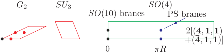
Figure 1: $G_{2}\oplus SU(3)\oplus SO(4)$ lattice with $\mathbb{Z}_{2}$ fixed points. The $T_{3}$ twisted sector states sit at these fixed points. The fixed point at the origin and the symmetric linear combination of the red (grey) fixed points in the $G_{2}$ torus have $\gamma=1$.

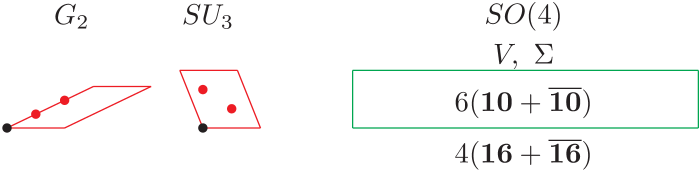
Figure 2: $G_{2}\oplus SU(3)\oplus SO(4)$ lattice with $\mathbb{Z}_{3}$ fixed points. The fixed point at the origin and the symmetric linear combination of the red (grey) fixed points in the $G_{2}$ torus have $\gamma=1$. The fields $V,\ \Sigma,\$ and $1\times({\bf 16}+{\bf\overline{16}})$ are bulk states from the untwisted sector. On the other hand, $6\times({\bf 10}+{\bf\overline{10}})$ and $3\times({\bf 16}+{\bf\overline{16}})$ are “bulk” states located on the $T_{2}/T_{4}$ twisted sector fixed points.

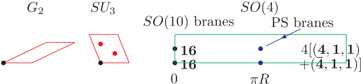
Figure 3: $G_{2}\oplus SU(3)\oplus SO(4)$ lattice with $\mathbb{Z}_{6}$ fixed points. The $T_{1}$ twisted sector states sit at these fixed points.

Massless states in 4d string models consist of those momentum vectors ${\bf P}$ and ${\bf r}$ ($\bf r$ are in the $SO(8)$ weight lattice) which satisfy the following mass-shell equations Dixon ; IMNQ ,

$$\frac{\alpha^{\prime}}{2}m_{R}^{2}=N^{k}_{R}+\frac{1}{2}\left|{\bf r}+k{\bf v}\right|^{2}+a^{k}_{R}=0\,,$$ (3)

$$\frac{\alpha^{\prime}}{2}m_{L}^{2}=N_{L}^{k}+\frac{1}{2}\left|{\bf P}+k{\bf X}\right|^{2}+a_{L}^{k}=0\,,$$ (4)

where $\alpha^{\prime}$ is the Regge slope, $N^{k}_{R}$ and $N^{k}_{L}$ are (fractional) numbers of the right- and left-moving (bosonic) oscillators, ${\bf X}={\bf V}+n_{3}{\bf W}_{3}+n_{2}{\bf W}_{2}+n_{2}^{\prime}{\bf W}_{2}^{\prime}$, and $a^{k}_{R}$, $a_{L}^{k}$ are the normal ordering constants,

$$a^{k}_{R} = -\frac{1}{2}+\frac{1}{2}\sum_{i=1}^{3}|{\widehat{kv_{i}}}|\left(1-|{\widehat{kv_{i}}}|\right)\,,$$

$$a_{L}^{k} = -1+\frac{1}{2}\sum_{i=1}^{3}|{\widehat{kv_{i}}}|\left(1-|{\widehat{kv_{i}}}|\right)\,,$$ (5)

with $\widehat{kv_{i}}={\rm mod}(kv_{i},1)$.

These states are subject to a generalized Gliozzi-Scherk-Olive (GSO) projection ${\cal P}=\frac{1}{6}\sum_{\ell=0}^{5}\Delta^{\ell}$ IMNQ . For the simple case of the $k$-th twisted sector ($k=0$ for the untwisted sectors) with no Wilson lines ($n_{3}=n_{2}=n^{\prime}_{2}=0$) we have

$$\Delta=\gamma\phi\exp\left\{i\pi\biggl{[}(2{\bf P}+k{\bf X})\cdot{\bf X}-(2{\bf r}+k{\bf v})\cdot{\bf v}\biggr{]}\right\},$$ (6)

where $\phi$ are phases from bosonic oscillators. However, in the $\mathbb{Z}_{6}$ model, the GSO projector must be modified for the untwisted-sector and $T_{2,4}$, $T_{3}$ twisted-sector states in the presence of Wilson lines KRZ . The Wilson lines split each twisted sector into sub-sectors and there must be additional projections with respect to these sub-sectors. This modification in the projector gives the following projection conditions,

$${\bf P}\cdot{\bf V}-{\bf r}_{i}\cdot{\bf v}=\mathbb{Z}\,\,\,\,(i=1,2,3),\quad{\bf P}\cdot{\bf W}_{3},\,\,{\bf P}\cdot{\bf W}_{2},\,\,{\bf P}\cdot{\bf W}_{2}^{\prime}=\mathbb{Z},$$ (7)

for the untwisted-sector states, and

$$T_{2,4}:\,{\bf P}\cdot{\bf W}_{2},\,\,{\bf P}\cdot{\bf W}_{2}^{\prime}={\mathbb{Z}}\,,\qquad T_{3}:\,{\bf P}\cdot{\bf W}_{3}={\mathbb{Z}}\,,$$ (8)

for the $T_{2,3,4}$ sector states (since twists of these sectors have fixed torii). There is no additional condition for the $T_{1}$ sector states.

4. An orbifold GUT – heterotic string dictionary. We first implement the $\mathbb{Z}_{3}$ sub-orbifold twist, which acts only on the $G_{2}$ and $SU(3)$ lattices. The resulting model is a 6d gauge theory with ${\cal N}=2$ hypermultiplet matter, from the untwisted and $T_{2,4}$ twisted sectors. This 6d theory is our starting point to reproduce the orbifold GUT models. The next step is to implement the $\mathbb{Z}_{2}$ sub-orbifold twist. The geometry of the extra dimensions closely resembles that of the 6d orbifold GUTs. The $SO(4)$ lattice has four $\mathbb{Z}_{2}$ fixed points at $0$, $\pi R$, $\pi R^{\prime}$ and $\pi(R+R^{\prime})$, where $R$ and $R^{\prime}$ are the two axes of the lattice (see Figs. 1 and 3). When one varies the modulus parameter of the $SO(4)$ lattice such that the length of one axis ($R$) is much larger than the other ($R^{\prime}$) and the string length scale ($\ell_{s}$), the lattice effectively becomes the $S^{1}/\mathbb{Z}_{2}$ orbi-circle in the 5d orbifold GUT, and the two fixed points at $0$ and $\pi R$ have degree-2 degeneracies. Furthermore, one may identify the states in the intermediate $\mathbb{Z}_{3}$ model, i.e. those of the untwisted and $T_{2,4}$ twisted sectors, as bulk states in the orbifold GUTs.

Space-time supersymmetry and GUT breaking in string models work exactly as in the orbifold GUT models. First consider supersymmetry breaking. In the field theory, there are two gravitini in 4d, coming from the 5d (or 6d) gravitino. Only one linear combination is consistent with the space reversal, $y\rightarrow-y$; this breaks the ${\cal N}=2$ supersymmetry to that of ${\cal N}=1$. In string theory, the space-time supersymmetry currents are represented by those half-integral $SO(8)$ momenta (see footnote 3). The $\mathbb{Z}_{3}$ and $\mathbb{Z}_{2}$ projections remove all but two of them, ${\bf r}=\pm\frac{1}{2}(1,1,1,1)$; this gives ${\cal N}=1$ supersymmetry in 4d.

Now consider GUT symmetry breaking. As usual, the $\mathbb{Z}_{2}$ orbifold twist and the translational symmetry of the $SO(4)$ lattice are realized in the gauge degrees of freedom by degree-2 gauge twists and Wilson lines respectively. To mimic the 5d orbifold GUT example, we impose only one degree-2 Wilson line, ${\bf W}_{2}$, along the long direction of the $SO(4)$ lattice, ${\bf R}$. The gauge embeddings generally break the 5d/6d (bulk) gauge group further down to its subgroups, and the symmetry breaking works exactly as in the orbifold GUT models. This can clearly be seen from the following string theoretical realizations of the orbifold parities

$$P=p\,e^{2\pi i\,[{\bf P}\cdot{\bf V}_{2}-{\bf r}\cdot{\bf v}_{2}]}\,,\quad P^{\prime}=p\,e^{2\pi i\,[{\bf P}\cdot({\bf V}_{2}+{\bf W}_{2})-{\bf r}\cdot{\bf v}_{2}]}\,,$$ (9)

where ${\bf V}_{2}=3{\bf V}_{6}$, and $p=\gamma\phi$ can be identified with intrinsic parities in the field theory language. Since $2({\bf P}\cdot{\bf V}_{2}-{\bf r}\cdot{\bf v}_{2}),\,2{\bf P}\cdot{\bf W}_{2}=\mathbb{Z}$, by properties of the $E_{8}\times E_{8}$ and $SO(8)$ lattices, thus $P^{2}=P^{\prime 2}=1$, and Eq. (9) provides a representation of the orbifold parities. From the string theory point of view, $P=P^{\prime}=+$ are nothing but the projection conditions, $\Delta=1$, for the untwisted and $T_{2,4}$ twisted-sector states (see Eqs. (6), (7) and (8)).

To reaffirm this identification, we compare the masses of KK excitations derived from string theory with that of orbifold GUTs. The coordinates of the $SO(4)$ lattice are untwisted under the $\mathbb{Z}_{3}$ action, so their mode expansions are the same as that of toroidal coordinates. Concentrating on the ${\bf R}$ direction, the bosonic coordinate is $X_{L,R}=x_{L,R}+p_{L,R}(\tau\pm\sigma)+{\rm oscillator\,terms}$, with $p_{L}$, $p_{R}$ given by

$$p_{L}=\frac{m}{2R}+\left(1-\frac{1}{4}|{\bf W}_{2}|^{2}\right)\frac{n_{2}R}{\ell_{s}^{2}}+\frac{{\bf P}\cdot{\bf W}_{2}}{2R}\,,\qquad p_{R}=p_{L}-\frac{2n_{2}R}{\ell_{s}^{2}}\,,$$ (10)

where $m$ ($n_{2}$) are KK levels (winding numbers). The ${\mathbb{Z}}_{2}$ action maps $m$ to $-m$, $n_{2}$ to $-n_{2}$ and ${\bf W}_{2}$ to $-{\bf W}_{2}$, so physical states must contain linear combinations, $|m,n_{2}\rangle\pm|-m,-n_{2}\rangle$; the eigenvalues $\pm 1$ correspond to the first ${\mathbb{Z}}_{2}$ parity, $P$, of orbifold GUT models. The second orbifold parity, $P^{\prime}$, induces a non-trivial degree-2 Wilson line; it shifts the KK level by $m\rightarrow m+{\bf P}\cdot{\bf W}_{2}$. Since $2{\bf W}_{2}$ is a vector of the (integral) $E_{8}\times E_{8}$ lattice, the shift must be an integer or half-integer. When $R\gg R^{\prime}\sim\ell_{s}$, the winding modes and the KK modes in the smaller dimension of $SO(4)$ decouple. Eq. (10) then gives four types of KK excitations, reproducing the field theoretical mass formula in Eq. (2).

5. A three-generation PS model. To illustrate the above points, we consider an explicit three-generation PS model in the $\mathbb{Z}_{6}$ orbifold, with the following gauge twist and Wilson lines,

$${\bf V}_{6} = \frac{1}{6}\left(22200000\right)\left(11000000\right)\,,$$ (11)

$${\bf W}_{3} = \frac{1}{3}\left(21-100000\right)\left(02110000\right)\,,$$ (12)

$${\bf W}_{2} = \frac{1}{2}\left(10000111\right)\left(00000000\right)\,.$$ (13)

The unbroken gauge groups in 4d are $SU(4)\times SU(2)_{L}\times SU(2)_{R}\times SO(10)^{\prime}\times SU(2)^{\prime}\times U(1)^{5}$ (one of the Abelian groups is anomalous), and the untwisted- and twisted-sector matter states furnish the following irreducible representations of the PS gauge group (modulo singlets),

$$U_{1}: ({\bf 4},{\bf 2},{\bf 1})\,,$$

$$T_{1}: 2({\bf 4},{\bf 2},{\bf 1})+2(\bar{\bf 4},{\bf 1},{\bf 2})+4({\bf 4},{\bf 1},{\bf 1})+4(\bar{\bf 4},{\bf 1},{\bf 1})+8({\bf 1,2,1})+6({\bf 1,1,2})$$

$$+2({\bf 1,2,1;1,2})+2({\bf 1,1,2;1,2})\,,$$

$$T_{2}: 2(\bar{\bf 4},{\bf 1},{\bf 2})+({\bf 6},{\bf 1},{\bf 1})+({\bf 1},{\bf 2},{\bf 2})\,,\quad T_{4}:\,\,({\bf 4},{\bf 1},{\bf 2})+2({\bf 6},{\bf 1},{\bf 1})+2({\bf 1},{\bf 2},{\bf 2})\,,$$

$$T_{3}: 2({\bf 4},{\bf 1},{\bf 1})+2(\bar{\bf 4},{\bf 1},{\bf 1})+6({\bf 1,1,2})\,,$$ (14)

where we have suppressed all the Abelian charges. This model contains three chiral PS families, two from the $T_{1}$ sector and one from the untwisted and $T_{2,4}$ twisted sectors. Note the $T_{2,4}$ sectors also contain a $({\bf 4,1,2})+({\bf\bar{4},1,2})$ pair which can be used to spontaneously break PS to the standard model (SM). The complete matter spectrum can be found in Ref. KRZ . It is natural to identify the two lightest families with the $T_{1}$ sector states $({\bf 4,2,1})+({\bf\bar{4},1,2})$ located on the $SO(10)$ brane (see Fig. 3). (In fact, we do not yet understand the dynamics which breaks the apparent symmetry between these two states.) The third family is then identified with the bulk states in $U_{1}$ and $T_{2}$. However, for this identification to be consistent with limits on proton decay we need $R^{-1}\equiv M_{c}\gtrsim 10^{16}$ GeV. We return to this point below when we discuss gauge coupling unification.

Gauge symmetry breaking and matter fields of this model can be understood in the language of orbifold GUTs. The intermediate $\mathbb{Z}_{3}$ model has a GUT group $SO(10)\times SU(2)$ in the observable sector (modulo Abelian factors), and contains the following untwisted and twisted-sector matter states in 6d hypermultiplets

$$U\,{\rm sectors}: ({\bf 16,1})+({\bf 1,2}),$$

$$T\,{\rm sectors}: 3({\bf 16,1})+6({\bf 10,1})+15({\bf 1,2}).$$ (15)

These matter states are bulk states in the language of orbifold GUTs (see Fig. 2). Note that, with the above 6d gauge sector and matter hypermultiplets, the irreducible 6d $SO(10)$ anomalies cancel 6danomalies .

The ${\mathbb{Z}}_{2}$ orbifold twist ${\bf v}_{2}$ (represented in the gauge degrees of freedom with the shift $\bf V_{2}$) along with the Wilson line $\bf W_{2}$ generate the two orbifold parities, $P$ and $P^{\prime}$, in field theory. As discussed earlier the orbifold parities can be computed for the states in Eq. (15) using Eq. (9), and they are listed in Table 1.

Table 1: Parities of the bulk states, i.e. the states in the gauge, untwisted and $T_{2}/T_{4}$ twisted sectors (separated by the horizontal lines respectively). The sub-indices $\pm$ are intrinsic parities. The multiplicities represent the number of fixed points in the $G_{2}$ torus. All the states have been decomposed into PS representations.

Multiplicities	States	$P$	$P^{\prime}$	States	$P$	$P^{\prime}$
1	$V({\bf 15,1,1})$	$+$	$+$	$\Sigma({\bf 15,1,1})$	$-$	$-$
1	$V({\bf 1,3,1})$	$+$	$+$	$\Sigma({\bf 1,3,1})$	$-$	$-$
1	$V({\bf 1,1,3})$	$+$	$+$	$\Sigma({\bf 1,1,3})$	$-$	$-$
1	$V({\bf 6,2,2})$	$+$	$-$	$\Sigma({\bf 6,2,2})$	$-$	$+$
1	$H({\bf 4,2,1})$	$+$	$+$	$H^{c}({\bf\bar{4},2,1})$	$-$	$-$
1	$H({\bf\bar{4},1,2})$	$+$	$-$	$H^{c}({\bf 4,1,2})$	$-$	$+$
2	$H({\bf 4,2,1})_{+}$	$+$	$-$	$H^{c}({\bf\bar{4},2,1})_{+}$	$-$	$+$
2	$H({\bf\bar{4},1,2})_{+}$	$+$	$+$	$H^{c}({\bf 4,1,2})_{+}$	$-$	$-$
2	$H({\bf 6,1,1})_{+}$	$-$	$+$	$H^{c}({\bf 6,1,1})_{+}$	$+$	$-$
2	$H({\bf 1,2,2})_{+}$	$-$	$-$	$H^{c}({\bf 1,2,2})_{+}$	$+$	$+$
2	$H({\bf 6,1,1})_{+}$	$-$	$-$	$H^{c}({\bf 6,1,1})_{+}$	$+$	$+$
2	$H({\bf 1,2,2})_{+}$	$-$	$+$	$H^{c}({\bf 1,2,2})_{+}$	$+$	$-$
1	$H({\bf 4,2,1})_{-}$	$-$	$+$	$H^{c}({\bf\bar{4},2,1})_{-}$	$+$	$-$
1	$H({\bf\bar{4},1,2})_{-}$	$-$	$-$	$H^{c}({\bf 4,1,2})_{-}$	$+$	$+$
1	$H({\bf 6,1,1})_{-}$	$+$	$+$	$H^{c}({\bf 6,1,1})_{-}$	$-$	$-$
1	$H({\bf 1,2,2})_{-}$	$+$	$-$	$H^{c}({\bf 1,2,2})_{-}$	$-$	$+$
1	$H({\bf 6,1,1})_{-}$	$+$	$-$	$H^{c}({\bf 6,1,1})_{-}$	$-$	$+$
1	$H({\bf 1,2,2})_{-}$	$+$	$+$	$H^{c}({\bf 1,2,2})_{-}$	$-$	$-$

The first embedding removes massless states with orbifold parities $P=-$. Just like in the field theory example, the $SO(10)\times SU(2)$ gauge group is unbroken. The remaining matter states are $U_{1}:\,({\bf 16,1})$, $U_{2}:\,({\bf 1,2})$, $T_{2}:\,2({\bf 16,1})_{+}+2({\bf 10,1})_{-}+2({\bf 1,2})_{+}+4({\bf 1,2})_{-}$, $T_{4}:\,({\bf\overline{16},1})_{-}+4({\bf 10,1})_{+}+8({\bf 1,2})_{+}+({\bf 1,2})_{-}$, where the sub-indices represent intrinsic parities. The second embedding, on the other hand, removes states with parities $P^{\prime}=-$. It breaks the observable-sector gauge group to the PS group (this is also identical to the orbifold GUT model). Finally, massless matter fields in the untwisted and $T_{2},\,T_{4}$ twisted sectors of our $\mathbb{Z}_{6}$ model (Eq. (14)) are the intersections of those of the two inequivalent embeddings of the ${\mathbb{Z}}_{2}$ orbifold twist, i.e. the surviving massless states in the 4d effective theory have orbifold parities $P=P^{\prime}=+$ which agrees with field theoretical results.

In the $\mathbb{Z}_{6}$ model there are also states from the $T_{1}$ and $T_{3}$ twisted sectors. They are localized on the two sets of inequivalent fixed points of the $SO(4)$ lattice at $0$ and $\pi R$, and can be properly identified with the brane states in the orbifold GUT models. From the $SO(4)$ lattice point of view, these states divide into two sub-sectors, according to their winding numbers, $n_{2}=0$ and $n_{2}=1$, along the direction where the ${\bf W}_{2}$ Wilson line is imposed. The set of states with $n_{2}=0$ ($n_{2}=1$) furnish complete representations of the $SO(10)\times SU(2)$ (PS) group. They are the $SO(10)$ (PS) brane states in the language of orbifold GUTs (see Figs. 1 and 3).

The $T_{1,3}$ twisted-sector states, i.e, the brane states, however, are more tightly constrained than their orbifold GUT counterparts. In orbifold GUT models the only consistency requirement is chiral anomaly cancelation, thus one can add arbitrary numbers of matter fields in vector-like representations on the branes. String models, on the other hand, have to satisfy more stringent modular invariance conditions Dixon ; vafa (which, of course, guarantee the model is anomaly free, up to a possible Abelian anomaly LSW ). These conditions usually constrain the additional allowed matter in vector-like representations. For example, we obtain states transforming in $({\bf 4,1,1})+({\bf\bar{4},1,1})$, $({\bf 1,1,2})$ and $({\bf 1,2,1})$ representations of PS on the PS brane. We also obtain states transforming under the hidden gauge group $SO(10)^{\prime}\times SU(2)^{\prime}$. In addition, the modular invariance conditions for the gauge twists and Wilson lines also imply that we cannot project away all the color triplet Higgs $({\bf 6,1,1})$ in our three-generation string model. This feature is different from that of $SO(10)$ orbifold GUT models. These color triplets do not necessarily pose the usual doublet-triplet problem as in conventional 4d GUT models, since in our case the triplets $({\bf 6,1,1})$ and doublets $({\bf 1,2,2})$ have different quantum numbers (namely, their Abelian charges). Rather than a nuisance, the color triplets may actually facilitate the breaking of the PS symmetry to that of the SM. A detailed analysis of the Yukawa couplings, both at renormalizable and non-renormalizable levels, and breaking of the PS symmetry will be given in Ref. KRZ .

6. Gauge coupling unification. Finally we determine various mass scales in our model by requiring gauge coupling unification. It is highly non-trivial to compute gauge threshold corrections in string theory kaplunovsky in the presence of discrete Wilson lines, and they are only known numerically in certain cases Nilles . However, in the orbifold GUT limit $R\gg R^{\prime}\sim\ell_{s}$, we only need to keep contributions from the massless and KK modes (in the ${\bf R}$ direction) below the string scale $M_{s}$, and the computation can be done by a much simpler field theoretical method. Following Ref. DDG , we find KRZ

$$\frac{2\pi}{\alpha_{i}(\mu)}=\frac{2\pi}{\alpha_{s}}+b^{\rm MSSM}_{i}\ln\frac{M_{b}}{\mu}+(b^{\rm PS}_{++}+b_{\rm branes})_{i}\ln\frac{M_{s}}{M_{b}}-\frac{1}{2}(b^{\rm PS}_{++}+b^{\rm PS}_{--})_{i}\ln\frac{M_{s}}{M_{c}}+b^{SO(10)}\left(\frac{M_{s}}{M_{c}}-1\right)\,,$$ (16)

for $i=1,2,3$, where $M_{b}$ and $M_{c}$ are the breaking scale of PS to the SM and the compactification scale respectively, $\alpha_{s}$ is the $SO(10)$ gauge coupling at the string scale, and $M_{s}\equiv 2/\sqrt{\alpha^{\prime}}=\sqrt{\alpha_{s}/2}\,M_{\rm pl}$ with $M_{\rm pl}\simeq 1.2\times 10^{19}$ GeV the Planck mass kaplunovsky . In this calculation, we have assumed $M_{b}\ll M_{c}$ so that the effect of symmetry breaking to the KK masses can be neglected. We have also assumed gauge threshold corrections from particle mass splittings at the breaking scale $M_{b}$ are negligible. The third term on the RHS includes the running due to massless modes as well as those “would be” massless states obtaining mass at $M_{b}$. The last term is the contribution of all bulk modes and characterizes the power-law running of gauge couplings in 5d. Finally, the fourth term on the RHS takes care of over-countings of the contributions from massless modes with $++$ and $--$ parities.

In Eq. (16), $b_{i}^{\rm MSSM}=(\frac{33}{5},1,-3)$ is the MSSM beta function coefficient (including one pair of Higgs doublets). Values of other beta function coefficients and the scales $M_{b}$ and $M_{c}$ depend on the field content below the string scale. As an example we assume 4 (2) bulk hypermultiplets in the ${\bf 16}+{\bf\overline{16}}$ (${\bf 10}+{\bf\overline{10}}$) representations (see Eq. (15)) and 4 pairs of $({\bf 4,1,1})+({\bf\bar{4},1,1})$ on the PS brane (see Eq. (14)) contribute to the running from $M_{c}$ or $M_{b}$ to $M_{s}$ (all other states are assumed to get mass at $M_{s}$). We then have $b_{++}^{\rm PS}+b_{\rm branes}=\frac{1}{2}(b_{++}^{\rm PS}+b_{--}^{\rm PS})=(\frac{22}{5},2,2)$ and $b^{SO(10)}=4$. From the point of view of an effective 4d GUT theory we have the following equations

$$\frac{2\pi}{\alpha_{i}(\mu)}\simeq\frac{2\pi}{\alpha_{G}}+b^{\rm MSSM}_{i}\ln\frac{M_{G}}{\mu}+6\,\delta_{i3}\,,$$ (17)

where the last factor represents the threshold corrections at the GUT scale $M_{G}\simeq 3\times 10^{16}$ GeV necessary to fit the low energy data. Matching Eqs. (16) and (17) at $M_{b}$, we find $M_{b}\simeq e^{-3/2}M_{G}\simeq 6.7\times 10^{15}$ GeV and $M_{c}\simeq e^{2}M_{G}\simeq 2.2\times 10^{17}$ GeV. The string scale and gauge coupling are $M_{s}\simeq 2.0\times 10^{18}$ GeV, $\alpha_{s}\simeq 0.06$. (The latter result is subject to scheme-dependent threshold corrections at $M_{s}$ and thus must await a true stringy calculation for confirmation.) We note that it is safe to identify the two $SO(10)$-brane states in the $\bf 16$ representation (see Fig. 3) as the lightest two generations of matter, since the compactification scale $M_{c}$ is large enough to sufficiently suppress dimension-6 operator contributions to proton decay. (We do not yet understand the contributions from dimension-5 operators due to color triplet exchanges; they depend on the precise nature of Yukawa couplings and are left for future investigations.) With the above mass scales, we find the string dilaton coupling $\sim M_{c}/\alpha_{s}M_{s}\sim{\cal O}(1)$, so the string interaction is in between the perturbative and non-perturbative regimes and might have very interesting physical implications.

Acknowledgments. T. K. was supported in part by the Grant-in-Aid for Scientific Research (#14540256) and the Grant-in-Aid for the 21st Century COE “The Center for Diversity and Universality in Physics” from Ministry of Education, Science, Sports and Culture of Japan. S. R. and R.-J. Z. were supported in part by DOE grants DOE-ER-01545-856 and DE-FG02-95ER40893 respectively. They also wish to express their gratitude to the Institute for Advanced Study, where initial stages of this work were performed, for partial financial support. Finally, S. R. acknowledges stimulating discussions with E. Witten and W. Buchmüller and R.-J. Z. thanks G. Kane for encouragement and advice.

References

- (1) Y. Kawamura, Prog. Theor. Phys. 103, 613 (2000); G. Altarelli and F. Feruglio, Phys. Lett. B 511, 257 (2001); L. Hall and Y. Nomura, Phys. Rev. D 64, 055003 (2001); Phys. Rev. D 66, 075004 (2002); A. Hebecker and J. March-Russell, Nucl. Phys. B 613, 3 (2001).
- (2) R. Dermíšek and A. Mafi, Phys. Rev. D 65, 055002 (2002); H. D. Kim and S. Raby, JHEP 0301, 056 (2003).
- (3) T. Asaka, W. Buchmüller and L. Covi, Phys. Lett. B 523, 199 (2001); L. J. Hall and Y. Nomura, hep-ph/0207079.
- (4) L. J. Dixon, J. A. Harvey, C. Vafa and E. Witten, Nucl. Phys. B 261, 678 (1985); Nucl. Phys. B 274, 285 (1986).
- (5) D. J. Gross, J. A. Harvey, E. J. Martinec and R. Rohm, Phys. Rev. Lett. 54, 502 (1985); Nucl. Phys. B 256, 253 (1985); Nucl. Phys. B 267, 75 (1986).
- (6) I. Antoniadis, G. K. Leontaris and J. Rizos, Phys. Lett. B 245, 161 (1990); G. K. Leontaris and N. D. Tracas, Phys. Lett. B 372, 219 (1996).
- (7) T. Kobayashi, S. Raby and R.-J. Zhang, to appear.
- (8) L. E. Ibáñez, J. E. Kim, H.-P. Nilles and F. Quevedo, Phys. Lett. B 191, 282 (1987); L. E. Ibáñez, J. Mas, H. P. Nilles and F. Quevedo, Nucl. Phys. B 301, 157 (1988); A. Font, L. E. Ibáñez, F. Quevedo and A. Sierra, Nucl. Phys. B 331, 421 (1990); D. Bailin, A. Love and S. Thomas, Phys. Lett. B 194, 385 (1987); Y. Katsuki, Y. Kawamura, T. Kobayashi, N. Ohtsubo, Y. Ono and K. Tanioka, Nucl. Phys. B 341, 611 (1990).
- (9) L. E. Ibáñez, H.-P. Nilles and F. Quevedo, Phys. Lett. B 187, 25 (1987).
- (10) C. Vafa, Nucl. Phys. B 273, 592 (1986).
- (11) T. Kobayashi and N. Ohtsubo, Phys. Lett. B 257, 56 (1991); Inter. J. Mod. Phys. A 9, 87 (1994).
- (12) L. Dixon, D. Friedan, E. Martinec and S. Shenker, Nucl. Phys. B 282, 13 (1987).
- (13) T. Asaka, W. Buchmüller and L. Covi, Nucl. Phys. B 648, 231 (2003).
- (14) A. N. Schellekens and N. P. Warner, Phys. Lett. B 181, 339 (1986); Nucl. Phys. B 287, 317 (1987); W. Lerche, A. N. Schellekens and N. P. Warner, Nucl. Phys. B 299, 91 (1988).
- (15) V. S. Kaplunovsky, Nucl. Phys. B 307, 145 (1988); L. Dixon, V. S. Kaplunovsky and J. Louis, Nucl. Phys. B 355, 649 (1991).
- (16) P. Mayr, H.-P. Nilles and S. Stieberger, Phys. Lett. B 317, 53 (1993).
- (17) K. R. Dienes, E. Dudas and T. Gherghetta, Phys. Lett. B 436, 55 (1998); Nucl. Phys. B 537, 47 (1999).