Abstract

The relativistic calculations of the electromagnetic form factors and static moments of $\rho$-meson are given in the framework of the relativistic Hamiltonian dynamics with different model wave functions. The impulse approximation is used. Lorentz covariance and conservation law for the electromagnetic current operator are taken into account.

Introduction

A new relativistic approach to electroweak properties of composite systems has been proposed in our recent papers [1, 2]. The approach is based on the use of the instant form (IF) of relativistic Hamiltonian dynamics (RHD). The detailed description of RHD can be found in the review [3]. Some other references as well as some basic equations of RHD approach are given in Ref.[1, 2].

In the paper [1] our approach was used to give a realistic calculation of electroweak properties of pion considered as composite quark–antiquark system. The electromagnetic form factor and the lepton decay constant were calculated for pion using different model wave functions for the relative motion of quarks in pion.

Now our aim is to describe the electromagnetic properties of more complicated systems, namely, $\rho$-meson as the composite system of two particles of spin 1/2 (quarks) with total spin one and total angular momentum one and with zero orbital momentum. The main problem is a construction of electromagnetic current operator satisfying standard conditions (Lorentz covariance, conservation law etc., see, e.g., Ref.[4]).

The basic point of our approach [1, 2] to the construction of the electromagnetic current operator is the general method of relativistic invariant parameterization of local operator matrix elements proposed as long ago as in 1963 by Cheshkov and Shirokov [5].

In fact, this parameterization is a realization of the Wigner–Eckart theorem for the Poincaré group and so it enables one for given matrix element of arbitrary tensor dimension to separate the reduced matrix elements (form factors) that are invariant under the Poincaré group. The matrix element of a given operator is represented as a sum of terms, each one of them being a covariant part multiplied by an invariant part. In such a representation a covariant part describes transformation (geometrical) properties of the matrix element, while all the dynamical information on the transition is contained in the invariant part – reduced matrix elements. In the case of composite systems these form factors appearing through the canonical parameterization are to be considered in the sense of distributions, that is they are generalized instead of classical functions. As was demonstrated in Ref.[1] this fact takes place even in nonrelativistic case. It is in terms of form factors that the electroweak properties of composite systems are described in the frame of the approach [1, 2].

In our approach some rather general problems arising in the description of composite quark models have been solved. For example, the description of electromagnetic properties of composite systems in terms of form factors in Ref.[1], in fact, solves the problem of construction of the electromagnetic current satisfying the conditions of translation invariance, Lorentz covariance, conservation law, cluster separability and equality of the composite system charge to the sum of constituents charges (charge nonrenormalizability).

Let us note that the importance of the problem of construction of electromagnetic current is actual not only for RHD but for all relativistic approaches to composite systems, including the field theoretical approaches [4, 6, 7, 8, 9, 10, 11].

Our calculations of the electromagnetic characteristics of $\rho$-meson are performed in the well known relativistic impulse approximation (IA). It means that the electromagnetic current of a composite system is a sum of one–particle currents of the constituents. It is worth emphasizing that in our method this approximation does not violate the standard conditions for the current. To–day a construction of relativistic impulse approximation without breaking of relativistic covariance and current conservation law is a common trend of different approaches [4, 8, 9, 11]. Let us note that in the present paper it is for the first time that such a construction has been realized for the case of nonzero spin in the frame of IF RHD. This is a variant of the relativistic impulse approximation formulated in terms of reduced matrix elements (see Ref. [1]) – the modified impulse approximation (MIA).

Using different model wave functions of quark relative motion we calculate the electromagnetic form factors and the static properties of $\rho$-meson supposing quarks to be in the $S$ state of relative motion. It is interesting to mention that relativistic effects occur to produce a nonzero quadrupole moment and quadrupole form factor. It is well known that in the nonrelativistic case the non–zero quadrupole form factor is caused by the presence of the $D$- wave and is zero otherwise.

The paper is organized as follows. In Sec.I the formalism developed in papers [1, 2] is used in the case of the system with total spin one and total angular momentum one. In terms of reduced matrix elements the so called modified impulse approximation (MIA)  [1] is formulated. In MIA $\rho$ – meson form factors are obtained explicitly.

In Sec.II the results of calculations of static properties and electromagnetic form factors of $\rho$ meson are discussed.

In Sec.III the conclusion is given.

1 Integral representation for the $\rho$-meson electromagnetic form factors

Let us consider the matrix element of the $\rho$-meson electromagnetic current. In our composite quark model the $u$- and $\bar{d}$– quarks are in the $S$ state of relative motion, that is $l=l^{\prime}=$ 0, with total spin one and total angular momentum one: $J=J^{\prime}=S=S^{\prime}=$1. This matrix element is given in the paper [2]:

$$\langle\vec{p}_{c}\,,m_{Jc}|j_{\mu}(0)|\vec{p}_{c}\,^{\prime}\,,m^{\prime}_{Jc}\rangle=\langle\,m_{Jc}|\,D^{1}(p_{c}\,,p^{\prime}_{c})\,\sum_{i=1,3}\,\tilde{\cal F}\,^{i}_{c}(t)\,\tilde{A}^{i}_{\mu}\,|m^{\prime}_{Jc}\rangle\;;$$ (1)

$$\tilde{\cal F}\,^{1}_{c}(t)=\tilde{f}^{c}_{10}+\tilde{f}^{c}_{12}\left\{[i{p_{c}}_{\nu}\,\Gamma^{\nu}(p^{\prime}_{c})]^{2}\right.\left.-\frac{1}{3}\,\hbox{Sp}[i{p_{c}}_{\nu}\,\Gamma^{\nu}(p^{\prime}_{c})]^{2}\right\}\frac{2}{\hbox{Sp}[{p_{c}}_{\nu}\,\Gamma^{\nu}(p^{\prime}_{c})]^{2}}\;,$$

$$\tilde{\cal F}\,^{3}_{c}(t)=\tilde{f}^{c}_{30}\;;$$ (2)

$$\tilde{A}^{1}_{\mu}=(p_{c}+p^{\prime}_{c})_{\mu}\;,\quad\tilde{A}^{3}_{\mu}=\frac{i}{M_{c}}\varepsilon_{\mu\nu\lambda\sigma}\,p_{c}^{\nu}\,p^{\prime}_{c}\,{}^{\lambda}\,\Gamma^{\sigma}(p^{\prime}_{c})\;,$$

here $p^{\prime}_{c}\,,p_{c}$ are 4-vectors of $\rho$-meson in initial and final states, $m^{\prime}_{Jc}\,,m_{Jc}$ are projections of the total angular momenta, $D^{1}(p_{c}\,,\,p^{\prime}_{c})$ is matrix of Wigner rotation, $\Gamma^{\nu}(p^{\prime}_{c})$ is 4-vector of spin, $M_{c}$ is $\rho$-meson mass, $\tilde{f}^{c}_{10}\,,\,\tilde{f}^{c}_{12}\,,$ $\tilde{f}^{c}_{30}$ are charge, quadrupole and magnetic form factors of $\rho$-meson respectively.

The representation (1), and (2) of the matrix element satisfies all the conditions for the composite system electromagnetic current [4].

The integral representations for the composite system form factors in Eq. (1), and (2) are obtained in the papers [1, 2]:

$$\tilde{f}^{c}_{in}(Q^{2})=\int\,d\sqrt{s}\,d\sqrt{s^{\prime}}\,\varphi(s)\,\tilde{G}_{in}(s,Q^{2},s^{\prime})\varphi(s^{\prime})\;,$$ (3)

here $\varphi(s)$ is wave function of quarks in RHD, $\tilde{G}_{in}(s,Q^{2},s^{\prime})$ is Lorentz covariant generalized function (reduced matrix element on the Poincaré group).

Our form factors in Eq. (2) can be written in terms of standard Sachs form factors for the system with the total angular momentum one. To do this let us write the parameterization of the electromagnetic current matrix element in the Breit frame (see, e.g., Ref. [12]):

$$\langle\vec{p}_{c}\,,m_{J}|j_{\mu}(0)|\vec{p}_{c}\,^{\prime}\,,m^{\prime}_{J}\rangle=G^{\mu}(Q^{2})\;,$$

$$G^{0}(Q^{2})=2p_{c0}\left\{(\vec{\xi}\,^{\prime}\vec{\xi}\,^{*})\,G_{C}(Q^{2})+\left[(\vec{\xi}\,^{*}\vec{Q})(\vec{\xi}\,^{\prime}\vec{Q})-\frac{1}{3}Q^{2}(\vec{\xi}\,^{\prime}\vec{\xi}\,^{*})\right]\,\frac{G_{Q}(Q^{2})}{2M_{c}^{2}}\right\}\;,$$

$$\vec{G}(Q^{2})=\frac{p_{c0}}{M_{c}}\left[\vec{\xi}^{\prime}\,(\vec{\xi}\,^{*}\vec{Q})-\vec{\xi}\,^{*}(\vec{\xi}\,^{\prime}\vec{Q})\right]\,G_{M}(Q^{2})\;.$$ (4)

Here $G_{C}\;,\;G_{Q}\;,\;G_{M}$ are the charge, quadrupole and magnetic form factors, respectively.

The polarization vector in the Breit frame has the following form:

$$\xi^{\mu}(\pm 1)=\frac{1}{\sqrt{2}}(0\;,\;\mp 1\;,\;-\,i\;,\;0)\;,\quad\xi^{\mu}(0)=(0\;,\;0\;,\;0\;,\;1)\;.$$ (5)

The variables in $\xi$ are total angular momentum projections.

In the Breit frame:

$$q^{\mu}=(p_{c}-p^{\prime}_{c})^{\mu}=(0\;,\;\vec{Q})\;,\quad p_{c}^{\mu}=(p_{c0}\;,\;\frac{1}{2}\vec{Q})\;,\quad p^{\prime}_{c}\,{}^{\mu}=(p_{c0}\;,\;-\frac{1}{2}\vec{Q})\;,$$ (6)

$$p_{c0}=\sqrt{M_{c}^{2}+\frac{1}{4}Q^{2}}\;,\quad\vec{Q}=(0\;,\;0\;,\;Q)\;.$$

Comparing Eq. (1) with Eq. (4) and taking into account the fact that in the Breit system $D^{1}_{m_{J}\,m^{\prime\prime}_{J}}(p_{c}\,,p_{c}^{\prime})=\delta_{m_{J}\,m^{\prime\prime}_{J}}\;,$ we have:

$$G_{C}(Q^{2})=\tilde{f}^{c}_{10}(Q^{2})\;,\quad G_{Q}(Q^{2})=\frac{2\,M_{c}^{2}}{Q^{2}}\,\tilde{f}^{c}_{12}(Q^{2})\;,$$

$$\quad G_{M}(Q^{2})=-\,M_{c}\,\tilde{f}^{c}_{30}(Q^{2})\;.$$ (7)

Let us use for (3) the modified impulse approximation formulated in terms of form factors $\tilde{G}_{iq}(s,Q^{2},s^{\prime})$. The physical meaning of this approximation is considered in detail in Ref. [1]. In the frame of MIA the invariant form factors $\tilde{G}_{iq}(s,Q^{2},s^{\prime})$ in (3) are changed by the free two–particle invariant form factors $g_{0i}(s,Q^{2},s^{\prime})\;(i=C,Q,M)$ describing the electromagnetic properties of the system of two free particles. So, the equations to be used for the calculation of the $\rho$–meson properties in MIA are the following:

$$G_{C}(Q^{2})=\int\,d\sqrt{s}\,d\sqrt{s^{\prime}}\,\varphi(s)\,g_{0C}(s\,,Q^{2}\,,s^{\prime})\,\varphi(s^{\prime})\;,$$

$$G_{Q}(Q^{2})=\frac{2\,M_{c}^{2}}{Q^{2}}\,\int\,d\sqrt{s}\,d\sqrt{s^{\prime}}\,\varphi(s)\,g_{0Q}(s\,,Q^{2}\,,s^{\prime})\,\varphi(s^{\prime})\;,$$ (8)

$$G_{M}(Q^{2})=-\,M_{c}\,\int\,d\sqrt{s}\,d\sqrt{s^{\prime}}\,\varphi(s)\,g_{0M}(s\,,Q^{2}\,,s^{\prime})\,\varphi(s^{\prime})\;.$$

The free two–particle invariant form factors can be calculated by the methods of relativistic kinematics and have the following form.

The charge free two–particle form factor:

$$g_{0C}(s,Q^{2},s^{\prime})=\frac{1}{3}\,R(s,Q^{2},s^{\prime})\,Q^{2}\,\times$$

$$\times\left\{(s+s^{\prime}+Q^{2})(G^{u}_{E}+G^{\bar{d}}_{E})\,\left[2\,\cos(\omega_{1}-\omega_{2})+\cos(\omega_{1}+\omega_{2})\right]-\right.$$

$$-\left.\frac{1}{M}\xi(s,Q^{2},s^{\prime})(G^{u}_{M}+G^{\bar{d}}_{M})\,\left[2\,\sin(\omega_{1}-\omega_{2})-\sin(\omega_{1}+\omega_{2})\right]\right\}\;.$$ (9)

The quadrupole free two–particle form factor:

$$g_{0Q}(s,Q^{2},s^{\prime})=\frac{1}{2}\,R(s,Q^{2},s^{\prime})\,Q^{2}\,\times$$

$$\times\left\{(s+s^{\prime}+Q^{2})(G^{u}_{E}+G^{\bar{d}}_{E})\,\left[\cos(\omega_{1}-\omega_{2})-\cos(\omega_{1}+\omega_{2})\right]-\right.$$

$$-\left.\frac{1}{M}\xi(s,Q^{2},s^{\prime})(G^{u}_{M}+G^{\bar{d}}_{M})\,\left[\sin(\omega_{1}-\omega_{2})+\sin(\omega_{1}+\omega_{2})\right]\right\}\;.$$ (10)

The magnetic free two–particle form factor:

$$g_{0M}(s,Q^{2},s^{\prime})=-\,{2}\,R(s,Q^{2},s^{\prime})\,\times$$

$$\times\left\{\xi(s,Q^{2},s^{\prime})(G^{u}_{E}+G^{\bar{d}}_{E})\,\sin(\omega_{1}-\omega_{2})+\right.$$

$$+\frac{1}{4M}(G^{u}_{M}+G^{\bar{d}}_{M})\left[(s+s^{\prime}+Q^{2})\,Q^{2}\left(\frac{3}{2}\cos(\omega_{1}-\omega_{2})+\frac{1}{2}\cos(\omega_{1}+\omega_{2})\right)\right.-$$

$$-\frac{1}{4}\xi(s,Q^{2},s^{\prime})\left[\beta(s,Q^{2},s^{\prime})+\beta(s^{\prime},Q^{2},s)\right]\times$$

$$\times\left[\sin(\omega_{1}-\omega_{2})-\sin(\omega_{1}+\omega_{2})\right]$$

$$-\frac{1}{2}\xi^{2}(s,Q^{2},s^{\prime})\left[\frac{1}{\sqrt{s^{\prime}}(\sqrt{s^{\prime}}+2\,M)}\right.+$$

$$\left.\left.\left.+\frac{1}{\sqrt{s}(\sqrt{s}+2\,M)}\right]\left[\cos(\omega_{1}-\omega_{2})+\cos(\omega_{1}+\omega_{2})\right]\right]\right\}\;.$$ (11)

In Eqs. (9)–(11):

$$R(s,Q^{2},s^{\prime})=\frac{(s+s^{\prime}+Q^{2})}{2\sqrt{(s-4M^{2})(s^{\prime}-4M^{2})}}\,\frac{\vartheta(s,Q^{2},s^{\prime})}{{[\lambda(s,-Q^{2},s^{\prime})]}^{3/2}}\frac{1}{\sqrt{1+Q^{2}/4M^{2}}}\;,$$

$$\xi(s,Q^{2},s^{\prime})=\sqrt{ss^{\prime}Q^{2}-M^{2}\lambda(s,-Q^{2},s^{\prime})}\;,$$

$$\beta(s,Q^{2},s^{\prime})=\frac{(\sqrt{s^{\prime}}+2\,M)(s-s^{\prime}+Q^{2})+(s^{\prime}-s+Q^{2})\sqrt{s^{\prime}}}{\sqrt{s^{\prime}}(\sqrt{s^{\prime}}+2\,M)}\;,$$

$\omega_{1}$ and $\omega_{2}$ are the Wigner rotation parameters:

$$\omega_{1}=\hbox{arctg}\frac{\xi(s,Q^{2},s^{\prime})}{M\left[(\sqrt{s}+\sqrt{s^{\prime}})^{2}+Q^{2}\right]+\sqrt{ss^{\prime}}(\sqrt{s}+\sqrt{s^{\prime}})}\;,$$

$$\omega_{2}=\hbox{arctg}\frac{\alpha(s,s^{\prime})\xi(s,Q^{2},s^{\prime})}{M(s+s^{\prime}+Q^{2})\alpha(s,s^{\prime})+\sqrt{ss^{\prime}}(4M^{2}+Q^{2})}\;,$$ (12)

$\alpha(s,s^{\prime})=2M+\sqrt{s}+\sqrt{s^{\prime}}$, $\vartheta(s,Q^{2},s^{\prime})=\theta(s^{\prime}-s_{1})-\theta(s^{\prime}-s_{2})$, $\theta$ is the step–function:

$$\theta(x)=\left\{\begin{array}[]{lll}0\;,&x\;\leq\;0\\ 1\;,&x\;>\;0\;,\\ \end{array}\right.$$

$$s_{1,2}=2M^{2}+\frac{1}{2M^{2}}(2M^{2}+Q^{2})(s-2M^{2})\mp\frac{1}{2M^{2}}\sqrt{Q^{2}(Q^{2}+4M^{2})s(s-4M^{2})}\;,$$

$M$ is the mass of the $u$- and $\bar{d}-$quarks. The functions $s_{1,2}(s,Q^{2})$ give the kinematically available region in the plane $(s,s^{\prime})$. $G^{u,\bar{d}}_{E,M}=G^{u,\bar{d}}_{E,M}(Q^{2})$ are Sachs form factors of $u$- and $\bar{d}-$quarks.

The non-relativistic limit of equations (8) gives the following forms of the form factors:

$$G_{C}(Q^{2})=\left(G^{u}_{E}(Q^{2})+G^{\bar{d}}_{E}(Q^{2})\right)\,I(Q^{2})\;,\quad G_{Q}(Q^{2})=0\;,$$

$$G_{M}(Q^{2})=\frac{M_{\rho}}{M}\left(G^{u}_{M}(Q^{2})+G^{\bar{d}}_{M}(Q^{2})\right)\,I(Q^{2})\;,$$ (13)

$$I(Q^{2})=\int\,k^{2}\,dk\,k^{\prime}\,{}^{2}\,dk^{\prime}\,u(k)\,g_{NR}(k,Q^{2},k^{\prime})u(k^{\prime})\;,$$

$$g_{NR}(k,Q^{2},k^{\prime})=\frac{1}{k\,k^{\prime}\,Q}\,\left[\theta\left(k^{\prime}-\left|k-\frac{Q}{2}\right|\right)-\theta\left(k^{\prime}-k-\frac{Q}{2}\right)\right]\;.$$

Let us note that the obtained result (13) coincides with the one derived in standard non-relativistic calculations for composite system form factors in the impulse approximation [13]. So, Eq. (8) can be considered as a relativistic generalization of the equations of Ref. [13].

2 $\rho$-meson electromagnetic structure

Electroweak properties of composite hadron systems were described in the RHD approach in a number of papers. The most popular approach in the frame of RHD is the light–front dynamics [7, 14, 15, 16, 17, 18, 19]. Recently some calculations in the frame of instant form [20, 21] and point form dynamics [22] have appeared. The $\rho$ – meson electromagnetic structure was calculated in Refs. [14, 15, 23, 24, 25] in the light–front dynamics approach.

In this section we make use of the results of the previous sections to calculate the $\rho$ – meson electromagnetic properties.

The $\rho$ – meson electromagnetic form factors are calculated using Eqs. (8), (9)–(12) in MIA. The wave functions in sense of RHD in Eq. (8) at $J=S=1\;,l=0$ are defined by the following expression (see e.g. [1]):

$$\varphi(k(s))=\sqrt[4]{s}\,u(k)\,k\;,\quad k=\frac{1}{2}\sqrt{s-4\,M^{2}}\;$$ (14)

and is normalized by the condition:

$$\int\,u^{2}(k)\,k^{2}\,dk=1\;,$$ (15)

here $u(k)$ is a model wave function.

For the description of the relative motion of quarks (as in Ref. [1] in the case of pion) in Eq. (14) the following phenomenological wave functions are used:

1. A Gaussian or harmonic oscillator (HO) wave function (see, e.g., Ref. [19])

$$u(k)=N_{HO}\,\hbox{exp}\left(-{k^{2}}/{2\,b^{2}}\right).$$ (16)

2. A power-law (PL) wave function [18]:

$$u(k)=N_{PL}\,{(k^{2}/b^{2}+1)^{-n}}\;,\quad n=2\;,3\;.$$ (17)

3. The wave function with linear confinement from Ref. [26]:

$$u(r)=N_{T}\,\exp(-\alpha r^{3/2}-\beta r)\;,\quad\alpha=\frac{2}{3}\sqrt{2\,M_{r}\,a}\;,\quad\beta=M_{r}\,b\;,$$ (18)

here $a\;,b$ are the parameters of linear and Coulomb parts of potential respectively, $M_{r}$ is the reduced mass of the two–particle system.

For Sachs form factors of quarks in Eqs. (10) we have:

$$G^{q}_{E}(Q^{2})=e_{q}\,f_{q}(Q^{2})\;,\quad G^{q}_{M}(Q^{2})=(e_{q}+\kappa_{q})\,f_{q}(Q^{2})\;,$$ (19)

where $e_{q}$ is the quark charge and $\kappa_{q}$ is the quark anomalous magnetic moment. For $f_{q}(Q^{2})$ the form of Ref. [27] is used:

$$f_{q}(Q^{2})=\frac{1}{1+\ln(1+\langle r^{2}_{q}\rangle Q^{2}/6)}\;.$$ (20)

Here $\langle r^{2}_{q}\rangle$ is the mean square radius (MSR) of constituent quark.

The details describing the cause of the choice (20) for the function $f_{q}(Q^{2})$ can be found in Ref. [27] (see also Ref. [1]) and are based on the fact that this form gives the asymptotics of the pion form factor as $Q^{2}\to\infty$ that coincides with the QCD asymptotics [28].

So, for the calculations we use a standard set of parameters of constituent quark model. The structure of the constituent quark is described by the following parameters: $M_{u}=M_{\bar{d}}=M$ is the constituent quark mass, $\kappa_{u}\;,\;\kappa_{\bar{d}}$ are the constituent quarks anomalous magnetic moments, $\langle\,r^{2}_{u}\rangle=\langle\,r^{2}_{\bar{d}}\rangle=\langle\,r^{2}_{q}\rangle$ is the quark MSR. The interaction of quarks in $\rho$ meson is characterized by wave functions (16) – (18) with the parameters $b\;,\;\alpha\;,\;\beta$.

The parameters were fixed in our calculation as follows. We use $M$=0.25 GeV [29] for the quark mass. The quark anomalous magnetic moments enter the equations through the sum ($\kappa_{u}+\kappa_{\bar{d}}$) and we take $\kappa_{u}+\kappa_{\bar{d}}$ = 0.09 in natural units following [30].

For the quark MSR we use the relation $\langle r^{2}_{q}\rangle\simeq 0.3/M^{2}$ [31, 32].

The parameter $b$ in the Coulomb part of the potential in Eq. (18) is $b$ = 0.7867. This gives the value $\alpha_{S}$ = 0.59 for systems of light quarks. We choose the parameters $b$ in Eqs. (16) and (17) and $a$ in Eq. (18) so as to fit the MSR of $\rho$ meson.

The $\rho$ – meson MSR is given by the equation $\langle r^{2}_{\rho}\rangle-\langle r^{2}_{\pi}\rangle$ = 0.11$\pm$0.06 fm² [31, 32]. For the pion MSR the experimental data [33] is taken: $\langle r^{2}_{\pi}\rangle^{1/2}$ = 0.657$\pm$0.012 fm.

We use the following relation for the $\rho$-meson MSR:

$$\langle\,r^{2}_{\rho}\rangle=-6\,G^{\prime}_{C}(0)\;.$$ (21)

The $\rho$ – meson mass in Eq. (8) is taken from Ref. [34]: $M_{c}=M_{\rho}$ = 763.0$\pm$1.3 MeV.

The magnetic $\mu_{\rho}$ and the quadrupole $Q_{\rho}$ moments of $\rho$ meson were calculated using the relations [12]:

$$G_{M}(0)=\frac{M_{\rho}}{M}\,\mu_{\rho}\;,\quad G_{Q}(0)=M_{\rho}^{2}\,Q_{\rho}\;.$$ (22)

The static limit in Eqs. (8) gives the following relativistic expressions for moments:

$$\mu_{\rho}=\frac{1}{2}\,\int_{2M}^{\infty}\,d\sqrt{s}\,\frac{\varphi^{2}(s)}{\sqrt{s-4\,M^{2}}}\,\left\{1-L(s)+(\kappa_{u}+\kappa_{\bar{d}})\left[1-\frac{1}{2}\,L(s)\right]\right\}\;,$$ (23)

$$Q_{\rho}=-\,\int_{2M}^{\infty}\,d\sqrt{s}\,\frac{\varphi^{2}(s)}{\sqrt{s}}\,\left[\frac{M}{\sqrt{s}+2\,M}+\kappa_{u}+\kappa_{\bar{d}}\right]\,\frac{L(s)}{4M\sqrt{s-4M^{2}}}\;,$$ (24)

$$L(s)=\frac{2\,M^{2}}{\sqrt{s-4\,M^{2}}\,(\sqrt{s}+2\,M)}\,\left[\frac{1}{2\,M^{2}}\sqrt{s\,(s-4\,M^{2})}+\right.$$

$$+\left.\ln\,\frac{\sqrt{s}-\sqrt{s-4\,M^{2}}}{\sqrt{s}+\sqrt{s-4\,M^{2}}}\right]\;.$$

Let us note that the nonzero $\rho$ – meson quadrupole moment appears due to the relativistic effect of Wigner spin rotation of quarks only. So, measuring of the quadrupole moment can be a test of the relativistic invariance in the confinement region.

The Wigner rotation contributes to the magnetic moment, too. Without spin rotation ($\omega_{1}=\omega_{2}$ = 0 in (12)) we have for the magnetic moment:

$$\tilde{\mu}_{\rho}=\frac{1}{2}(1+\kappa_{u}+\kappa_{\bar{d}})\,\int_{2M}^{\infty}\,d\sqrt{s}\,\frac{\varphi^{2}(s)}{\sqrt{s-4\,M^{2}}}\,\left\{1-\frac{1}{2}\,L(s)\right\}\;.$$ (25)

To estimate the contribution of Wigner rotation we have calculated the $\rho$-meson MSR $\langle\,\tilde{r}_{\rho}^{2}\rangle$ without spin rotation ($\omega_{1}=\omega_{2}$ = 0 in Eqs. (8), (9), (12), (21)).

To estimate the contribution of the relativistic effects to the $\rho$ – meson electromagnetic structure the non-relativistic calculation of electromagnetic form factors, MSR $\langle\,r^{2}_{NR}\rangle$ and magnetic moment $\mu_{\rho\,NR}$ was performed using Eqs. (13), (21), (22).

The calculation of the non-relativistic magnetic moments using Eq. (22) gives the following result which does not depend on the model wave functions:

$$\mu_{\rho\,NR}=1+\kappa_{u}+\kappa_{\bar{d}}\;.$$ (26)

The values of parameters being fixed before we obtain $\mu_{\rho\,NR}$ = 1.09.

The results of the calculation of the $\rho$ – meson statical moments are given in the Table I. The relativistic results for the same parameters but without Wigner spin rotation ($\omega_{1}=\omega_{2}$ = 0 in Eq. (12)), as well as of non-relativistic calculation are given, too. The number of significant digits is chosen so as to demonstrate the extent of the model dependence of the calculations.

Table 1: The $\rho$ – meson statical moments obtained with the different model wave functions (16) – (18). $\langle\,r^{2}_{NR}\rangle$ is nonrelativistic MSR, $\langle\,\tilde{r}_{\rho}^{2}\rangle$ is relativistic MSR without spin rotation contribution, $\mu_{\rho}$ is relativistic magnetic moment (23), $\tilde{\mu}_{\rho}$ is relativistic magnetic moment without spin rotation (25), $Q_{\rho}$ is quadrupole moment (24). The wave functions parameters are obtained from the fitting of $\rho$ – meson MSR obtained through the relativistic calculation with spin rotation, $\langle r^{2}_{\rho}\rangle-\langle r^{2}_{\pi}\rangle$ = 0.11$\pm$0.06 fm² [31, 32]. The pion MSR was taken from the experimental data [33]: $\langle r^{2}_{\pi}\rangle^{1/2}$ = 0.657$\pm$0.012 fm. The magnetic moments are in natural units, the quadrupole moments and MSR are in fm². The parameters $b$ in (16) and (17) – are in GeV and $a$ in (18) – in GeV². The values of other parameters are given in the text. The number of the significant digits is chosen so as to demonstrate the extent of model dependence of calculations.

Wave
functions	$b\;,a$	$\langle\,r^{2}_{NR}\rangle$	$\langle\,\tilde{r}_{\rho}^{2}\rangle$	$\mu_{\rho}$	$\tilde{\mu}_{\rho}$	$Q_{\rho}$
(16)	0.231	0.275	0.731	0.852	0.966	-0.0065
(17) n=2	0.302	0.319	0.711	0.864	0.972	-0.0059
(17) n=3	0.430	0.305	0.710	0.866	0.973	-0.0061
(18)	0.028	0.301	0.711	0.865	0.973	-0.0061

As one can see from the table the contributions of the spin rotation to the magnetic moment and to MSR depend weakly on the model for the quarks interaction in $\rho$ meson. This contribution to the MSR is 24%–26% and is negative. This result differs from that of the paper [14] where the contribution of spin rotation (Melosh rotation) to MSR calculated in the frame of light–front dynamics is positive.

The spin rotation contribution to the magnetic moment in our calculations is 11%–12% and is negative, too. The total relativistic corrections to MSR in our approach are positive and enlarge the non-relativistic value essentially – almost twice in the case of the model (16) and for 70% – 80% for the models (17), (18).

The total relativistic corrections for the magnetic moment as compared to the non-relativistic result (see Eq. (26)) are negative and have the value of 21%–22%. Let us note, that in the light–front dynamics approach [15] a different result was obtained: the positive relativistic correction of the value of 10% to the magnetic moment.

The results of calculations for the $\rho$ – meson electromagnetic form factors are represented in Fig.1–4.

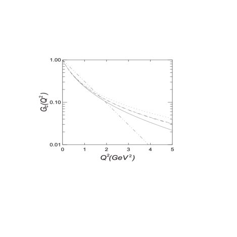
Figure 1: The results of the calculations of the $\rho$-meson charge form factor with different model wave functions. The values of the parameters are given in the Table I. The solid line represents the relativistic calculation with the wave function (16), the dashed line – with (17) for $n=$ 3, dash–dot–line – with (18), dotted line – with (17) for $n=$ 2, dot–dot–dash-line – the non-relativistic calculation with (16).

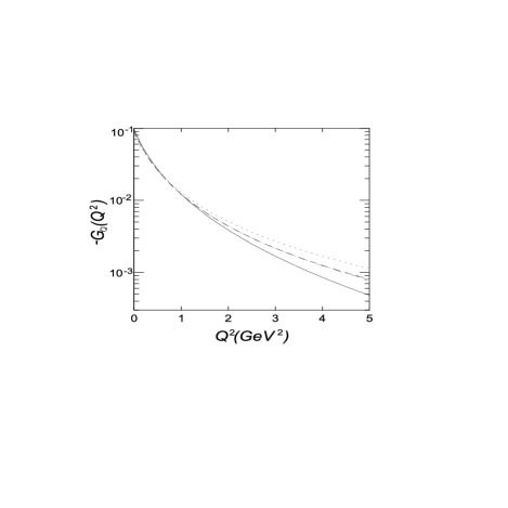
Figure 2: The results of the calculations of the $\rho$-meson quadrupole form factor with different model wave functions, legend as in Fig.1

Figure 3: The results of the calculations of the $\rho$-meson magnetic form factor with different model wave functions, legend as in Fig.1

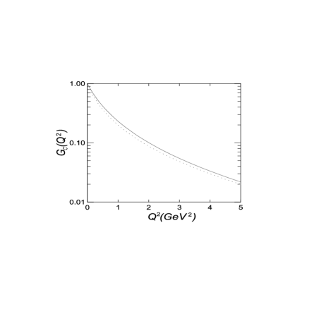
Figure 4: The contribution of the relativistic spin rotation effect. The results of the relativistic calculation of the $\rho$-meson charge form factor with the wave function (16) using the same parameters as in Fig.1. Solid line represents the relativistic calculation with spin rotation, dotted line – the relativistic calculation without spin rotation.

Let us note that our charge form factor has no dip in contrast with the results of the paper [15]. The relativistic corrections in our approach diminish essentially the rate of the decreasing of the charge and magnetic form factors at large values of momentum transfer. We demonstrate in the figures the case of the model (16) with the exponential decreasing of the nonrelativistic form factors with the increasing $Q^{2}$. The nonrelativistic quadrupole form factor is zero in the absence of the $D$–state in the two–particle system.

In Fig.4 the contribution of Wigner rotation of quark spins to the $\rho$ – meson charge form factor is shown. This contribution depends weakly on the momentum transfer in the range from 1 to 5 GeV² and its value is approximately 10%.

3 Conclusion

The electromagnetic form factors, quadrupole and magnetic moments, and MSR of the $\rho$-meson were calculated in the framework of the instant form of relativistic Hamiltonian dynamics (RHD).

The special method of construction of the electromagnetic current matrix elements for the relativistic two–particle composite systems with nonzero total angular momentum is used to obtain the integral representation for the electromagnetic form factors.

The modified impulse approximation (MIA) — with the physical content of the relativistic impulse approximation — is formulated in terms of reduced matrix elements on Poincaré group. MIA conserves Lorentz covariance of electromagnetic current and the current conservation law.

A reasonable description of the static moments and the electromagnetic form factors of $\rho$ meson is obtained in the developed formalism. A number of relativistic effects are obtained, for example, the nonzero quadrupole moment (in the case of $S$ state) due to the relativistic Wigner spin rotation.

So, it is shown that the instant form of RHD can be used to obtain an adequate description of the electroweak properties of composite systems with nonzero total angular momentum.

This work was supported in part by the Program ”Russian Universities–Basic Researches” (Grant No. 02.01.013) and Ministry of Education of Russia (Grant No. E02-3.1-34).

References

- [1] A.F. Krutov and V.E. Troitsky, Phys.Rev.C 65, 045501 (2002).
- [2] A.F. Krutov and V.E. Troitsky, Phys.Rev.C 68, 018501 (2003).
- [3] B.D. Keister and W. Polyzou, Adv. Nucl. Phys. 20, 225 (1991).
- [4] F.M. Lev, Ann. Phys. (N.Y.) 237, 355 (1995).
- [5] A.A. Cheshkov and Yu.M. Shirokov, Zh. Eksp. Teor. Fiz. 44, 1982 (1963).
- [6] F. Gross and D.O. Riska, Phys. Rev. C 36, 1928 (1987); H. Ito, W.W. Buck, and F. Gross, ibid. 43, 2483 (1991); F. Gross and H. Henning, Nucl. Phys. A537, 344 (1992); F. Coester and D.O. Riska, Ann. Phys. (N.Y.) 234, 141 (1994).
- [7] P.L. Chung, F. Coester, B.D. Keister, and W.N. Polyzou, Phys. Rev. C 37, 2000 (1988).
- [8] J.W. Van Orden, N. Devine, and F. Gross, Phys. Rev. Lett. 75, 4369 (1995).
- [9] F.M. Lev, E. Pace, and G. Salmé, Nucl. Phys. A641, 229 (1998).
- [10] J.P.B.C. de Melo, J.H.O. Sales, T. Frederico, and P.U. Sauer, Nucl. Phys. A631, 574 (1998).
- [11] W.H. Klink, Phys. Rev. C 58, 3587 (1998).
- [12] R.G. Arnold, C.E. Carlson, and F. Gross, Phys. Rev. C 21, 1426 (1980).
- [13] G.E. Brown and A.D. Jackson, The Nucleon–Nucleon Interaction (North–Holland, Amsterdam, 1976).
- [14] B.D. Keister, Phys. Rev.D 49, 1500 (1994).
- [15] F. Cardarelli, I.L. Grach, I.M. Narodetskii, G. Salmé , and S. Simula, Phys. Lett. B 349, 393 (1995).
- [16] I.L. Grach and L.A. Kondratyuk, Yad. Fiz. 39, 316 (1984) [Sov. J. Nucl. Phys. 39, 198 (1984)].
- [17] M.V. Terentyev, Yad. Fiz. 24, 207 (1976); I.G. Aznauryan and N.L. Ter-Isaakyan, Yad. Fiz 31, 1680 (1980); W. Jaus, Phys. Rev. D 44, 2851 (1991); J. Carbonell and V.A. Karmanov, Eur.Phys.J. A 6, 9 (1999); F.M. Lev, E. Pace, and G. Salmé, Phys. Rev. C 62, 064004 (2000).
- [18] F. Schlumpf, Phys.Rev. D 50, 6895 (1994).
- [19] P.L. Chung, F. Coester, and W.N. Polyzou, Phys. Lett. B 205, 545 (1988).
- [20] A.F. Krutov and V.E. Troitsky, J. Phys. G 19, L127 (1993); E.V. Balandina, A.F. Krutov, and V.E. Troitsky, J. Phys. G 22, 1585 (1996); A.F. Krutov, Yad. Fiz. 60, 1442 (1997) [Phys. At. Nucl. 60, 1305 (1997)]; E.V. Balandina, A.F. Krutov, V.E. Troitsky, and O.I. Shro, Yad. Fiz. 63, 301 (2000) [Phys. At. Nucl. 63, 244 (2000)].
- [21] J. Charles, A. Le Yaouanc, L. Oliver, O. Pène, and J.-C. Raynal, Phys. Lett. B 451, 187 (1999).
- [22] T.W. Allen and W.H. Klink, Phys. Rev. C 58, 3670 (1998); V.V. Andreev, Vestsi Nats. Akad. Navuk Belarusi, Ser. Fiz.-Mat. Navuk 2, 93 (2000); T.W. Allen, W.H. Klink, and W.N. Polyzou, Phys. Rev. C 63, 034002 (2001).
- [23] V.A. Karmanov, Nucl. Phys. A 608, 316 (1996).
- [24] D. Melikhov and S. Simula, Phys. Rev. C 65, 094043 (2002).
- [25] S. Simula, Phys. Rev. C 66, 035201 (2002).
- [26] H. Tezuka, J. Phys. A 24, 5267 (1991).
- [27] A.F. Krutov and V.E. Troitsky, Teor. Mat. Fiz. 116, 215 (1998) [Theor. Math. Phys. 116, 907 (1998)].
- [28] V.A. Matveev, R.M. Muradyan, and A.N. Tavkhelidze, Lett. Nuovo Cim. 7, 719 (1973), 15, 907 (1973); S. Brodsky and G. Farrar, Phys. Rev. Lett. 31, 1153 (1973).
- [29] A.F. Krutov and V.E. Troitsky, Eur. Phys. J. C 20, 71 (2001).
- [30] S.B. Gerasimov, JINR Report No. E2–89–837, Dubna, 1989; Phys.Lett. B 357, 666 (1995).
- [31] F. Cardarelli, I.L. Grach, I.M. Narodetskii, E. Pace, G. Salmé, and S. Simula, Phys. Rev. D 53, 6682 (1996).
- [32] U. Vogl, M. Lutz, S. Klimt, and W. Weise, Nucl. Phys. A516, 469 (1990); B. Povh and J. Hüfner, Phys. Lett. B 245, 653 (1990); S.M. Troshin and N.E. Tyurin, Phys. Rev. D 49, 4427 (1994).
- [33] S.R. Amendolia et al., Phys. Lett. B 146, 116 (1984).
- [34] A. Abele et al., Phys. Lett. B 469, 270 (1999).