Les Houches Guidebook to Monte Carlo Generators
for Hadron Collider Physics

Abstract

Recently the collider physics community has seen significant advances in the formalisms and implementations of event generators. This review is a primer of the methods commonly used for the simulation of high energy physics events at particle colliders. We provide brief descriptions, references, and links to the specific computer codes which implement the methods. The aim is to provide an overview of the available tools, allowing the reader to ascertain which tool is best for a particular application, but also making clear the limitations of each tool.

Compiled by the Working Group on Quantum ChromoDynamics and the Standard Model for the Workshop “Physics at TeV Colliders”, Les Houches, France, May 2003.

1 INTRODUCTION 

The complexity and number of simulation programs for hadron colliders has grown considerably with the prospects of LHC physics approaching and Tevatron Run II results coming in. With these programs has come a shift towards increased modularity. A physicist analysing hadron collider data often obtains the most accurate theoretical predictions by combining components of many different simulation programs—minimum bias from one generator, the signal process from another, and yet more programs for background generation. This sort of diversification is also happening for the generation of a single process. It is becoming feasible to use one program to produce a hard process, another to evolve the event through a parton shower algorithm, and perhaps a third to hadronize the coloured products of the shower. With this sort of modularity, the complexity of Monte Carlo simulation tools is reaching that of a complicated detector system. At the same time the expertise needed by the users is increasing. At the very start of a physics analysis, the experimenter is confronted with a simple question, which Monte Carlo tools are best suited to map the theoretical prediction for my measurement onto the experimental result?

The goal for this guidebook is to provide users inexperienced with event simulation a starting point to answer the “which tools?” question. A complete description of Monte Carlo generator techniques would require a many-volumed book. Instead we provide the basic definitions and explanations which a new reader will need to appreciate the literature. We do so in the most politically incorrect way, by not quoting the original papers in most cases (since the foundations are textbook matter by definition), and striving for plain jargon-free language. We follow this with abstracts describing many of the currently available simulation programs, aiming to serve as a jumping off point into the specific references documenting the programs and the techniques employed within them. The abstracts will also point users to the (author supplied) correct references for citations to their papers.

Finally, the editors wish to apologise to the authors of Monte Carlo codes for which we have not provided abstracts. We chose to restrict this work to hadron colliders only, and limited the scope to general purpose techniques, which are more or less directly related to event generator codes. For this reason, we could not list the many NLO or resummation programs which are available for specific processes. Despite this limitation, there are still a large number of program abstracts included in this guidebook. In all likelihood we have missed a few packages and we apologise to those authors in advance.

2 THE SIMULATION OF HARD PROCESSES 

Theoretical predictions form an integral part of any particle physics experiment. On one hand, they help to design the detectors and to define the experimental strategies. To serve such a purpose, these predictions must reproduce as closely as possible the collision processes taking place in real detectors. A largely successful way of achieving this goal is through the so-called event generator codes, which are used to produce hypothetical events with the distribution predicted by theory—i.e. the frequency we expect the events to appear in Nature. On the other hand, for an unambiguous interpretation of the experimental results (for example, extracting with high precision the non-computable parameters of the theory or deciding whether some new physics phenomena has been observed) other types of codes, which we shall call cross section integrators, are better suited than event generators. In a loose sense, these codes can also output events (see sect. 4 for a precise definition); however, such events can be used only to predict a limited number of observables (for example, the transverse momentum of single-inclusive jets) and are not a faithful description of actual events taking place in real detectors.

Currently, event generators and cross section integrators have reached a considerable sophistication. The purpose of this introductory section is to show that both of them originate from the very same simple description of an elementary process (denoted as hard subprocess henceforth) and not necessarily a physically-observable one.

To stress the latter point, let us design a gedanken experiment which, at an imaginary accelerator that collides 45 GeV $u$-quarks with 45 GeV $\bar{u}$-quarks, observes a $d\bar{d}$ quark pair produced through the decay of a $Z^{0}$. The process of interest is therefore $u\bar{u}\rightarrow Z^{0}\rightarrow d\bar{d}$ at 90 GeV. Any theoretical model describing this process must start from the knowledge of its cross section

$$d\sigma(u\bar{u}\rightarrow Z^{0}\rightarrow d\bar{d})~{}=~{}\frac{1}{2\hat{s}}\;|\mbox{${\cal M}$}(u\bar{u}\rightarrow Z^{0}\rightarrow d\bar{d})|^{2}\;\frac{d\cos\theta d\phi}{8(2\pi)^{2}}\,,$$ (1)

where the decay angles ($\theta,~{}\phi$) of the $Z^{0}$, are the two degrees of freedom of the problem. ${\cal M}$ is the relevant matrix element and $\hat{s}$ is the centre-of-mass energy squared.

We can now use eq. (1) to write an event generator or a cross section integrator. The first step is to sample the phase space. The phase space is the multi-dimensional hypercube which spans all of the degrees of freedom. For this process it is the two dimensional space $-1<\cos\theta<1,~{}0<\phi<2\pi$. The procedure of choosing the $\cos\theta,~{}\phi$ variables using a uniformly distributed random number generator is said to define a candidate event. The candidate event’s differential cross section (or event weight) $d\sigma$ is calculated from eq. (1) and is directly related to the probability of this event occurring. The average of many candidate event weights $\langle d\sigma\rangle$ is an approximation to the integral $\int d\sigma$ and converges to the measured cross section.

At this point the candidate events are distributed flat in phase space and there is no physics information in the distributions. Two methods can be used to derive physical predictions from these candidate events: (A) the event weights may be used to create histograms representing physical distributions, or (B) the events may be unweighted such that they are distributed according to the theoretical prediction. Procedure (A) is very simple and is what is done for cross section integrators. A histogram of some relevant distribution (e.g. the transverse momentum of the $d$ quark) is filled with the event weights from a large number of candidate events. The individual candidate events do not correspond to anything observable but, in the limit of an infinite number of candidate events, the distribution is exactly the one predicted by eq. (1). Procedure (B) is a bit more involved, has added advantages, and is what is done in event generators. It produces events with the frequency predicted by the theory being modelled, and the individual events represent what might be observed in a trial experiment—in this sense unweighted events provide a genuine simulation of an experiment.

The hit-and-miss technique (also known as the acceptance-rejection method or the Von Neumann method) is normally used to unweight events. To apply the method, the maximum event weight $d\sigma_{\mathrm{MAX}}$ must be known. For this process, the maximum occurs when one of the final state quarks is collinear with one of the initial state quarks, so it is easy to calculate $d\sigma_{\mathrm{MAX}}$ by inserting these conditions ($\cos\theta=\pm 1$) into eq. (1). For more complicated processes the maximum event weight can be approximated by randomly scanning the parameter space. For each candidate event, the ratio of event weight over the maximum event weight $d\sigma/d\sigma_{\mathrm{MAX}}$ is compared to a random number $g$ generated uniformly in the interval (0,1). Events for which the ratio exceeds the random number ($d\sigma/d\sigma_{\mathrm{MAX}}>g$) are accepted; the others are rejected. The accepted events have the frequency and distribution predicted by eq. (1) and represent the physical expectation for the imaginary $u\bar{u}$ collider experiment.

We have now learned the basics of the construction of an event generator or of a cross section integrator. Unfortunately, the process in eq. (1) is non physical. This evident fact can be stressed in two different ways:

• The kinematics of the process is trivial; the $Z^{0}$ has transverse momentum equal to zero.

• Quark beams cannot be prepared and isolated quarks cannot be detected.

Items a) and b) have a common origin. In eq. (1) the number of both initial- and final-state particles is fixed, i.e. there is no description of the radiation of any extra particles. This radiation is expected to play a major role, especially in QCD, given the strength of the coupling constant. Let’s therefore restrict ourselves, in what follows, to the case of QCD; although many of these concepts remain valid in the context of the electroweak theory.

In the case of item a), the extra radiation taking place on top of the hard subprocess corresponds to considering higher-order corrections in perturbation theory. In the case of item b), it can be viewed as an effective way of describing the dressing of a bare quark which ultimately leads to the formation of the bound states we observe in Nature (hadronization). Thus, any event generator or cross section integrator which aims at giving a realistic description of collision processes must include:

• A way to compute exactly or to estimate the effects of higher-order corrections in perturbation theory.

• A way to describe hadronization effects.

Different strategies have been devised to solve these problems. They can be quickly summarised as follows:

Higher orders

• Compute exactly the result of a given (and usually small) number of emissions.

• Estimate the dominant effects due to emissions at all orders in perturbation theory.

Hadronization

• Use the QCD-improved version of Feynman’s parton model ideas (factorization theorem) to describe the parton $\leftrightarrow$ hadron transition.

• Use phenomenological models to describe the parton $\leftrightarrow$ hadron transition at mass scales where perturbation techniques are not applicable.

The simplest way to implement strategy i.1) is to consider only those diagrams corresponding to the emission of real particles. Basically, the number of emissions coincides with the perturbative order in $\alpha_{\scriptscriptstyle S}$. This choice forms the core of Tree Level Matrix Element generators, described in sect. 3. These codes can be used either within a cross section integrator or within an event generator. With currently available techniques, the maximum number of emissions is between five and ten. A more involved procedure aims at computing all diagrams contributing to a given perturbative order in $\alpha_{\scriptscriptstyle S}$, which implies the necessity of considering virtual emissions as well as real emissions. Such N^kLO computations, reviewed in sect. 4, are technically quite challenging and satisfactory general solutions are known only for the case of one extra emission (i.e., NLO). Until recently, these computations have been used only in the context of cross section integrators; their use within event generators is a brand new field (see sect. 8).

Strategy i.2) is based on the observation that the dominant effects in certain regions of the phase space have almost trivial dynamics, such that extra emissions can be recursively described. There are two vastly different classes of approaches in this context. The first one, called resummation (see sect. 7), is based on a procedure which generally works for one observable at a time and, so far, has only been implemented in cross section integrators. The second procedure forms the basis of the Parton Shower technique (see sect. 6) and is, by construction, the core of event generators. This procedure is not observable-specific making it more flexible than the first approach, but it cannot reach the same level of accuracy as the first, at least formally.

At variance with the solutions given in items i.1) and i.2), solutions to the problem posed by hadronization always involve some knowledge of quantities which cannot be computed from first principles (pending the lattice solution of the theory) and must be extracted from data. The factorization theorems mentioned in ii.1) are briefly described in sect. 4 and are the theoretical framework in which cross section integrators are defined. Parton shower techniques, on the other hand, are used to implement strategy ii.2) (see sect. 6) in the context of event generators.

Each of the strategies outlined above, and the codes implementing them, have strengths and weaknesses that must be considered in order to choose the best tool for studying the problem of interest. The following scheme gives a first, rough classification and points to the sections where the characteristics of each approach are described in more detail:

• If hadronization is expected to play a major role, use an event generator which incorporates a shower and hadronization mechanism (sect. 6).

• If hadronization is not a factor, then cross section integrators are sufficient; tree level (sect. 3), NLO (sect. 4) or resummed (sect. 7) computations can be adopted.

• If the analysis studies the peak of the cross section, event generators (sect. 6) or cross section integrators implementing resummation (sect. 7) should be used.

• If the analysis studies the tail of the cross section, then multi-leg, tree-level (sect. 3) and NLO (sect. 4) results are usually necessary.

Clearly, one should aim for the optimal tool which is able to give correct predictions both at the peak and in the tail of the cross section. Nowadays, this is not just an academic exercise because most of the analyses performed at the Tevatron and especially at the LHC demand the construction of such a tool. There has been considerable progress in the past few years in this direction since we have basically learned how to merge the techniques for fixed-order matrix element computations with those relevant to parton shower simulations. More details will be given in sect. 3 and sect. 8.

3 TREE LEVEL MATRIX ELEMENT GENERATORS 

In this section we describe codes which allow the computation of tree-level matrix elements with a fixed number of legs (i.e. fixed number of partons in the final state). These parton-level generators describe a specific final state to lowest order in perturbation theory–virtual loops are not included in the matrix elements. This implies that all complications involving the regularization of matrix elements are avoided, and the codes are based either on the direct computation of the relevant Feynman diagrams or on the solutions of the underlying classical field theory. We shall not describe these computational techniques in this review; the interested reader will find the appropriate literature cited in the papers representing the codes listed below.

These programs generally do not include any form of hadronization, thus the final states consist of bare quarks and gluons. The kinematics of all hard objects in the event are explicitly represented and it is simply assumed that there is a one to one correspondence between hard partons and jets.

However, this assumption may cause problems when interfacing these codes to showering and hadronization programs such as HERWIG or PYTHIA; a step which is necessary in order to obtain a physically sensible description of the production process. In fact, a kinematic configuration with $n$ final-state partons can be obtained starting from $n-m$ partons generated by the tree-level matrix element generator, with the extra $m$ partons provided by the shower. This implies that, although the latter partons are generally softer than or collinear to the former, there is always a non-zero probability that the same $n$-jet configuration be generated starting from different $(n-m)$-parton configurations. In other words, since tree-level matrix elements do have soft and collinear singularities (see sect. 4 for more details on these divergences), a cut at the parton level is necessary in order to avoid them. Physical observables should be independent of this cut, but they are not. Solutions to this problem are known and will be briefly described in sect. 8. However, it must be stressed that even if the problem is ignored, the combination of tree-level matrix element generators and showering programs is essential for 1) the optimisation of detector designs and 2) analyses based on multi-jet configurations (such as SUSY signals) where the standard showering codes are basically unable to describe the kinematics of those processes correctly. Recently this interfacing task has been standardised for FORTRAN-based event generators by the Les Houches Accord (LHA) event record [19] (the LHA standard is supported in C++ by the HepMC [35] event record). The major showering and hadronization programs support the LHA and most of the matrix element codes have begun using it.

Tree-level matrix element generators can be divided into two broad classes, which will be presented in the two subsections below.

3.1 Matrix Element Generators for Specific Processes

These codes feature a pre-defined list of partonic processes. The matrix elements relevant to these processes are obtained with a matrix element generation program, which is either part of the package or is one of those described in the next subsection. Multi-leg amplitudes are strongly and irregularly peaked; for this reason the phase-space sampling has typically been optimised for the specific process. The presence of phase space routines implies that these codes are always able to output partonic events (weighted or unweighted).

AcerMC

(Contributed by: B. Kersevan)
Authors: Borut Paul Kersevan and Elzbieta Richter-Was
Ref: [66]
Webpage: http://cern.ch/Borut.Kersevan/AcerMC.Welcome.html
Current Version: AcerMC 1.4

The AcerMC Monte Carlo Event Generator [66] is dedicated to the generation of Standard Model background processes at $pp$ LHC collisions. The program itself provides a library of the massive matrix elements and phase space modules for generation of a set of selected processes: $gg,q\bar{q}\to t\bar{t}b\bar{b}$, $q\bar{q}W(\to l\nu)b\bar{b}$, $q\bar{q}W(\to l\nu)t\bar{t}$, $gg,q\bar{q}\to Z/\gamma^{*}(\to ll)b\bar{b}$, $gg,q\bar{q}\to Z/\gamma^{*}(\to ll,\nu\nu,b\bar{b})t\bar{t}$ and complete electroweak $gg\to(Z/W/\gamma^{*}\to)b\bar{b}t\bar{t}$ process. The hard process event, generated with one of these modules, can be completed by the initial and final state radiation, hadronisation and decays, simulated with either the PYTHIA 6.2 or HERWIG 6.5 Monte Carlo event generator. Interfaces to both of these generators, based on the Les Houches Interface Standard [19], are provided in the distribution version. An additional interface to the TAUOLA [60] and PHOTOS [12] programs are also provided with AcerMC version 1.4 and later. The leading order matrix element codes have been derived with the help of the MADGRAPH [105] package. The phase-space generation is based on the multi-channel self-optimising approach as proposed in Ref. [18] for the NEXTCALIBUR event generator. Additional smoothing of the phase space was obtained by using a modified ac-VEGAS adaptive algorithm routine in order to improve the generation efficiency. The main aim and advantage of the AcerMC generator is providing an efficient (and therefore fast) generation of unweighted events, the typical unweighting efficiency being on the order of 20%.

The distribution includes the AcerMC library, PYTHIA 6.2, HERWIG 6.5, HELAS, TAUOLA and PHOTOS libraries and requires CERNLIB for the FFREAD and PDFlib804 routines. AcerMC has been tested to compile using g77 compiler on RedHat linux (versions 7.2-9.0).

AlpGEN

(Contributed by: M. Mangano)

Authors: M.L. Mangano, M. Moretti, F. Piccinini, R. Pittau and A. Polosa
Ref: Alpgen documentation: [81]. Formalism for ME evaluation: [25] and [26].
Webpage: http://mlm.home.cern.ch/mlm/alpgen/
Current Version: V1.3.3 (Feb 17, 2004)

Alpgen is designed for the generation of Standard Model processes in hadronic collisions, with emphasis on final states with large jet multiplicities. It is based on the exact leading order evaluation of partonic matrix elements, with the inclusion of $b$ and $t$ quark masses ($c$ masses are presented in some cases, where necessary) and $t$ and gauge boson decays with helicity correlations. The code generates events in both a weighted and unweighted mode, and provides book-keeping utilities for a simple online histogramming of arbitrary kinematical distributions. Several default spectra, in addition to a logging of total cross-sections, have been implemented allowing the user to obtain results after a straighforward compilation and run. Several routines have been made easily accessible for the user to define analysis cuts and distributions. Weighted generation allows for high-statistics parton-level studies. Unweighted events can be processed in an independent run through shower evolution and hadronization programs. Interfaces for processing with HERWIG 6.4 and PYTHIA 6.220 are provided as defaults (interfaces for higher versions can be provided upon request) using the Les Houches format.

The current available processes are:

• $(W\to f\bar{f}^{\prime})Q\bar{Q}+N$ jets ($Q$ being a heavy quark and $f=\ell,q$) with $N\leq 4$

• $(Z/\gamma^{*}\to f\bar{f})\,Q\bar{Q}+N$  jets ($f=\ell,\nu$) with $N\leq 4$

• $(W\to f\bar{f}^{\prime})+\mbox{charm}+N$ jets ($f=\ell,q$, $N\leq 5$)

• $(W\to f\bar{f}^{\prime})+N$ jets ($f=\ell,q$) and $(Z/\gamma^{*}\to f\bar{f})+N$ jets ($f=\ell,\nu$) with $N\leq 6$

• $nW+mZ+lH+N$ jets, with $n+m+l+N\leq 8$, $N\leq 3$, including all 2-fermion decay modes of $W$ and $Z$ bosons, with spin correlations

• $Q\bar{Q}+N$ jets, with $t\to bf\bar{f}^{\prime}$ decays and relative spin correlations included where relevant, and $N\leq 6$

• $Q\bar{Q}Q^{\prime}\bar{Q}^{\prime}+N$ jets, with $Q$ and $Q^{\prime}$ heavy quarks (possibly equal) and $N\leq 4$

• $HQ\bar{Q}+N$ jets, with $t\to bf\bar{f}^{\prime}$ decays and relative spin correlations included where relevant and $N\leq 4$

• $N$ jets, with $N\leq 6$

• $N\gamma+M$ jets, with $N\geq 1$, $N+M\leq 8$ and $M\leq 6$.

The following new classes of processes will appear in V1.4:

• $H+N$ jets ($N\leq 4$), with the Higgs produced via the effective $ggH$ vertex

• single top production.

A suite of up-to-date PDF sets is available with the code. An interface to LHAPDF will appear soon. The code is written in F77. A F90 variant of the most CPU-demanding routines, together with a free F90 compiler suitable for Pentium architectures, are provided as well. Makefiles with compilation instructions and datacards for ready-to-use execution are provided. The code has been validated on several platforms and compilers: Linux based PC’s, Digital Alpha Unix, HP series 9000/700, Sun work stations and MAC-OSX with a g77 (v2.9 up to 3.4) compiler. Code and documentation updates, as well as detailed bug-fix information and revision history, are available from the above web page and are distributed via the Alpgen user mailing list (email to michelangelo.mangano@cern.ch to join the list).

Gr@ppa (GRace At Proton-Proton/Antiproton collisions)

(Contributed by: S. Odaka)
Authors: S. Tsuno, S. Shimma, J. Fujimoto, T. Ishikawa, Y. Kurihara and S. Odaka.
Ref: [107]
Webpage: http://atlas.kek.jp/physics/nlo-wg/grappa.html

GR@PPA is a framework to extend the GRACE system to hadron collider interactions. The extension provides mechanisms to refer to PDFs and to handle several processes (matrix elements) in a single event generation run. The first product based on GR@PPA is GR@PPA_4b, where all the possible four b-quark production processes within the Standard Model are implemented. A new package named GR@PPA_All includes, in addition, generators for W+jets from 0 jet up to 3 jets, full six-body top pair, and so on. These processes are all at the tree level (leading order) and the generated events are unweighted. See the Web page for further details and to download the program.

The GR@PPA generators must be interfaced to general-purpose generators in order to add parton showers and further event evolution. Early versions were coded so that they could be embedded in PYTHIA 6.1 or could be used stand-alone, while recent versions such as GR@PPA_4b 2.01 support the LHA event record [19]. Thus, they can be embedded in HERWIG 6.5 as well as PYTHIA 6.2 (default). Stand-alone use is supported as well. The event generation can be controlled in the same way as the built-in generators if embedded. The default PDF library is the PYTHIA built-in PDFs in the PYTHIA embedding; PDFLIB or LHAPDF can be chosen as an option. Either PDFLIB or LHAPDF can be linked when the HERWIG-embed or stand-alone use is chosen.

The programs are written in Fortran (F77). The PYTHIA or HERWIG library has to be prepared by users if an embedding option is chosen. PDFLIB and LHAPDF are not packaged with the program. CERNLIB is necessary to run sample programs. Each package includes all the other necessary libraries, a Makefile and instructions for setup on Unix systems, and sample programs.

MadCUP

(Contributed by: D. Zeppenfeld)
Authors: K .Cranmer, T. Figy, W. Quayle, D. Rainwater, and D. Zeppenfeld.
Ref: Apart from the webpage there is as yet no written or published document giving specifics of the software. Users should cite the web-page [33].
Webpage: http://pheno.physics.wisc.edu/Software/MadCUP/
.

The Madison Collection of User Processes (MadCUP) is a collection of parton level Monte Carlo programs which have in the past been used for a variety of phenomenology research papers. The web-page provides links for downloading the source code and pregenerated event files, which can be read directly into PYTHIA. At present, the site provides Fortran77 source code for production of $W+n$ jets and $Z+n$ jets at order $\alpha\alpha_{s}^{n}$ ($n=2,3$) (dubbed QCW W+2 jet production etc.) and $W+2$ jet production at order $\alpha^{3}$ (dubbed EW Wjj production), i.e. all codes are at LO. Also available is tree level code for $t\bar{t}$ and $t\bar{t}j$ production. All codes include leptonic decay processes of the top quarks and $W,Z$ with full spin correlations. The $W,Z$ production codes include full off-shell effects.

All codes fill the common blocks of the Les Houches Interface Standard [19] and thus provide full color and flavor information. Parton distributions are obtained by linking to PDFLIB and histograms are generated with hbook. Minor editing of the source code is required to change these defaults.

The web-page provides links for downloading the source code and pre-generated event files, which can be read directly into PYTHIA.

Most of the codes generate a data file of unweighted events which can be read as external PYTHIA processes with the MadCUP_reader (provided as source code). A few examples of event data files are provided, see the web page for further details.

Vecbos - W/Z + n jets

(Contributed by: W. Giele)
Authors: F.A. Berends, H. Kuijf, B. Tausk and W.T. Giele
Ref: [17]
Webpage: http://theory.fnal.gov/people/giele/vecbos.html

VECBOS is a leading order Monte Carlo program for inclusive production of a W-boson plus up to 4 jets or a Z-boson plus up to 3 jets in Hadron Colliders. The correlations of the vector boson decay fermions with the rest of the event are built in. Various parton density functions are available and distributions can be built in numerically.

The program uses analytic formulae for all tree level amplitudes. These amplitudes were calculated using recursive techniques developed in refs. [15, 16, 47].

3.2 Matrix Element Generators for Arbitrary Processes

The programs described in this subsection may be thought of as automated matrix element generator authors. The user inputs the initial and final state particles for a process. Then the program enumerates Feynman diagrams contributing to that process and writes the code to evaluate the matrix element in a programming language such as C or FORTRAN.

The programs are able to write matrix elements for any tree level SM process. The limiting factor for the complexity of the events is simply the power of the computer running the program. Typically Standard Model particles and couplings, and some common extensions are known to the program.

Many of the programs include phase space sampling routines. As such, they are able to generate not only the matrix elements, but to use those matrix elements to generate partonic events (some programs also include acceptance-rejection routines to unweight these events).

AMEGIC++

(Contributed by: F. Krauss)
Authors: Tanju Gleisberg, Frank Krauss, Ralf Kuhn, Andreas Schälicke, Steffen Schumann, Jan Winter
Ref: [70] is the AMEGIC++ manual for version 1.0 (manual for the improved version 2.0 is in progress).
Webpage:
Current Version: AMEGIC++ 2.0

AMEGIC++ (A Matrix Element Generator In C++) is a matrix element generator written in C++. It constitutes an integral part of the new event generator SHERPA (Simulation for High Energy Reactions of PArticles) by providing hard tree-level matrix elements and suitable integrators for $1\to n$ particle decays and $2\to n$ particle scatterings in the Standard Model, its minimal supersymmetric extension and an ADD model of extra dimensions. To evaluate such processes, suitable Feynman diagrams are generated by AMEGIC++ and translated into helicity amplitudes which are then simplified and stored as library files. The integration over the multi-dimensional phase space is performed through a multi-channel method with self-adapting weights; the individual channels are also constructed internally. This is done by inspection of the Feynman diagrams and mapping out their kinematical structure in terms of pre-defined building blocks. Finally, the channels are also written out as library files. Hence it is appropriate to call AMEGIC++ a generator-generator, since it produces complete matrix element generators to run with the core program. In a first initialization run, these files and the corresponding makefiles are generated, after compiling and linking a second run will start the evaluation of cross sections. Due to its object-oriented structure it is very easy to include new physics models as long a no new spin states for particles are involved beyond what is supported at the moment (Spin-0, 1/2, 1, and 2). Of course, AMEGIC++ is able to produce weighted and unweighted events to allow for usage in the framework of event generators.

In the SHERPA-framework AMEGIC++ is interfaced to a full wealth of other codes, these include:

• Spectrum generators: Hdecay (for SM Higgs width and branching ratios), Isajet/Isasusy (for the MSSM)

• Laser-Backscattering beam spectrum; own C++ version of the CompAZ parametrization

• PDF’s: LHAPDF, MRST99 (C++-version), CTEQ6 (Fortran version outside LHAPDF)

• Parton showers: APACIC++ with proper ME+PS merging

• Hadronization and hadron decays: Pythia 6.163

• Event records: HepEvt, HepMC

Reference  [96] describes the implementation of the YFS scheme for initial state radiation in lepton collisions. Ref. [53] provides details on the implementation of the ADD model.

CompHEP

(Contributed by: E. Boos and S. Ilyin)
Authors: [Authors for CompHEP 4.2 and later versions]: E. Boos, V. Bunichev, M. Dubinin, L. Dudko, V. Edneral, V. Ilyin, A. Kryukov, V. Savrin, A. Semenov, A. Sherstnev (the CompHEP collaboration)
[Authors for CompHEP 4.1 and earlier versions]: A. Pukhov, E. Boos, M. Dubinin, V. Edneral, V. Ilyin, D. Kovalenko, A. Kryukov, V. Savrin, S. Shichanin, A. Semenov
Ref: The documentation for CompHEP 4.2 and later versions is not fully ready yet. Refer to the website and to the “User’s manual for version 3.3”, [88]
Webpage: http://theory.sinp.msu.ru/comphep
Current Version: CompHEP 4.4.0

CompHEP is a package for evaluating Feynman diagrams, integrating over multi-particle phase space and generating events with a high level of automation.

CompHEP allows users to generate Feynman diagrams and to present them in a graphical form with a Latex output. CompHEP computes squared Feynman diagrams symbolically and then numerically calculates cross sections and distributions. After numerical computation one can generate with CompHEP the unweighted events with implemented colour flow information. The events are in the form of the Les Houches Accord event record to be used in the PYTHIA program for showering and hadronization with the help of the new CompHEP-PYTHIA interface. An interface to HERWIG will be available soon. CompHEP has an option to introduce new physical models using a friendly graphical interface to enter new particles and/or new interaction vertexes or to modify the existing ones. CompHEP 4.4.0 includes the specialized package LanHEP [91] which allows automatically generated Feynman rules (the list of propagators and vertexes) for new physics models in a standard CompHEP format. CompHEP 4.4.0 includes as the built-in models QED, Fermi model, SM in the unitary and t’Hooft-Feynman gauges, the variants of the SM models SM_ud and SM_qQ with simplification of light quark combinatorics [20], the unconstrained MSSM in the unitary and t’Hooft-Feynman gauges, mSUGRA and GMSB in the unitary gauge with the interface to ISASUSY, and FeynHiggsFast. Several other models, like Leptoquark, complete THDM, Excited Lepton etc. are availble by request.

CompHEP is written in C. It allows for the computation of scattering processes with up to 6 particles and decay processes with up to 7 particles in the final state. However, in practice a computation of a complete set of diagrams with 6 and 7 final particles takes a lot of time and computer resources. In this case CompHEP could be used, for instance, to compute signal contributions taking into account final widths and spin correlations. Some caution related to the gauge invariance is needed here. CompHEP is a the tree level program, so it basically does computations at leading order. However it allows the inclusion of partial (approximate) NLO corrections: NLO tree level $2\rightarrow N+1$ real emission corrections to the $2\rightarrow N$ process (for example, in high $p_{t}$ regions if important), NLO structure functions, loop relations between parameters, known K-factors, and the known loop contributions as effective vertices. The latter can be done numerically but not in a fully automatic way.

CompHEP with the interface to PYTHIA, and with the new scripts for symbolic and numerical batch modes is a powerful tool for the simulation of different physical processes at hadron and lepton colliders. New batch modes provide possibilities to use large computer clusters and/or MC farms in a parallel way.

One should also stress that the symbolic CompHEP answers for squared diagrams with the output in the form REDUCE, MATHEMATICA or FORM codes are available and give a useful theoretical tool for symbolic manipulations, especially in the case of new models and new Lagrangians.

Grace and Grace/SUSY

(Contributed by: Y. Kurihara)
Authors: J. Fujimoto, T. Ishikawa, M. Jimbo, T. Kaneko, K. Kato, S. Kawabata, K. Kon, M. Kuroda, Y. Kurihara, Y. Shimizu, H. Tanaka.
Ref: [46]
Webpage: http://minami-home.kek.jp/

GRACE/SUSY is a package for generating tree-level amplitudes and evaluating the corresponding cross sections of processes of the Minimal Supersymmetric extension of the Standard Model (MSSM). The Higgs potential adopted in the system, however, is assumed to have a more general form indicated by the two-Higgs-doublet model. This system is an extension of GRACE for the Standard Model (SM) of the electroweak and strong interactions. For a given MSSM process the Feynman graphs and amplitudes at tree-level are automatically created. Integration of the Monte-Carlo phase space by means of the BASES [64] algorithm gives the total and differential cross sections. When combined with the SPRING [64] event generator, the program package provides us with the simulation of SUSY particle productions.

MadEvent and MadGraph

(Contributed by: F. Maltoni)
Authors: MadEvent: F. Maltoni, T. Stelzer; MadGraph: T. Stelzer and W. F. Long
Ref: MadEvent: [80], MadGraph: [105]
Webpage: http://madgraph.physics.uiuc.edu

MadEvent [80] is a multi-purpose, tree-level event generator which is powered by the matrix element generator MadGraph [105]. In the present version, a process-dependent, self-consistent code for a specific SM process (at any collider,e.g., $e^{-}e^{+}$, $ep$, $pp$, $p\bar{p}$) is generated upon the user’s request on a web form at http://madgraph.physics.uiuc.edu. Given a user process, MadGraph automatically generates the amplitudes for all the relevant subprocesses and produces the mappings for the integration over the phase space. This process-dependent information is packaged into MadEvent, and a stand-alone code is produced that can be downloaded from the web site and allows the user to calculate cross sections and to obtain unweighted events automatically. Once the events have been generated – event information, (e.g. particle id’s, momenta, spin, color connections) is stored in the “Les Houches” format [19]. Events may be passed directly to a shower Monte Carlo program (interfaces are available for HERWIG and PYTHIA) or may be used as an input for combined matrix-element/shower calculations, such as the one proposed in Ref. [27].

The code is written in Fortran 77 and has been developed using the g77 compiler under Linux. The code is parallel in nature and it is optimized to run on a PC farm. At present, the supported batch system is PBS. The stand-alone codes do not need any external library. LHAPDF is supported as an option.

Limitations of the code are related to the maximum number of final state QCD particles. Currently, the package is limited to ten thousand diagrams per subprocess. So, for example, $W$+5 jets which has been calculated, is close to its practical limit. At present, only the Standard Model Feynman rules are implemented and the user has to provide his/her own rules for beyond Standard Model physics, such as MSSM.

Further information, including examples, a set of benchmark cross-sections for hadron colliders, a list of frequently asked questions, downloads and updates can be found at
http://madgraph.physics.uiuc.edu.

4 HIGHER ORDER CORRECTIONS – PERTURBATIVE QCD COMPUTATIONS 

In this section we shall briefly describe the problems that arise when both real- and virtual-emission diagrams are considered in the context of a perturbative computation. The former class of diagrams is the one upon which the tree-level matrix element generators of the previous section are based. Unfortunately, the techniques which allow a high degree of automatization in the construction of these codes are not readily extended to the case of virtual diagrams (although progress is being made on this point). Furthermore, even with analytical methods, the computation of multi-leg, one-loop amplitudes is a very difficult problem which is not limited, as in the case of real diagrams, by CPU power. Clearly, the situation worsens at two and three loops, where only a handful of results are presently available. Each N^kLO computation (where, roughly speaking, $k$ is the number of loops) basically involves a laborious and ad-hoc procedure.

Higher-order QCD computations are a highly technical matter. However, the beginner should feel uneasy not because of technicalities, but for more fundamental reasons. In fact, the most natural question is: in a world where hadrons interact producing other hadrons, why do QCD theorists spend most of their time talking about and computing reactions with quarks and gluons?

Let us defer the answer to this question. In fact, let us defer the treatment of the case of QCD and instead start by explaining how to organise a next-to-leading order (NLO) computation in the context of an unphysical model, whose only virtue is its simplicity. In this one-dimensional model, a system (whose nature is irrelevant) can radiate massless particles (which we call photons), whose energy we denote by $x$, with $0\leq x\leq x_{s}\leq 1$, where $x_{s}$ is the energy of the system before the radiation. After the radiation, the energy of the system is $x_{s}^{\prime}=x_{s}-x$.

In a perturbative computation, the Born term corresponds to no emissions. The first non-trivial order in perturbation theory gets a contribution from those diagrams with one and only one emission, being either a virtual or real photon. These diagrams are

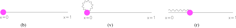
Figure 1: Born (b), virtual (v), and real (r) diagrams for the toy model. The blob represents the system, the wiggly line the emitted photon.

depicted in fig. 1. We write the corresponding contributions to the cross section as follows:

$$\left(\frac{d\sigma}{dx}\right)_{\scriptscriptstyle B} = B\delta(x),$$ (2)

$$\left(\frac{d\sigma}{dx}\right)_{\scriptscriptstyle V} = a\left(\frac{B}{2\epsilon}+V\right)\delta(x),$$ (3)

$$\left(\frac{d\sigma}{dx}\right)_{\scriptscriptstyle R} = a\frac{R(x)}{x},$$ (4)

for the Born, virtual, and real contributions respectively, where $a$ is the coupling constant, $B$ and $V$ are constant with respect to $x$, and

$$\lim_{x\to 0}R(x)=B.$$ (5)

The constant $B$ appears in eqs. (3) and (5) since we expect the residue of the leading singularity of the virtual and real contributions to be given by the Born term times a suitable kernel. (We are cheating a bit here, since we didn’t write the Lagrangian of the toy model from which this property should be derived. We assume it, since it holds in QCD). We take this kernel equal to 1, since this simplifies the computations and it is not restrictive. Finally, $\epsilon$ is the parameter entering dimensional regularization in $4-2\epsilon$ dimensions.

The task of predicting an observable $O$ to NLO accuracy amounts to computing the following integral

$$\left\langle O\right\rangle=\lim_{\epsilon\to 0}\int_{0}^{1}dx\,x^{-2\epsilon}O(x)\left[\left(\frac{d\sigma}{dx}\right)_{\scriptscriptstyle B}+\left(\frac{d\sigma}{dx}\right)_{\scriptscriptstyle V}+\left(\frac{d\sigma}{dx}\right)_{\scriptscriptstyle R}\right],$$ (6)

where $O(x)$ is the observable as a function of $x$, possibly times a set of $\Theta$ functions defining a histogram bin. The condition that the integral of eq. (6) exists is equivalent to the requirement that

$$\lim_{x\to 0}O(x)=O(0).$$ (7)

The analogue of this condition in QCD is known as infrared safety. The main technical problem in eq. (6) is due to the presence of the regularising parameter $\epsilon$. In order to have an efficient numerical procedure, it is mandatory to extract the pole in $\epsilon$ from the real contribution, thus cancelling analytically the pole explicitly present in the virtual contribution. One has to keep in mind that the integral in eq. (6) cannot be fully computed analytically, because of the complicated form of $O(x)$ and $R(x)$.

Two strategies can be devised to solve this problem. In the slicing method, a small parameter $\delta$ is introduced into the real contribution (third term on the r.h.s. of eq. (6)) in the following way:

$$\left\langle O\right\rangle_{\scriptscriptstyle R}=\int_{0}^{\delta}dx\,x^{-2\epsilon}O(x)\left(\frac{d\sigma}{dx}\right)_{\scriptscriptstyle R}+\int_{\delta}^{1}dx\,x^{-2\epsilon}O(x)\left(\frac{d\sigma}{dx}\right)_{\scriptscriptstyle R}.$$ (8)

In the first term on the r.h.s. of this equation we expand $O(x)$ and $R(x)$ in Taylor series around 0 and keep only the first term; the smaller $\delta$, the better the approximation. On the other hand, the second term in eq. (8) does not contain any singularity and we can just set $\epsilon=0$ there. We obtain

$$\left\langle O\right\rangle_{\scriptscriptstyle R} = aBO(0)\int_{0}^{\delta}dx\,\frac{x^{-2\epsilon}}{x}+\int_{\delta}^{1}dx\,O(x)\left(\frac{d\sigma}{dx}\right)_{\scriptscriptstyle R}+{\cal O}(\delta)$$ (9)

$$= a\left(-\frac{1}{2\epsilon}+\log\delta\right)BO(0)+a\int_{\delta}^{1}dx\,\frac{O(x)R(x)}{x}+{\cal O}(\delta,\epsilon).$$ (10)

Using this result in eq. (6), we get the NLO prediction for $\left\langle O\right\rangle$ as given in the slicing method:

$$\left\langle O\right\rangle_{\scriptscriptstyle slice}=BO(0)+a\left[\left(B\log\delta+V\right)O(0)+\int_{\delta}^{1}dx\,\frac{O(x)R(x)}{x}\right]+{\cal O}(\delta).$$ (11)

The terms collectively denoted by ${\cal O}(\delta)$, although computable, can be neglected by choosing $\delta$ small. In practical computations, the integral is performed numerically, but due to the divergence of the integrand for $x\to 0$, $\delta$ cannot be taken too small because of the loss of accuracy of the numerical integration. Thus, the value of $\delta$ is a compromise between these two opposite requirements, being neither too small nor too large. Of course, “small” and “large” are meaningful only when referred to a specific computation. Therefore, when using the slicing method, it is mandatory to check that the physical results are stable against the variation of the value of $\delta$, chosen over a suitable range. In principle, this check would have to be performed for each observable, $O$, computed. In practice, only one observable is considered which is generally chosen to be rather inclusive (such as a total rate).

In the subtraction method, no approximation is performed. One writes the real contribution as follows:

$$\left\langle O\right\rangle_{\scriptscriptstyle R}=aBO(0)\int_{0}^{1}dx\,\frac{x^{-2\epsilon}\Theta(x_{c}-x)}{x}+a\int_{0}^{1}dx\,\frac{O(x)R(x)-BO(0)\Theta(x_{c}-x)}{x^{1+2\epsilon}}\;,$$ (12)

where $x_{c}$ is an arbitrary parameter $0<x_{c}\leq 1$. The second term on the r.h.s. does not contain singularities and we can set $\epsilon=0$ there:

$$\left\langle O\right\rangle_{\scriptscriptstyle R}=-aB\frac{x_{c}^{-2\epsilon}}{2\epsilon}O(0)+a\int_{0}^{1}dx\,\frac{O(x)R(x)-BO(0)\Theta(x_{c}-x)}{x}\;.$$ (13)

Therefore, the NLO prediction as given in the subtraction method is:

$$\left\langle O\right\rangle_{\scriptscriptstyle sub}=BO(0)+a\left[(B\log x_{c}+V)O(0)+\int_{0}^{1}dx\,\frac{O(x)R(x)-BO(0)\Theta(x_{c}-x)}{x}\right].$$ (14)

This equation has to be compared with eq. (11). Although the two are quite similar, there are two important differences that have to be stressed. First, the parameter $x_{c}$ introduced in the subtraction method does not need to be small. (Actually, in the original formulation of the method $x_{c}$ was not even introduced, which corresponds to setting $x_{c}=1$ here). This is due to the fact that in the subtraction method no approximation has been performed in the intermediate steps of the computation. This in turn implies the second point; there is no need to check that the physical results are independent of the value of $x_{c}$, since this is true by construction.

We stress that both eqs. (11) and (14) are quite powerful. The cancellation of the divergent terms, which arise in the intermediate steps of the computation from loop and phase-space integrals for the case of virtual and real contributions respectively, has been achieved without knowing anything about: 1) the observable $O$, apart from its infrared safety, and 2) the matrix elements, apart from their leading singular behaviour (see eq. (5)).

We now turn to the case of QCD. As anticipated, for the time being we assume the world to be made of quarks and gluons, and we compute cross sections for their scatterings. As in the toy model, NLO corrections imply the computation of virtual and real diagrams. According to the toy model, in order to achieve the cancellation of the singularities it is crucial to single out the singular terms in the matrix elements. Let us first consider the case of real emissions. It is not difficult to realise that the only diagrams which can contribute a singularity in the matrix elements are those in which an emission occurs on an external leg (strictly speaking, this is true only in physical gauges). The final-state emission from a quark (the case of emission from a gluon is completely analogous)

Figure 2: Gluon emission from a final-state quark. The blob represents the rest of the diagram.

can be formally represented as in fig. 2. The blob represents the rest of the diagram, which doesn’t play any role in what follows and can be arbitrarily complicated. For the computation of this diagram it is convenient to parametrise the momenta as follows:

$$k_{b}=zk_{a}+k_{\scriptscriptstyle T}+\zeta_{b}n\,,\;\;\;\;\;\;k_{c}=(1-z)k_{a}-k_{\scriptscriptstyle T}+\zeta_{c}n\,,$$ (15)

where $k_{\scriptscriptstyle T}\cdot k_{a}=k_{\scriptscriptstyle T}\cdot n=0$, $n^{2}=0$, $k_{a}^{2}=0$, $n\cdot k_{a}\neq 0$, and the coefficients $\zeta_{b}$, $\zeta_{c}$ are determined by imposing the on-shell conditions

$$k_{b}^{2}=0\;\Rightarrow\;\zeta_{b}=-\frac{k_{\scriptscriptstyle T}^{2}}{2zn\cdot k_{a}}\,,\;\;\;\;\;\;k_{c}^{2}=0\;\Rightarrow\;\zeta_{c}=-\frac{k_{\scriptscriptstyle T}^{2}}{2(1-z)n\cdot k_{a}}\,.$$ (16)

The computation of the diagram is pretty straightforward and tedious so we’ll only report the final result. The contribution to the production cross section is

$$d\sigma^{(1,R)}=\frac{\alpha_{\scriptscriptstyle S}}{2\pi}\int dk_{\scriptscriptstyle T}^{2}dz\,C_{\scriptscriptstyle F}\frac{1+z^{2}}{1-z}\frac{1}{k_{\scriptscriptstyle T}^{2}}d\sigma^{(0)}(k_{a})+{\cal R}.$$ (17)

with the colour factor $C_{\scriptscriptstyle F}=(N_{c}^{2}-1)/(2N_{c})\equiv 4/3$. A regularization prescription is understood in the first term on the r.h.s. of eq. (17). The dimensional regularization adopted in the toy model would imply an extra factor $k_{\scriptscriptstyle T}^{-2\epsilon}(1-z)^{-2\epsilon}$. Alternatively, the singular regions $k_{\scriptscriptstyle T}\sim 0$, $z\sim 1$ could be cut off by computing the integral for $k_{\scriptscriptstyle T}>\mu_{0}$ and $z<1-z_{0}$. The quantity $d\sigma^{(0)}(k_{a})$ is the cross section computed as if the outgoing quark $a$ wouldn’t have split into $b+c$. Pictorially, it corresponds to the square of the black blob, times phase space and normalization factors. ${\cal R}$ denotes all the terms that are not singular in $1/k_{\scriptscriptstyle T}$. $d\sigma^{(1,R)}$ is the analogue of eq. (4) in the toy model, where $x$ plays the role of $k_{\scriptscriptstyle T}$, and $B$ plays the role of $d\sigma^{(0)}$. In the toy model, we would have ${\cal R}=a(R(x)-B)/x$ as a non-singular quantity thanks to eq. (5). Clearly, the structure of eq. (17) is more involved than that of eq. (4) since QCD is more complicated than the toy model. In particular, we see that $d\sigma^{(1,R)}$ is singular not only for $k_{\scriptscriptstyle T}\to 0$ but also for $z\to 1$. These two limits correspond to the emitted quark and gluon being collinear, and to the emitted gluon being soft, respectively. By explicit computation one thus recovers a well known fact of QCD, that matrix elements are singular when two on-shell partons become collinear, or a gluon becomes soft.

If QCD works as the toy model, we expect that, upon regulating the integral appearing in eq. (17), the singularities will cancel against those obtained from the virtual contribution. This is in fact what happens. The loop integrals can easily be cast in the same form as the integral in eq. (17):

$$d\sigma^{(1,V)}=-\frac{\alpha_{\scriptscriptstyle S}}{2\pi}\int dk_{\scriptscriptstyle T}^{2}dz\,C_{\scriptscriptstyle F}\frac{1+z^{2}}{1-z}\frac{1}{k_{\scriptscriptstyle T}^{2}}d\sigma^{(0)}(k_{a})+{\cal V}.$$ (18)

This corresponds to writing $\delta(x)/(2\epsilon)=-\int_{0}^{1}dxx^{-1-2\epsilon}+{\cal O}(\epsilon)$ in the toy model and replacing this expression into eq. (3). The sum of eqs. (17) and (18) is indeed non singular.

We stress that $d\sigma^{(1,R)}+d\sigma^{(1,V)}$ being finite is not the analogue of eq. (11) or eq. (14). In fact, here we limited ourselves to computing the most inclusive of the observables in the kinematics of partons $b$ and $c$, which corresponds to taking $O\equiv 1$ in the toy model. We shall come back later to the treatment of non-trivial observables in the case of QCD. Before doing that, we first have to consider the case in which a splitting occurs in the initial state. The situation is depicted in fig. 3.

Figure 3: Gluon emission from an initial-state quark. The blob represents the rest of the diagram.

The kinematics for this splitting can be again parametrized as in eq. (15). The crucial difference is the momentum entering the blob, being in this case $k_{a}-k_{c}$. The analogue of eq. (17) is

$$d\sigma^{(1,R)}=\frac{\alpha_{\scriptscriptstyle S}}{2\pi}\int dk_{\scriptscriptstyle T}^{2}dz\,C_{\scriptscriptstyle F}\frac{1+z^{2}}{1-z}\frac{1}{k_{\scriptscriptstyle T}^{2}}d\sigma^{(0)}(zk_{a})+{\cal R}.$$ (19)

On the other hand, the kinematics of the virtual term are identical to those relevant to final-state emission (and in fact it is improper to talk about initial- and final-state contributions to the virtual term). Therefore

$$d\sigma^{(1,R)}+d\sigma^{(1,V)}=\frac{\alpha_{\scriptscriptstyle S}}{2\pi}\int dk_{\scriptscriptstyle T}^{2}dz\,C_{\scriptscriptstyle F}\frac{1+z^{2}}{1-z}\frac{1}{k_{\scriptscriptstyle T}^{2}}\left(d\sigma^{(0)}(zk_{a})-d\sigma^{(0)}(k_{a})\right)+{\cal R}+{\cal V}.$$ (20)

This expression is non-singular in the soft limit $z\to 1$, but it is still divergent in the collinear limit $k_{\scriptscriptstyle T}\to 0$. We, therefore, have to conclude that the NLO cross section for a process involving quarks in the initial state is a divergent quantity (the same holds true in the case of gluons in the initial state).

The problem is not as serious as it may seem. To understand this, we have to go back to the real world where no one has, or ever ever will, succeeded in preparing quark or gluon beams. Before QCD was born, Feynman proposed the parton model to describe lepton-hadron collisions. The cross section for the process $e+H\to X$, $X$ being a generic final state, is written as

$$d\sigma(K_{e},K_{H})=\sum_{i}\int_{0}^{1}dyf^{(H)}_{i}(y)d\sigma_{i}(K_{e},yK_{H})\,.$$ (21)

Here, $K_{e}$ and $K_{H}$ are the electron and hadron momenta respectively. The hadron is thought of as a beam of free massless constituents–the partons–which have only longitudinal (with respect to the hadron direction of motion) degrees of freedom. There may be different parton types, which are summed over in eq. (21). The cross section $\sigma_{i}$ is relevant to the process $e+p_{i}\to X$, with $p_{i}$ being a parton of type $i$. Finally, the quantity $dyf^{(H)}_{i}(y)$ is the probability of finding the parton $p_{i}$ with 3-momentum $\vec{k}_{i}$ such that $y\vec{K}_{H}<\vec{k}_{i}<(y+dy)\vec{K}_{H}$. The functions $f^{(H)}_{i}(y)$ are the parton densities (also called parton distribution functions). They describe a property of the partons as hadron constituents and, as such, are independent of the nature of the interactions between the partons and the lepton. This property is called universality.

In QCD, it appears natural to identify the partons with quarks and gluons. The question is: can we compute NLO QCD corrections to $d\sigma_{i}$ in eq. (21)? From eq. (20) we know that the answer is negative, so the parton model does not survive radiative corrections. However, we shall now show that, by suitably modifying it, an equation analogous to eq. (21) holds, with all the quantities appearing in it free of divergences. In order to proceed, we simplify the notation as follows. We assume that the sum in eq. (21) runs only over quarks so we suppress it and its dependence upon $i$. We also suppress writing the dependence upon $K_{e}$ and shorten the notation in eq. (20) by introducing the quantity

$$P(z)=C_{\scriptscriptstyle F}\left(\frac{1+z^{2}}{1-z}\right)_{+}.$$ (22)

This notation is denoted as the “plus prescription” and is defined as follows:

$$\int_{0}^{1}dzh(z)(g(z))_{+}=\int_{0}^{1}dz(h(z)-h(1))g(z)\,.$$ (23)

Thus, neglecting the finite terms ${\cal R}$ and ${\cal V}$, we get

$$d\sigma^{(1,R)}(k_{a})+d\sigma^{(1,V)}(k_{a})=\frac{\alpha_{\scriptscriptstyle S}}{2\pi}\int\frac{dk_{\scriptscriptstyle T}^{2}}{k_{\scriptscriptstyle T}^{2}}dzP(z)d\sigma^{(0)}(zk_{a}).$$ (24)

We can now compute the $k_{\scriptscriptstyle T}^{2}$ integral by cutting off the $k_{\scriptscriptstyle T}\sim 0$ region (so we don’t use dimensional regularization here):

$$\int\frac{dk_{\scriptscriptstyle T}^{2}}{k_{\scriptscriptstyle T}^{2}}\;\longrightarrow\;\int_{\mu_{0}^{2}}^{Q^{2}}\frac{dk_{\scriptscriptstyle T}^{2}}{k_{\scriptscriptstyle T}^{2}}=\log\frac{Q^{2}}{\mu_{0}^{2}}\,,$$ (25)

where $\mu_{0}$ is an arbitrary mass scale with $\mu_{0}\ll Q$, and $Q$ is a characteristic (hard) scale of the process. Thus, the NLO contribution to eq. (21) is

$$d\sigma^{(1)}(K_{H})=\frac{\alpha_{\scriptscriptstyle S}}{2\pi}\log\frac{Q^{2}}{\mu_{0}^{2}}\int dydzf^{(H)}(y)P(z)d\sigma^{(0)}(yzK_{H}).$$ (26)

Since the leading order contribution is

$$d\sigma^{(0)}(K_{H})=\int dyf^{(H)}(y)d\sigma^{(0)}(yK_{H}),$$ (27)

after some simple algebra the full NLO prediction can be cast in the following form (neglecting terms of order $\alpha_{\scriptscriptstyle S}^{2}$), with $\mu_{0}\ll\mu\sim Q$

$$d\sigma(K_{H})=\int dy\hat{f}^{(H)}(y,\mu^{2},\mu_{0}^{2})d\hat{\sigma}(yK_{H},\mu^{2},Q^{2}),$$ (28)

where

$$\hat{f}^{(H)}(y,\mu^{2},\mu_{0}^{2}) = f^{(H)}(y)+\frac{\alpha_{\scriptscriptstyle S}}{2\pi}\log\frac{\mu^{2}}{\mu_{0}^{2}}\int_{y}^{1}\frac{dz}{z}P(z)f^{(H)}(y/z)\,,$$ (29)

$$d\hat{\sigma}(K,\mu^{2},Q^{2}) = d\sigma^{(0)}(K)+\frac{\alpha_{\scriptscriptstyle S}}{2\pi}\log\frac{Q^{2}}{\mu^{2}}\int_{0}^{1}dzP(z)d\sigma^{(0)}(zK).$$ (30)

Eq. (28) is meant to replace eq. (21). As can be seen from eq. (30), the cross section $d\hat{\sigma}$ is finite when removing the cutoff, $\mu_{0}\to 0$, at variance with eq. (20). However, the cutoff dependence has simply been moved from the parton cross section to the parton density $\hat{f}$ , which also acquired in the procedure a dependence on the scale $\mu$. This is quite an achievement. In fact, the cutoff dependence is now universal, in the sense that it does not depend upon the nature of the parton scattering $e+q\to X$. This means that $\hat{f}$ has the same universality characteristic of the $f$ originally introduced in the parton model. Furthermore, the result in eq. (30) is likely to be a good approximation of the all-order result, since the dependence on large scales only implies that the coefficient of $\alpha_{\scriptscriptstyle S}\equiv\alpha_{\scriptscriptstyle S}(\mu)$ is a small number. On the other hand, the same is not true in eq. (29), since the coefficient of $\alpha_{\scriptscriptstyle S}$ is a large number, $\log\mu^{2}/\mu_{0}^{2}$. Thus, an all-order computation of $\hat{f}$ would be necessary in order to obtain a reliable prediction. This is beyond our current capabilities (although progress is being made in lattice computations). However, if we give up the possibility of computing $\hat{f}$, we may assume we can measure it in a given process and use it to predict the cross section of some other process. This will work because of the universality of $\hat{f}$.

Eq. (30) may appear odd because the information on the production process in the ${\cal O}(\alpha_{\scriptscriptstyle S})$ term is entirely contained in $d\sigma^{(0)}$, which is of ${\cal O}(\alpha_{\scriptscriptstyle S}^{0})$. This is because we have neglected in the derivation the finite terms ${\cal R}$ and ${\cal V}$, which should be added on the r.h.s. of eq. (30) to reinstate the correct notation. It is however important to note that the cancellation of the divergences proceeds independently of ${\cal R}$ and ${\cal V}$. The computation of these finite terms, which is the toughest part of any matrix element computation, can be forgotten when dealing with the singularities.

There is possibly a logical flaw in this reasoning, since we didn’t prove that eq. (28) holds to all orders. In fact, this is a highly non-trivial proof, which has been carried out for a number of different processes, such as lepton-hadron and hadron-hadron collisions. The resulting forms, eq. (28) or

$$d\sigma(K_{H_{1}},K_{H_{2}})=\int dy_{1}dy_{2}\hat{f}^{(H_{1})}(y_{1})\hat{f}^{(H_{2})}(y_{2})d\hat{\sigma}(y_{1}K_{H_{1}},y_{2}K_{H_{2}})$$ (31)

for the collisions of hadrons $H_{1}$ and $H_{2}$ with momenta $K_{1}$ and $K_{2}$ respectively go under the name of factorization theorems.

There are a couple of interesting features of the parton densities $\hat{f}$ that deserve some consideration. First, we consider eq. (29), by deriving both sides of the equation with respect to $\log\mu^{2}$, we get

$$\frac{\partial\hat{f}^{(H)}(y,\mu^{2},\mu_{0}^{2})}{\partial\log\mu^{2}}=\frac{\alpha_{\scriptscriptstyle S}}{2\pi}\int_{y}^{1}\frac{dz}{z}P(z)\hat{f}(y/z,\mu^{2},\mu_{0}^{2})+{\cal O}(\alpha_{\scriptscriptstyle S}^{2}).$$ (32)

In this equation, the dependence upon $\mu_{0}$ is entirely contained in $\hat{f}$. Thus, it is sensible to assume the r.h.s. to be the first term of a well-behaved perturbative expansion (in the sense that the next terms will be smaller than this). Eq. (32) is nothing but the familiar Altarelli-Parisi equation (for the non-singlet case), often referred to as the Dokshitzer-Gribov-Lipatov-Altarelli-Parisi (DGLAP) equation.

We can also go back to eq. (26) and wonder what would have happened if we had replaced $\mu_{0}$ with $\mu_{1}\sim\mu_{0}$. Clearly

$$\hat{f}^{(H)}(y,\mu^{2},\mu_{0}^{2})-\hat{f}^{(H)}(y,\mu^{2},\mu_{1}^{2})=\frac{\alpha_{\scriptscriptstyle S}}{2\pi}\log\frac{\mu_{1}^{2}}{\mu_{0}^{2}}\int_{y}^{1}\frac{dz}{z}P(z)f^{(H)}(y/z)\,.$$ (33)

The r.h.s. of this equation is a small number. This suggests that the quantities appearing in eq. (28) could have actually been defined as follows

$$\hat{f}^{(H)}(y,\mu^{2},\mu_{0}^{2},{\cal H}) = f^{(H)}(y)+\frac{\alpha_{\scriptscriptstyle S}}{2\pi}\int_{y}^{1}\frac{dz}{z}\left(\log\frac{\mu^{2}}{\mu_{0}^{2}}P(z)+{\cal H}(z)\right)f^{(H)}(y/z)\,,$$ (34)

$$d\hat{\sigma}(K,\mu^{2},Q^{2},{\cal H}) = d\sigma^{(0)}(K)+\frac{\alpha_{\scriptscriptstyle S}}{2\pi}\int_{0}^{1}dz\left(\log\frac{Q^{2}}{\mu^{2}}P(z)-{\cal H}(z)\right)d\sigma^{(0)}(zK).$$ (35)

The function ${\cal H}(z)$ is largely arbitrary, but the idea is that its contribution to eq. (34) is a small number compared to $\log\mu^{2}/\mu_{0}^{2}$. It should be clear that the dependence of $\hat{f}$ upon ${\cal H}(z)$ is completely different from that upon $\mu_{0}$; ${\cal H}(z)$ is arbitrary, and can be freely changed without changing the l.h.s. of eq. (28). On the other hand, we cannot control the dependence upon $\mu_{0}$, which is fixed by Nature. For this reason, it is customary to suppress writing it in the arguments of $\hat{f}$. It should therefore be clear that neither $\hat{f}$ nor $d\hat{\sigma}$ are physical quantities, since they depend on our conventions. Still, with a given choice of ${\cal H}(z)$, $\hat{f}$ is universal and can therefore be used in the computation of eq. (31), provided that $d\hat{\sigma}$ there is defined according to the same conventions used in eq. (35). The choice of ${\cal H}(z)$ is usually denoted as scheme choice, with popular schemes, such as ${\rm\overline{MS}}$ or DIS, using a specific form for ${\cal H}(z)$. We stress again that not only parton densities, but also parton cross sections are computed in a given scheme. An error, of next-to-leading order, is made if one predicts an observable using parton densities and parton cross sections computed in different schemes. Therefore, standard Monte Carlo parton shower codes, which implement hard cross sections only at the leading order, can be used with parton densities defined in whatever scheme. On the other hand, care is required with codes that implement NLO corrections, since the parton density scheme must match that used in the parton cross sections.

In summary, with a purely theoretical argument (the presence of collinear divergences in the cross section for a process involving quarks in the initial state) we showed that a world without hadrons cannot exist (or at least that QCD is not able to describe it). The parton model doesn’t survive radiative corrections. However, its analogue in perturbative QCD, the factorization theorem, is based on the very same physical picture. Although hadrons, and not quarks and gluons, are present in the final state, no final-state collinear divergences are found in the cross section we previously computed. This is at variance with eq. (20), where the sum of eqs. (17) and (18) is finite. This prevents us from using quantities akin to parton densities in the final state, which would convert quarks and gluons into the observed hadrons (since we have explicitly shown that the introduction of parton densities is associated with the presence of collinear divergences). In order to give a physical meaning to QCD computations, one has to assume that those cross sections which can be computed in terms of quarks and gluons, and are free of infrared and collinear divergences, correspond to cross sections of physical hadrons. This assumption is know as hadron-parton duality. For example, the computation at ${\cal O}(\alpha_{\scriptscriptstyle S}^{n})$ of the total rate for producing any number of quarks and gluons in $e^{+}e^{-}$ collisions has to be interpreted as the ${\cal O}(\alpha_{\scriptscriptstyle S}^{n})$ prediction for the total $e^{+}e^{-}$ hadronic cross section.

It is not difficult to obtain a QCD cross section with final-state collinear divergences. For example, this would have happened by fixing the momentum of the gluon $c$ in fig. 2. In general, the final-state quark and gluon momenta are combined in order to define the observable we want to study. In the previous example, we considered the simplest possible observable, the total rate, which corresponds to setting $O(x)\equiv 1$ in the toy model. In general, the observable definition in terms of momenta is non trivial. Since the kinematics of the real and virtual diagrams are different, so is the definition of the observable. In the toy model, the contribution of the real (virtual) diagrams to the observable $O$ is $O(x)$ ($O(0)$), and the condition of eq. (7) must be fulfilled in order to obtain a finite cross section. Physically, the meaning of eq. (7) is clear; the smaller the emitted photon energy, the closer the value of the observable to the value of the observable computed when no emissions have occurred. It is easy to prove that analogous conditions must hold in QCD for avoiding divergences: the observable value must be insensitive to soft emissions or collinear splittings. These conditions are known as infrared safety.

With an infrared-safe jet definition, hadron-parton duality is the understood assumption in the extremely successful comparisons between jet data and NLO parton-level computations. On the other hand, there are physically interesting cases associated with final-state collinear divergent QCD cross sections (for example, $\pi^{0}$ spectra in $p\bar{p}$ collisions). In these cases, the day is saved by applying parton-model techniques to final-state emissions, that is, by proving other factorization theorems. The cross section is written analogously to eq. (28)

$$d\sigma(K_{H})=\int dzd\hat{\sigma}_{a}(K_{H}/z,\mu^{2},Q^{2})\hat{D}^{(a)}_{H}(z,\mu^{2},\mu_{0}^{2}),$$ (36)

where $K_{H}$ is now the momentum of the final-state hadron $H$, $d\hat{\sigma}_{a}$ is the cross section for producing a final-state parton $a$, and $\hat{D}^{(a)}_{H}$ is analogous to $\hat{f}^{(H)}$, which is related to the probability density of finding a hadron $H$ within a parton $a$, rather than to the probability of finding a parton in a hadron. This “final-state parton density” is actually a hadron density and is called a fragmentation function. In eq. (36) all the quantities are finite, with those on the r.h.s. being defined through equations similar to eqs. (29) and (30). Notice that the finiteness of eq. (36) is not in contradiction with what was said before. In fact, the fragmentation functions cannot be computed in perturbation theory. However, similarly to the parton densities, they can be extracted from data in an universal manner, i.e. independently of the collision process considered.

It is worth mentioning that the factorization theorems and the hadron-parton duality hold up to terms proportional to some inverse power of the hard scale of the process, $1/Q^{p}$. For this reason, these terms are usually referred to as power-suppressed terms. In real experiments, the scale $Q$ may not be large enough for them to be safely neglected in the comparison with perturbative QCD predictions. In the vast majority of cases, they are estimated with the help of parton shower Monte Carlos, although alternative approaches exist for $e^{+}e^{-}$ and $eH$ collisions.

The factorization theorems and the hadron-parton duality are a rather powerful machinery, and allow the computation of QCD corrections to the observable that one wants to compare with data. Nowadays, NLO predictions exist for the vast majority of observables measured by experiments and a few NNLO computations are available as well. Because of the delicate singularity cancellations, early computations were typically performed for a specific observable in a given collision process. However, it was later realised that such cancellations basically rely on properties common to all matrix elements and are independent of the observable being studied (apart from the requirement that it be infrared safe). This forms the core of the so-called universal formalisms for dealing with infrared singularities. These formalisms, at present only available at the NLO, allow one to write any cross section in terms of finite quantities, obtained with a well-defined prescription from matrix-element computations (in the example given before, these finite quantities are $d\sigma^{(0)}$, ${\cal R}$, and ${\cal V}$). Barring involved technical details, the resulting expressions are analogous to eqs. (11) or (14). Precisely as in the toy model, popular universal formalisms rely either on the slicing or on the subtraction method. They differ in the way in which the slicing parameters are introduced or in the way in which the subtraction terms are defined.

The universal formalisms can be easily implemented in numerical programs, which compute $\left\langle O\right\rangle$ for any observable $O(x)$. From eqs. (11) and (14), it should be clear that these programs are simply integrators, and the integral is typically computed with Monte Carlo techniques. The word “integrator” is usually understood or forgotten and “Monte Carlo” is what remains. We shall refer to them as Monte Carlo Integrators (MCI) in what follows. The confusion with parton shower Monte Carlos (PSMC) is worsened by the fact that one insists that events are produced by MCI’s, not only by PSMC’s. In order to clarify that the word event is used in MCI’s and PSMC’s with different meanings, consider eq. (14). Let’s pretend that only the last term is present (the remaining ones can be treated similarly) and to simplify the notation set $x_{c}=1$. The procedure to obtain $\left\langle O\right\rangle_{\scriptscriptstyle sub}$ with Monte Carlo techniques can be summarised as follows:

• Pick at random $0\leq x\leq 1$.

• Compute $w_{\scriptscriptstyle EV}=aR(x)/x$ (the event weight).

• Compute $w_{\scriptscriptstyle CT}=-aB/x$ (the counter-event weight).

• Call an output routine, that adds $w_{\scriptscriptstyle EV}$ to the bin to which $O(x)$ belongs and $w_{\scriptscriptstyle CT}$ to the bin to which $O(0)$ belongs.

• Repeat the preceding steps $N$ times and normalise with $1/N$.

Picking $x$ at random is equivalent to generating the configuration $(r)$ in fig. 1. Since this configuration and its corresponding weight $w_{\scriptscriptstyle EV}$ are independent of $O(x)$, one calls it an event. This is similar to what happens in PSMC, where events are generated with no reference to an observable. There is more to this similarity, since the output routine of the fourth step can be called for many different observables for a given event and eventually predict all of them with a single integration procedure. On the other hand, at variance with PSMC’s, each event is accompanied by a counter-event, whose weight is $w_{\scriptscriptstyle CT}$ and whose kinematics corresponds to $(v)$ (or $(b)$, which is equivalent) in fig. 1. Suppose an $x$ value very close to 0 is generated. The quantities $w_{\scriptscriptstyle EV}$ and $w_{\scriptscriptstyle CT}$ will be very large in absolute value and opposite in sign. In fact, because of eq. (5), they are almost identical, up to the sign. Thus, if $O(x)$ and $O(0)$ fall in the same bin, the contributions of the event and of the counter-event tend to cancel and only a small leftover will contribute to that bin. If, on the other hand, $O(x)$ and $O(0)$ belong to different bins, the cross section in these bins will be extremely large in absolute value. Notice that this can happen also if $O$ is infrared safe, i.e. it fulfils the condition of eq. (7), so it is sufficient to chose a very small bin size. One typically says that QCD does not have infinite-resolution power. Finally, let’s try to use our MCI as an unweighted-event generator. According to the hit-and-miss technique (see sect. 2), preliminarily one needs to estimate the maximum of the weight distribution. Since $w_{\scriptscriptstyle EV}$ is divergent for $x\to 0$, the unweighting procedure is simply undefined. This problem can be circumvented by introducing a small cutoff (such as $\delta$ of the slicing method), where the maximum weight will then be $\sim aB/\delta$. However, the smaller $\delta$, the less efficient the unweighting procedure. In summary, an MCI is an event generator is the sense that: a) the word events implies events and counter-events, as defined above; b) only weighted events can be generated and the weights may have positive or negative values, the latter being typically associated with counter-events; c) the events consist of a few final-state quarks and gluons (i.e., not hadrons).

5 PARTON DISTRIBUTION FUNCTIONS 

As pointed out in sect. 4, the calculation of any production cross sections relies upon a knowledge of the distribution of the momentum fraction $x$ of the partons (quarks and gluons) in the incoming hadrons in the relevant kinematic range. These parton densities or parton distribution functions (PDF’s) can not be calculated perturbatively but rather are determined by global fits to data from deep inelastic scattering (DIS), Drell-Yan (DY), and jet production at current energy ranges. Two major groups, CTEQ and MRST, provide semi-regular updates to the parton distributions when new data and/or theoretical developments become available. The newest PDF’s, in most cases, provide the most accurate description of the world’s data, and should be utilised in preference to older PDF sets. The newest sets from the two groups are CTEQ6.1 [106] and MRST2002 [82].

Processes Involved in Global Analysis Fits

Measurements of DIS structure functions ($F_{2},F_{3}$) in lepton-hadron scattering and of lepton pair production cross sections in hadron-hadron collisions provide the main source of information on quark distributions $f_{q}^{(p)}(x,Q^{2})$ inside protons. At leading order, the gluon distribution function $f_{g}^{(p)}(x,Q^{2})$ enters directly in hadron-hadron scattering processes with jet final states. Modern global parton distribution fits are carried out to next-to-leading order which allows $\alpha_{\scriptscriptstyle S}(Q^{2})$, $f_{q}^{(p)}(x,Q^{2})$ and $f_{g}^{(p)}(x,Q^{2})$ to all mix and contribute in the theoretical formulae for all processes. Nevertheless, the broad picture described above still holds to some degree in global PDF analyses.

The data from DIS, DY and jet processes utilised in PDF fits cover a wide range in $x$ and $Q$, but need to be extrapolated to cover the range accessible at LHC. HERA data (H1+ZEUS) are predominantly at low $x$, while the fixed target DIS and DY data are at higher $x$. There is considerable overlap, however, with the degree of overlap increasing with time as the statistics of the HERA experiments increases. Parton distributions determined at a given $x$ and $Q^{2}$ ’feed-down’ to lower $x$ values at higher $Q^{2}$ values. DGLAP-based NLO pQCD should provide an accurate description of the data (and of the evolution of the parton distributions) over the entire kinematic range currently accessible. At very low $x$ and $Q$, DGLAP evolution is believed to be no longer applicable and a BFKL description must be used. No clear evidence of BFKL physics is seen in the current range of data; thus all global analyses use conventional DGLAP evolution of PDF’s.

There is a remarkable consistency between the data in the PDF fits and the NLO QCD theory fit to them. On the order of 2000 data points or more are used in modern global PDF analyses and the $\chi^{2}$/DOF for the fit of theory to data is on the order of 1.

The accuracy of the extrapolation to higher $Q^{2}$ depends on the accuracy of the original measurement, any uncertainty on $\alpha_{\scriptscriptstyle S}(Q^{2})$ and the accuracy of the evolution code. Current programs in use by CTEQ and MRST should be able to carry out the evolution using NLO DGLAP to an accuracy of a few percent over the hadron collider kinematic range, except perhaps at very large $x$ and very small $x$. Evolution programs are also currently available which use approximate expressions for NNLO Altarelli-Parisi kernels.

Parameterizations and Schemes

A global PDF analysis carried out at next-to-leading order needs to be performed in a specific renormalization and factorization scheme. The evolution kernels are in a specific scheme, and to maintain consistency any hard scattering cross section calculations used for the input processes or utilising the resulting PDF’s need to have been implemented in that same scheme (see sect. 4). Almost universally, the $\overline{\mathrm{MS}}$ scheme is used, but PDF’s are also available in the DIS scheme, a fixed flavour scheme, and several schemes that differ in their specific treatment of the charm quark mass.

Some global analyses have also been carried out at NNLO [83, 4]. However, the NNLO evolution kernels are still known only approximately and only the DIS cross sections are known to NNLO. The other cross sections are still treated at NLO.

It is also possible to use only leading-order matrix element calculations in the global fits which results in leading-order parton distribution functions. Such PDF’s are the standard choice when leading order matrix element calculations (such as Monte Carlo programs like Herwig and Pythia) are used. The differences between LO and NLO PDF’s, though, are formally NLO. Thus, the additional error introduced by using a NLO PDF with Herwig, rather than a LO PDF, should not be significant, in principle, and NLO PDF’s can be used when no LO alternatives are available (see sect. 4 for a discussion on this point). The differences between NLO and LO parton distributions are not that large for many PDF’s in many regions of $x$ and tend to shrink at higher $Q^{2}$.

All global analyses use a generic form for the parameterization of both the quark and gluon distributions at some reference value $Q_{o}$:

$$F(x,Q_{o})=A_{o}x^{A_{1}}(1-x)^{A_{2}}P(x;A_{3},...)\,.$$ (37)

The reference value $Q_{o}$ is usually chosen in the range of 1-2 GeV. The parameter $A_{1}$ is associated with small-$x$ Regge behaviour, while $A_{2}$ is associated with large-$x$ valence counting rules. In general, the first two factors are not sufficient to describe either quark or gluon distributions. The term $P(x;A_{3},...)$ is a suitably chosen smooth function, depending on one or more parameters, that adds more flexibility to the PDF parameterization. In general, both the number of free parameters and the functional form can have an influence on the global fit.

The PDF’s made available to the world from the global analysis groups can either be in a form where the $x$ and $Q^{2}$ dependence is parameterised or the PDF’s for a given $x$ and $Q^{2}$ range can be interpolated from either a grid which is provided or can be generated given the starting parameters for the PDF’s (see the discussion on LHAPDF given below). All of these techniques should provide an accuracy on the output PDF distributions of the order of a few percent.

The parton distributions from the recent CTEQ PDF release are plotted in Figure 4 at a $Q$ value of $100$ GeV. The gluon distribution is dominant at $x$ values of less than .02 with the valence quark distributions dominant at higher $x$.

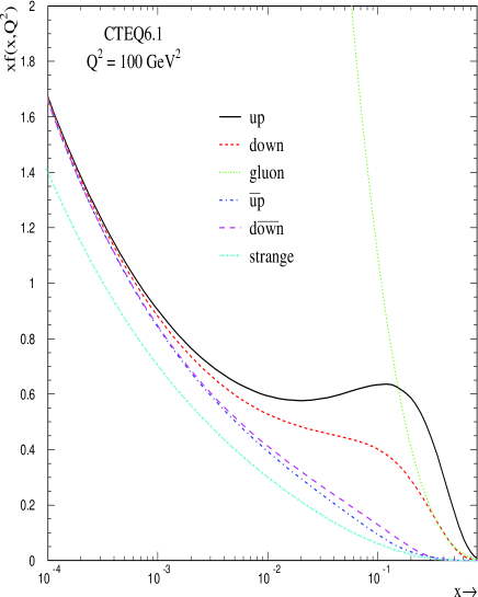
Figure 4: Several PDF’s from the CTEQ6.1 set plotted at a $Q^{2}$ value of 100 $GeV^{2}$.

Uncertainties on PDF’s

In addition to having the best estimates for the values of the PDF’s in a given kinematic range, it is also important to understand the allowed range of variation of the PDF’s, i.e. their uncertainties. A conventional method of estimating parton distribution uncertainties has been to compare different published parton distributions. This is unreliable since most published sets of parton distributions (for example from CTEQ and MRST) adopt similar assumptions and the differences between the sets do not fully explore the uncertainties that actually exist.

The sum of the quark distributions $\left(\Sigma[f_{q}^{(p)}(x,Q)+f_{\overline{q}}^{(p)}(x,Q)]\right)$ is, in general, well-determined over a wide range of $x$ and $Q^{2}$. As stated above, the quark distributions are predominantly determined by the DIS and DY data sets which have large statistics, and systematic errors in the few percent range ($\pm 3\%$ for $10^{-4}<x<0.75$). Thus the sum of the quark distributions is basically known to a similar accuracy. The individual quark flavours, though, may have a greater uncertainty than the sum. This can be important, for example, in predicting distributions that depend on specific quark flavours, like the $W$ rapidity distribution and its asymmetry.

The largest uncertainty of any parton distribution, however, is that on the gluon distribution. The gluon distribution can be determined indirectly at low $x$ by measuring the scaling violations in the quark distributions, but a direct measurement is necessary at moderate to high $x$. The best direct information on the gluon distribution at moderate to high $x$ comes from jet production at the Tevatron.

There has been a great deal of recent activity on the subject of PDF uncertainties. Two techniques in particular, the Lagrange Multiplier and Hessian techniques, have been used by CTEQ and MRST to estimate PDF uncertainties [89, 82]. The Lagrange Multiplier technique is useful for probing the PDF uncertainty of a given process, such as the $W$ cross section, while the Hessian technique provides a more general framework for estimating the PDF uncertainty for any cross section.

In the Hessian method a large matrix (20x20 for CTEQ, 15x15 for MRST), with dimensions equal to the number of free parameters in the fit, has to be diagonalised. The result is 20 (15) orthogonal eigenvector directions for CTEQ (MRST) which provide the basis for the determination of the PDF error for any cross section. The larger eigenvalues correspond to directions which are well-determined. Each PDF error results from an excursion along the “+” and “-” directions for each eigenvector. The excursions are symmetric for the larger eigenvalues, but may be asymmetric for the more poorly determined directions. There are 40 PDF’s for the CTEQ error set and 30 for the MRST error set–one for each eigenvector direction. For a given event, it is necessary to recalculate the event weight for each of the error sets in order to evaluate the PDF uncertainty.

Perhaps the most controversial aspect of PDF uncertainties is the determination of the $\Delta\chi^{2}$ excursion from the central fit that is representative of a reasonable error. CTEQ chooses a $\Delta\chi^{2}$ value of 100 (corresponding to a 90% CL limit) while MRST uses a value of 40. Thus, in general, the PDF uncertainties for any cross section will be larger for the CTEQ set than for the MRST set. Except at high $x$ ($>0.5$), the uncertainties on the $u$-quark and $d$-quark distributions are less than 5%, while the uncertainty on the gluon distribution is less than 10% for $x$ values smaller than 0.2.

LHAPDF

Libraries such as PDFLIB [87] have been established that maintain a large collection of available PDF’s. However, PDFLIB is no longer supported making it more difficult for easy access to the most up-to-date PDF’s. In addition, the determination of the PDF uncertainty of any cross section typically involves the use of a large number of PDF’s (on the order of 30-100) and the manner in which the PDF’s are stored in PDFLIB (grids in $x$ and $Q$) make storage of such ensembles very unwieldy.

At Les Houches in 2001, representatives from a number of PDF groups were present and an interface was defined (Les Houches accord 2, or LHAPDF [49]) that allows the compact storage of the information needed to define a PDF. Each PDF is determined by only a few lines of information (basically the starting values of the parameters at $Q=Q_{o}$) and the interface carries out the evolution to any $x$ and $Q$ value, at either LO or NLO as appropriate for each PDF.

The interface is as easy to use as PDFLIB and consists essentially of 3 subroutine calls:

• call InitPDFset(name): called once at the beginning of the code; name is the file name of the external PDF file that defines the PDF set (for example, CTEQ, GKK [48] or MRST).

• call InitPDF(mem): mem specifies the individual member of the PDF set.

• call evolvePDF(x,Q,f): returns the PDF momentum distributions for flavour f at a momentum fraction x and scale Q.

The interface can be downloaded at durpdg.dur.ac.uk/lhapdf/downloads. It is currently included in the matrix element program MCFM (see mcfm.fnal.gov) and will be included in future versions of the cross section integrators and event generator programs. Recent modifications make it possible to include all error PDF’s in memory at the same time. Such a possibility reduces the amount of time needed for PDF error calculations on any observable.

Resources available

The PDF’s and relevant information can be obtained from the CTEQ and MRST groups at web addresses given in the references. LHAPDF can be downloaded from
http://durpdg.dur.ac.uk/lhapdf. There is also a site where PDF’s (and their uncertainties) can be displayed on-line: http://durpdg.dur.ac.uk/hepdata/pdf3.html.

6 HIGHER ORDER CORRECTIONS – SHOWERING AND HADRONIZATION EVENT GENERATORS 

Programs which employ the parton shower approach, such as PYTHIA, HERWIG, and ISAJET, have enjoyed widespread use by experimentalists. These programs, referred to as showering and hadronization generators (SHG’s), are general purpose tools able to simulate a wide variety of initial and final states. They begin with a leading order hard subprocess such as the one ($u\bar{u}\to d\bar{d}$) described in sect. 2. Higher order effects are added by “evolving” the event using the parton shower, which allows partons to split into pairs of other partons (this splitting is usually denoted as branching in this context). The resultant partons are then grouped together or hadronized into colour-singlet hadrons and resonances are decayed. Finally, the underlying structure of the event is generated: beam remnants, interactions from other partons in the hadrons, and collisions between other hadrons in the colliding beams (called pile-up).

The general structure of the final state of an event from an SHG is shown in Figure 5. The time evolution of the event goes from bottom to top. Two protons (each indicated by three solid lines to denote their valence quark content) collide and a parton is resolved at scale $Q$ and momentum fraction $x$ in each one. The phenomenology of the parton resolution is encoded in the parton distribution function $f(x,Q^{2})$. In this example, a valence quark is resolved in the proton shown on the left, while an anti-quark is resolved from the proton on the right’s sea quark distribution. The quark and anti-quark annihilate into an $s$-channel resonance denoted by a wavy line. The resonance then decays into a fermion anti-fermion pair. This part of the event is called the hard subprocess. If the resonance is a $Z^{0}$ and the initial- and final-state fermion anti-fermion pairs are $u\bar{u}$ and $d\bar{d}$ respectively, the physics described in the hard subprocess is exactly that which is contained in the basic event generator of sect. 2. As briefly outlined there, the SHG incorporates higher order QCD effects by allowing the (anti)quarks to branch into $q\!\!\!\!^{{}^{(-)}}g$ pairs, while the gluons may branch into $q\bar{q}$ or $gg$ pairs. The resultant partons may also branch, resulting in a shower or cascade of partons. This part of the event is labelled parton shower in the figure. Showering of the initial state partons is also included in the SHG’s, but is not shown in the figure for simplicity. The event now consists of a number of elementary particles, including quarks, antiquarks, and gluons which are not allowed to exist in isolation, as dictated by colour confinement. Next, the program groups the coloured partons into colour-singlet composite hadrons using a phenomenological model referred to as hadronization. The hadronization scale is in the non-perturbative regime and the programs use fairly crude phenomenological models, which contain several non-physical parameters that are tuned using experimental data. Nevertheless, since the hadronization scale is much smaller than the hard scale(s), the impact of the hadronization model choice on the final result is typically small for most physical processes. After hadronization, many short-lived resonances will be present and are decayed by the program.

The SHG’s also add in features of the underlying event. The beam remnants are the coloured remains of the proton which are left behind when the parton which participates in the hard subprocess is ‘pulled out’. The motion of the partons inside the proton results in a small ($\approx 1$ GeV) primordial transverse momentum, against which the beam remnants recoil. The beam remnants are colour connected to the hard subprocess and so should be included in the same hadronization system. Multiple parton-parton interactions, wherein more than one pair of partons from the beam protons interact, are also accounted for. In a final step, pile-up from other proton-proton collisions in the same bunch crossing are added to the event.

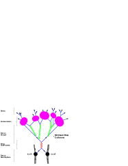
Figure 5: The basic structure of a showering and hadronization generator event is shown schematically[35].

SHG’s produce events with the frequency predicted by theory, so they are event generators in the true sense (as opposed to cross section integrators). One important related point about the generation of an event with the SHG’s is that, with a few minor exceptions, the hard subprocess is the only process dependent part. Everything else is (almost) completely generic and implementing a new physics process usually only involves implementing the computer code for a new hard subprocess. The SHG’s are normally implemented such that the generation of everything except the hard subprocess happens with unit probability—i.e. only the hard subprocess has a weight associated with it. This means (with certain exceptions which are unimportant here) that after selecting a hard subprocess event using the hit-and-miss method (see sect. 2), all the other aspects of the generation are added onto the accepted event without ever rejecting the event. This is important for the modularisation of event generators. Thus when an event generator simulates the hard subprocess a large number of candidate events are attempted, but only a fraction of those candidates are accepted. However, for each hard subprocess event that is chosen and subjected to the subsequent steps of the generation process, one fully simulated event will come out.

Another important aspect of SHG’s is that they provide an exclusive description of the events. As an example, consider the production of a $Z^{0}$ boson as the hard subprocess. As already stressed, at the leading order (i.e., prior to the shower) the transverse momentum of the $Z^{0}$ will always be zero, because there is nothing for the $Z^{0}$ to recoil against. The SHG’s produce transverse momentum for the $Z^{0}$ through the parton shower, since the final-state particles emerging from the hard subprocess must recoil against those produced by the shower, in order to conserve momentum. This prediction of the $Z^{0}$ transverse momentum is termed exclusive because of the detailed listing (the event record) of the particles recoiling against the $Z^{0}$ is provided. In contrast, a cross section integrator results in an inclusive prediction because it generally outputs only the $Z^{0}$ variables and no information about what the $Z^{0}$ is recoiling against is provided. Exclusive calculations—such as those provided by SHG’s—are ideal for the simulation of experiments, because the full event is necessary for detailed detector simulation.

The most important characteristic for SHG’s is the manner in which they treat higher order QCD corrections with the parton shower. As such, this process is described in more detail below. We note that although some “predictions” of the SHG (hadronization, underlying event, etc.) have been used in the past in conjunction with NLO cross section integrators, these procedures have always been heuristic and far from being rigorous. (For example, there is no solid theoretical argument that justifies the procedure of correcting the NLO parton-level predictions for jets to the hadron level, which is usually performed by multiplying the former by the ratio of hadron-level to parton-level cross sections in SHG’s). In particular, the use of the parton shower with NLO matrix elements has, until recently, been “off-limits” due to problems with double counting (essentially the corrections will be applied twice). In sect. 8 we discuss a new class of programs which incorporate NLO matrix elements into SHG’s in a consistent manner.

The Parton Shower 

The parton shower step in Monte Carlo event generation serves two main purposes:

• To provide estimates of higher-order corrections that are enhanced by large kinematic logarithms. These occur in the phase space regions of collinear parton branching and/or soft gluon emission;

• To generate high-multiplicity partonic states which can readily be converted into the observed hadrons by a soft hadronization mechanism, i.e. one that involves only modest transfers of momentum or quantum numbers between neighbouring regions of phase space.

Schematically, the parton shower is a Markov process in which successive values of an evolution variable $t$, a momentum fraction $z$ and an azimuthal angle $\phi$ are generated, together with the flavours of the partons emitted during showering. The evolution variable $t$ starts at some high value $T$, characteristic of the hard process, and the next value is selected by solving the equation

$$\Delta_{i}(T,t_{0})={\cal R}\,\Delta_{i}(t,t_{0})$$ (38)

where $\Delta_{i}$ is the Sudakov form factor for partons of the relevant flavour $i$, $t_{0}$ is an infrared cutoff and ${\cal R}\in[0,1]$ is a random number. The Sudakov form factor is

$$\Delta_{i}(T,t_{0})=\exp\left[-\sum_{j}\int_{t_{0}}^{T}\frac{dt}{t}\int_{0}^{1}dz\,{\cal P}_{ji}(z,t,t_{0})\right]$$ (39)

where ${\cal P}_{ji}$ is the probability distribution for the parton branching $i\to j$. Naively, this is given by $\alpha_{\scriptscriptstyle S}P_{ji}(z)/2\pi$ where $P_{ji}$ is the corresponding DGLAP splitting function. However, in practice the parton branching probabilities are modified in various ways, the details of which depend on the precise definition of the evolution variable and the way in which the shower is implemented:

1. The splitting functions have infrared singularities at $z=0$ and/or 1, which have to be regularised. Normally this is done by cutting out the singular part of the region of integration, in a way that depends on the evolution variable $t$ and the cutoff $t_{0}$. For example, for the splitting $g\to gg$ in HERWIG we have $\sqrt{t_{0}/t}<z<1-\sqrt{t_{0}/t}$ (see below).

2. Quark mass effects may be taken into account in the splittings $q\to qg$ and $g\to q\bar{q}$, leading to splitting functions that depend on quark masses and the evolution variable as well as $z$.

3. The argument of $\alpha_{\scriptscriptstyle S}$ will depend on the evolution scale $t$ and on the momentum fraction $z$, if important higher-order corrections are absorbed into the running of the coupling. The optimal argument, at least in the case of light partons, is the relative transverse momentum generated in the splitting.

4. Other higher-order corrections may be included in the splitting functions. In this case $1\to 3$ parton splittings can also occur; we ignore this possibility in the following discussion.

With all these complications, it is impossible to evaluate the integrals in eq. (39) in closed form and eq. (38) cannot be solved analytically. One can, of course, do numerical integrations and construct look-up tables of the Sudakov form factors, as is done in HERWIG. A neater method, adopted in PYTHIA and Herwig++, is to make use of the rejection method. This involves finding an upper bound ${\cal P}^{\prime}_{ji}>{\cal P}_{ji}$ for which the integrals can be done and the equation solved for the next value, $t^{\prime}$, of the evolution variable. Since the Sudakov form factor with ${\cal P}^{\prime}_{ji}$ in place of ${\cal P}_{ji}$ is a steeper function of $t$, the selected value $t^{\prime}$ will tend to be too high. By accepting this value with probability ${\cal P}_{ji}/{\cal P}^{\prime}_{ji}$, and restarting the evolution with $t^{\prime}$ in the place of $T$ if it is rejected, one can generate the correct distribution quite efficiently without any pre-tabulation.

If several types of branching are available for partons of flavour $i$, for example $g\to q_{j}\bar{q}_{j}$ and $g\to gg$, the next value of the evolution variable can be selected conveniently by treating each type separately and selecting the one that chooses the largest value. This allows the rejection method to be optimised separately for each type of branching.

If the selected value of $t$ is less than the cutoff value $t_{0}$, i.e. if the random number in eq. (38) is ${\cal R}<\Delta_{i}(T,t_{0})$, then the evolution of parton $i$ has finished. It can emit no more (resolvable) partons and is ready to enter the hadronization stage of the generator. Depending on the hadronization model, the parton may be set on mass-shell or given a virtuality of order $t_{0}$.

Otherwise, the next value of the evolution variable $t$ and the type of branching $i\to j$ having been selected, the momentum fraction $z$ of the branching is chosen by solving the equation

$$\int_{0}^{z}\,dz^{\prime}{\cal P}_{ji}(z^{\prime},t,t_{0})={\cal R}^{\prime}\int_{0}^{1}\,dz^{\prime}{\cal P}_{ji}(z^{\prime},t,t_{0})$$ (40)

where ${\cal R}^{\prime}\in[0,1]$ is another random number. Here again a rejection method can be applied, using the upper bound ${\cal P}^{\prime}_{ji}$ on the branching probability distribution.

Knowledge of $t$ and $z$ at each branching allows (almost) complete reconstruction of the kinematics of the parton shower. The details depend on the precise meaning of the shower variables. In PYTHIA, $t$ is the virtuality of the parent parton and $z$ is a light-cone momentum fraction. The relative transverse momentum of the branching (neglecting the virtuality of the daughters) is then given by $q_{t}^{2}=z(1-z)t$. On the other hand, in HERWIG $t$ represents $E^{2}(1-\cos\theta)$ where $E$ is the energy of the parent parton and $\theta$ is the opening angle, while $z$ is an energy fraction, so that $q_{t}^{2}=2z^{2}(1-z)^{2}t$. In either case, we see that the Sudakov form factor (39) incorporates the resummation of leading collinear ($q_{t}^{2}\to 0$) singularities to all orders.

The remaining quantity to be fixed at each branching is the azimuthal angle $\phi$, which fixes the direction of the relative transverse momentum $q_{t}$. This can be chosen with varying degrees of sophistication. The simplest approach is to assume a uniform distribution. More accurately, one can build in the correct azimuthal correlations between successive branchings in the collinear approximation. However, the effect of these is small, since the only branching with a strong azimuthal correlation is the rare gluon splitting, $g\to q\bar{q}$.

Once a branching has occurred, say $i\to jk$ at scale $t_{i}$, the evolution of the daughter partons $j$ and $k$ has to be generated. At the simplest level, their evolution starts at scale $t_{i}$ and the next values $t_{j}$ and $t_{k}$ are obtained from eq. (38) using the appropriate Sudakov form factors $\Delta_{j}$ and $\Delta_{k}$, respectively, with $T$ replaced by $t_{i}$. However, this implies that $t_{j}$ and $t_{k}$ can both be arbitrarily close to $t_{i}$, which is impossible. In PYTHIA, the virtualities of the daughters are constrained by the kinematic relation $\sqrt{t_{j}}+\sqrt{t_{k}}<\sqrt{t_{i}}$. In HERWIG the constraint is even stronger, due to angular ordering. Recall that in HERWIG $t_{i}=E_{i}^{2}(1-\cos\theta_{i})$, where $\theta_{i}$ is the opening angle in the branching $i\to jk$. Angular ordering means that the opening angle $\theta_{j}$ of any subsequent branching of parton $j$ is less than $\theta_{i}$ and, therefore, $t_{j}=E_{j}^{2}(1-\cos\theta_{j})<z^{2}t_{i}$, where $z=E_{j}/E_{i}$. Hence the evolution of parton $j$ starts at $z^{2}t_{i}$ rather than $t_{i}$. Correspondingly, the evolution of parton $k$ starts at $(1-z)^{2}t_{i}$. Note that the condition for further evolution to be possible is that $z^{2}t_{i},(1-z)^{2}t_{i}>t_{0}$, which leads to the condition $\sqrt{t_{0}/t_{i}}<z<1-\sqrt{t_{0}/t_{i}}$ mentioned above. In PYTHIA the angular ordering constraint is applied subsequently using the rejection method, so its relation to the shower variables is not so direct.

Angular ordering represents an attempt to simulate more accurately those higher-order contributions that are enhanced due to soft gluon emission (and associated virtual corrections). A soft gluon emitted by one of the daughter partons in the branching $q\to qg$, for example, can only resolve the individual outgoing quark and gluon colour charges if its angle of emission is less than the opening angle of the branching. Otherwise, it is emitted by the coherent sum of their colour charges, which is equal to that of the parent quark. Therefore we should generate any emission at larger angles from the parent, not the daughters; this corresponds to angular ordering. It leads to a suppression of soft gluon emission, which is clearly reflected in the low-momentum component of hadron jets.

Strictly speaking, whether the daughter colour charges can be resolved depends on both the azimuthal and the polar angle of emission of the soft gluon. Ordering of the polar angles is a valid representation of soft gluon coherence only after averaging over azimuthal angles. Therefore it gives results equivalent to resummation of enhanced soft contributions for observables that are insensitive to azimuthal distributions, such as the multiplicity distribution and single-particle inclusive spectra, but is less precise for quantities such as the out-of-plane energy flow.

The final outcome of successive branchings is a parton shower in which each initial parton from the hard process is replaced by a jet of partons moving in roughly the same direction, together with some relatively soft wide-angle partons between the jets. The typical scale of relative transverse momenta at the end of the shower is set by the cutoff $t_{0}$ and not by the scale of the hard process. Furthermore the shower exhibits preconfinement: the distribution of colour and flavour is organised in such a way that non-exotic colour-singlet objects can form through a soft mechanism involving momentum transfers of order $t_{0}$. Therefore the shower is ideally suited to serve as the input to a hadronization model.

The approximate treatment of soft gluon coherence by angular ordering also has implications for the initial conditions of the parton showers. The maximum angle of emission from a parton $i$ emerging from the hard process is set by the angle $\theta_{ij}$ between the directions of that parton and its colour-connected partner $j$, assuming that the two together form a colour singlet. Thus, the initial value of the evolution variable $T$ is in general different for the various partons involved in the hard process and depends on the colour structure. In HERWIG, for example, if $i$ and $j$ are colour partners we have $T_{i}=E_{i}^{2}(1-\cos\theta_{ij})$ and $T_{j}=E_{j}^{2}(1-\cos\theta_{ij})$. These quantities are not separately Lorentz invariant, so the showering of individual partons is frame-dependent. However, the product $T_{i}T_{j}=(p_{i}\cdot p_{j})^{2}$ (for massless partons) is invariant, and the combined shower from the two partons is approximately frame independent.

Most of the above discussion applies equally well to parton showers associated with incoming or outgoing legs of the hard process. Initial-state showers involve some additional complications due to the origin of the incoming partons in the colliding beam hadrons. Evolving downwards from the hard process scale towards the cutoff corresponds in this case to backward evolution in energy. We then have to ensure that the energy distribution of the incoming partons at the cutoff scale is consistent with the measured parton distribution functions (PDF’s) of the incoming hadrons. This is achieved by weighting the Sudakov form factors with the PDF’s at the corresponding scale. The different kinematics also mean that the effects of soft gluon coherence are not so evident in initial-state showers; in fact there is an enhancement at small momentum fractions rather than a suppression.

6.1 General Purpose Showering and Hadronization Event Generators

HERWIG

(Contributed by: P. Richardson)
Authors: G. Corcella, I.G. Knowles, G. Marchesini, S. Moretti, K. Odagiri, P. Richardson, M.H. Seymour, B.R. Webber
Ref: [30]
Webpage: http://hepwww.rl.ac.uk/theory/seymour/herwig/
Current Version: 6.5

HERWIG is a general purpose Monte Carlo event generator for the simulation of lepton-lepton, lepton-hadron and hadron-hadron collisions. The program includes a large range of hard scattering processes together with initial- and final-state radiation using the angular-ordered parton shower, hadronization and hadron decays, and underlying event simulation.

The current version of the program, 6.5 [30, 31], is available from the HERWIG webpage together with the manual, release notes and other information. The program includes a Les Houches accord interface to allow the user to add new processes and an interface to PDFLIB [87] to allow the use of external parton density functions. We also have an interface to ISAJET [10] for SUSY spectrum and decay rates calculations.

Subprocesses

HERWIG contains a large library of hard $2\to n$ scattering processes for both the Standard Model and its supersymmetric extension. HERWIG is particularly sophisticated in its treatment of the subsequent decay of unstable resonances, including full spin correlations for most processes using the approach described in [90]. This method allows us to include simultaneously the correct decay matrix element in the decay of these particles, the correct correlations both between the production and decay of the particles and between all the decays in an event. There is also an interface to TAUOLA [60] which allows this information to be passed to TAUOLA to include the correct polarization in the decay of the taus.

The following types of process are included:

QCD

$2\to 2$ scattering processes including heavy flavour production,

Electroweak

$\gamma/\gamma^{*}/Z^{0}/W^{\pm}/H^{0}$ production either singly or in pairs and often with additional hard jets,

SUSY

A large range of MSSM production processes in lepton-lepton and hadron-hadron collisions including Higgs production and the option of R-parity violating decays and hard production processes,

Exotics

New gauge bosons and resonant graviton production.

It is unlikely that any additional processes will be added to the Fortran program at this point. Any additional processes can now be added by the user using the Les Houches Accord.

Parton Shower

Following the hard scattering process additional QCD radiation is generated in HERWIG using a coherent branching algorithm for both the initial- and final-state particles. In this algorithm the full phase space for emission is restricted to an angular-ordered region in order to treat both the leading soft and collinear singularities. The simulation also includes azimuthal correlations due to spin effects [67, 68] in the parton shower and the dead-cone effect for radiation from massive quarks.

In addition to the parton shower simulation, matrix element corrections [94, 95] are included for $e^{+}e^{-}$ collisions [92], deep inelastic scattering processes [93], top quark decay [28] and Drell-Yan production [29]. This correction consists of two parts: the first fills the dead-zone according to the leading-order matrix element; while the second corrects the emission of any radiation inside the region already filled by HERWIG which is capable of being the hardest emission according to the leading-order matrix element.

Underlying Event

The underlying event model inside HERWIG is based on the minimum-bias pp event generator of the UA5 Collaboration [5], modified to make use of the cluster fragmentation algorithm. In addition to this model there is an external package, JIMMY [22, 23], which uses a multiple scattering model for the underlying event. Hopefully this model will be incorporated into the program in the near future.

Hadronization and Hadron Decays

HERWIG uses the cluster hadronization model which is based on the colour pre-confinement property of the angular-ordered parton shower. After the parton shower phase, any gluons are split non-pertubatively into $q\bar{q}$ pairs. In the $N_{C}\to\infty$ limit, all the quarks and antiquarks can be uniquely formed into colour singlet clusters; due to colour pre-confinement, the mass spectrum of these clusters is strongly peaked at low mass and falls off rapidly. The high mass clusters are first split into lower mass clusters using a string-like mechanism. This is followed by the decay of the low mass clusters, according to phase space, into the observed hadrons.

The unstable primary hadrons are then decayed. In most cases these decays are performed according to phase space with matrix elements in only a few special cases. Interfaces are provided to use external packages for the decay of B hadrons.

Herwig++

(Contributed by: B.R. Webber)
Authors: S. Gieseke, A. Ribon, P. Richardson, M.H. Seymour, P. Stephens, B.R. Webber
Ref: [50]
Webpage: http://www.hep.phy.cam.ac.uk/theory/Herwig++/
Current Version: 1.0

Herwig++ is a completely new event generator, written in C++. It is built on the experience collected with the well-known Fortran event generator HERWIG, but is not simply a translation. The aim is to provide a multipurpose event generator with similar or improved capabilities, such as angular-ordered parton evolution and the cluster hadronization model, but with greater flexibility, generality and ease of maintenance. From now on the development of Fortran HERWIG will cease (apart from bug fixes) and Herwig++ will gradually take over.

The main stages of the simulation are the same as in HERWIG. However, in comparison to its predecessor, Herwig++ features a new parton shower and an improved cluster hadronization model. The parton shower evolution is carried out using new evolution variables suited to describing radiation from heavy quarks as well as light partons [51]. The cluster hadronization model avoids some shortcomings of the model used in HERWIG and gives yields of baryons and strange particles in better agreement with LEP data.

A detailed manual for Herwig++ is in preparation [52]. The program is based on the Toolkit for High Energy Physics Event Generation (ThePEG)  and the Class Library for High Energy Physics (CLHEP) [75]. They are utilized in order to take advantage of the extended general functionality they can provide. The use of ThePEG unifies the event generation framework with that of Pythia7 . This will provide benefits for the user, as the user interface, event storage etc. will appear the same. The implementations of the physics models, however, are completely different and independent from each other.

Version 1.0 of Herwig++ does not contain initial-state parton showering or a model for the underlying event. These will be available shortly in version 2.0. Meanwhile, the program is being tested against a wide variety of electron–positron data from LEP and SLC [50].

Parton shower

The partonic evolution from the large scale of the hard collision process down to hadronic scales via the coherent emission of partons, mainly gluons, is simulated on the basis of the Sudakov form factor. Starting from the hard process scale $Q$, subsequent emissions at scales $Q_{i}<Q$ and momentum fractions $z_{i}$ are randomly generated as a Markov chain on the basis of the soft and collinear approximation to partonic matrix elements. In Herwig++ we have chosen a new framework of variables, generically called $(\tilde{q},z)$. Here, $\tilde{q}$ is a scale that appears naturally in the collinear approximation of massive partonic matrix elements and generalizes the evolution variable of HERWIG to the evolution of massive quarks. The variable $z$ is a relative momentum fraction; the evolution is carried out in terms of the Sudakov decomposition of momenta in the frame where the respective colour partners are back-to-back. As in HERWIG, the use of the new variables allows for an inherent angular ordering of the parton cascade, which simulates coherence effects in soft gluon emission. The details of the underlying formalism are described in ref. [51].

The most important parameters of the parton shower are the QCD scale $\Lambda_{\rm QCD}$ and the cutoff parameter $Q_{g}$, which regularizes the soft gluon singularity in the splitting functions and determines the termination of the parton shower. Less important but relevant in extreme cases is the treatment of the strong coupling constant at low scales. We have parametrized $\alpha_{S}(Q)$ below a small scale $Q_{\rm min}>\Lambda_{\rm QCD}$ in different ways. We keep $Q_{\rm min}$ generally to be of the order of 1 GeV, where we expect non-perturbative effects to become relevant. Below that scale $\alpha_{S}(Q)$ can optionally be set to zero, frozen, or interpolate linearly or quadratically in $Q$, between 0 and $\alpha_{S}(Q_{\rm min})$.

Hadronization and decay

We put the final partons of the shower evolution on their constituent mass shells, since the non-perturbative cluster hadronization will take over at the cutoff scale. The partonic final state is turned into a hadronic final state within the general framework of the cluster hadronization model of HERWIG [112]. In order to address some shortcomings of the HERWIG model [72], a new cluster hadronization model has been created for Herwig++. The method for flavour selection in cluster decays has been changed so that the probability of choosing a given light hadron is not reduced when heavier states are added to the particle tables. In addition, the meson and baryon sectors are treated separately, and the baryon to meson ratio can be controlled by the diquark weight parameter. Details can be found in ref. [50].

The emerging hadrons are possibly unstable and eventually decay. At present the decay matrix elements and modes correspond to those in HERWIG. A more sophisticated treatment including polarization correlations is under development for version 2.0.

ISAJET

(Contributed by: H. Baer)
Authors: F. Paige, S. Protopopescu, H. Baer and X. Tata
Ref: [11]
Webpage: http://www.phy.bnl.gov/$\sim$isajet
Current Version: 7.69

ISAJET is a Monte Carlo program which simulates $pp$, $p\bar{p}$, and $e^{+}e^{-}$ interactions at high energies[11]. It is based on perturbative QCD plus phenomenological models for parton and beam jet fragmentation. The manual describes the physics and explains how to use the program. The code includes a toy calorimeter simulation (CALSIM) and jet finder (GETJET).

ISAJET is written in Fortran 77 and is distributed using the Patchy code management system developed at CERN. The Patchy source file isajet.car can be be unpacked and compiled on any supported Unix system by editing the Makefile and selecting the appropriate options. Compiling ISAJET on any other computer with ANSI Fortran 77 and Patchy, including any for which CERNlib is supported, should be straightforward. The files isajet.car and Makefile are available via HTTP, via anonymous FTP from ftp.phy.bnl.gov/pub/isajet or via AFS from /afs/cern.ch/user/p/paige/public/isajet. The alternative sources also contain some additional files.

Subprocesses

ISAJET can be used to generate events for all Standard Model $2\to 2$ subprocesses. Subprocess reactions are controlled by specifying the reaction type in the input.par file, where program inputs are stored. Reaction types for hadron colliders include: TWOJET (quark and gluon production), DRELLYAN ($W$ and $Z$ production), WPAIR ($W^{+}W^{-}$, $ZZ$ $WZ$, $W\gamma$ and $Z\gamma$ production including spin correlations), HIGGS ($s$-channel Higgs boson production via $q\bar{q}$, $gg$ or vector boson fusion), WHIGGS ($WH$ or $ZH$ production), PHOTON ($\gamma q$, $\gamma g$ or $\gamma\gamma$ production), SUSY (all lowest order $2\to 2$ sparticle production processes), TCOLOR (techni-rho production), EXTRDIM (graviton production in models with large extra dimensions) and MINBIAS (minimum bias events generated using an $n$-cut Pomeron model with modified hadronization). The reaction ZJJ for $Z$ plus 2-jet production has been included, as well as a first attempt at including $2\to n$ subprocesses. If DRELLYAN reactions are invoked, the $W$s or $Z$ can be created as $2\to 1$ subprocesses, or as $2\to 2$ subprocesses as $Wg$, $Wq$, $Zg$ and $Zq$ production if non-zero PT is stipulated in the input file. PDFLIB is included if the appropriate link to CERNLIB is made.

For $e^{+}e^{-}$ colliders, all SM $2\to 2$ particle and Higgs production processes are included, along with $2\to 2$ SUSY particle and SUSY Higgs production processes. The $e^{+}e^{-}$ reactions can be run with arbitrary electron or positron beam polarization. In addition, it is an option to run using electron and photon PDF’s from bremsstrahlung. Electron and photon beamstrahlung distributions are included as well.

Parton shower

Isajet uses the original Fox-Wolfram parton shower algorithm [43] for QCD radiation from final state quarks and gluons. In addition, radiation of $W$s, $Z$s and $\gamma$s from final state particles is treated in the same approximation.

Radiation from initial state quarks and gluons is invoked using Sjöstrands backward shower algorithm[101], which actually uses the PDF’s to calculate emission probabilities.

Hadronization and decays

Isajet uses a modified Field-Feynman independent hadronization model[42] to convert quarks and gluons into mesons and baryons. Independent fragmentation correctly describes the fast hadrons in a jet, but it fails to conserve energy or flavor exactly. Energy conservation is imposed after the event is generated by boosting the hadrons to the appropriate rest frame, rescaling all of the three-momenta, and recalculating the energies.

Unstable particles are decayed further, with decay modes listed in the decay table ISADECAY.DAT. ISAJET keeps track of $\tau$ lepton helicities, and decays the $\tau$s according to weak interaction decay matrix elements. Exact decay matrix elements are also invoked for $t$-quark decays and for $3$-body sparticle decays.

Underlying event

There is now experimental evidence that beam jets are different in minimum bias events and in hard scattering events. ISAJET therefore uses a similar algorithm but different parameters in the two cases.

The standard models for particle production are based on pulling pairs of particles out of the vacuum by the QCD confining field, leading naturally to only short-range rapidity correlations and to essentially Poisson multiplicity fluctuations. The minimum bias data exhibit Koba-Nielsen-Olesen (KNO) scaling and long-range correlations. A natural explanation of this was given by the model of Abramovskii, Kanchelli and Gribov[1]. In their model the basic amplitude is a single cut Pomeron with Poisson fluctuations around an average multiplicity $\langle n\rangle$, but unitarity then produces graphs giving $K$ cut Pomerons with multiplicity $K\langle n\rangle$. A simplified version of the AKG model is used in ISAJET. The number of cut Pomerons is chosen with a distribution adjusted to fit the data. Each cut Pomeron is hadronized in its own center of mass using a modified independent fragmentation model with an energy dependent splitting function to reproduce the rise in $dN/dy$.

Supersymmetry

Supersymmetric scattering events can be generated in a wide variety of SUSY models in ISAJET. A weak scale MSSM model may be invoked, which assumes $R$-parity conservation and no $CP$ violating phases or off-diagonal soft SUSY breaking masses. Sparticle masses are computed, and all sparticle and Higgs boson cascade decay branching fractions are calculated. The mass spectra and decay table can be output independently via the (independent) ISASUSY program.

Alternatively, the program ISASUGRA contains a variety of SUSY models (mSUGRA, minimal and non-minimal GMSB models, non-universal SUGRA, AMSB model, right-hand neutrino SUGRA model) which require an iterative solution to the SUSY renormalization group equations (RGEs). ISASUGRA includes 2-loop RGEs for both couplings and soft SUSY breaking terms. Electroweak symmetry is broken radiatively, and the renormalization group improved 1-loop effective potential is minimized at the high scale $Q=\sqrt{m_{{\tilde{t}}_{R}}m_{{\tilde{t}}_{L}}}$, which accounts for leading 2-loop terms in the computation of $\mu$ and the SUSY Higgs boson masses. All sparticle masses are calculated including full 1-loop radiative corrections. Sparticle masses and the decay table are output by the (independent) ISASUGRA program.

ISASUSY or ISASUGRA inputs can be included in the input.par file for sparticle or Higgs boson event generation within these scenarios. $R$-parity violation decays may be simply included by adding these to the ISADECAY.DAT file with the appropriate branching fractions.

PYTHIA

(Contributed by: T. Sjöstrand and P. Skands)
Authors: T. Sjöstrand, L. Lönnblad, S. Mrenna and P.Z. Skands
Ref: Please cite the latest published edition, [100]
Webpage: http://www.thep.lu.se/$\sim$torbjorn/Pythia.html
Current Version: Use stable version 6.222 for production, beta version 6.303.

Pythia is a general-purpose generator for hadronic events in pp, e⁺e^- and ep colliders. It contains a subprocess library and generation machinery, initial- and final-state parton showers, underlying event, hadronization and decays, and analysis tools. The physics aspects are described separately in the subsections below.

Pythia was combined with Jetset in 1997, to form a single, self-contained library. The current version can be downloaded from the Pythia webpage, where you can also find the manual [99], update notes, sample main programs, an archive of previous versions, and more.

The program is written entirely in Fortran 77; there are plans to move to C++. Particle codes are given in the PDG standard. Parton-level configurations can be input from the Les Houches Accord Event Record, and hadron-level events can be output to (or input from) the HEPEVT commonblock. PDFLIB is interfaced, and via this interface LHAPDF can also be used. An interface to the Les Houches Accord SUSY spectrum and decay calculations [104] is available in Pythia 6.3.

Subprocesses

Pythia contains around 240 different $2\to n$ subprocesses, all at leading order. Most of these are $2\to 2$, some $2\to 1$ or $2\to 3$. The subsequent decays of unstable resonances ($W$, $Z$, top, Higgs, SUSY, …) brings up the partonic multiplicity, for many processes with full spin correlations in the decays. The physics areas covered include:
– QCD: $2\to 2$ partonic scattering, heavy flavour, elastic and diffractive processes;
– Standard Model: $\gamma/\gamma^{*}/Z^{0}/W^{\pm}$ singly or in pairs, or with a quark or gluon, Higgs;
– SUSY: two Higgs doublets, sfermion and gaugino pairs, $R$-parity-violating decays;
– Exotics: Technicolor, new gauge bosons, compositeness, leptoquarks, doubly charged Higgses, extra dimensions.
These internal processes can be mixed freely with Les Houches Accord external ones, and are, normally evolved through the showering and hadronization identically.

Parton Showers

Given the generation of the basic partonic processes listed above, initial- and final-state showers are added to provide more realistic multipartonic configurations, especially for the internal structure of jets.

The final-state shower [14, 85] is based on forward evolution in terms of a decreasing timelike virtuality $m^{2}$, with angular ordering imposed by veto. The framework is leading-log, but includes many NLL aspects such as energy–momentum conservation, $\alpha_{s}(p_{\perp}^{2})$ and coherence. Further features include gluon polarization effects and photon emission. While of leading-order character for $2\to 2$ processes, it is matched to first-order (“NLO”) matrix elements for gluon emission in $1\to 2$ resonance decays in the Standard Model and its Minimal Supersymmetric extension, e.g. $t\to b\,Wg$, $h^{0}\to b\,\overline{b}\,g$ and $\tilde{g}\to\tilde{q}\,\overline{q}\,g$.

The initial-state shower [101, 84] is based on backwards evolution, i.e. starting at the hard scattering and moving backwards in time to the shower initiators, in terms of a decreasing spacelike virtuality $Q^{2}$. It also includes some coherence effects and uses $\alpha_{s}(p_{\perp}^{2})$. It has been matched to first-order matrix elements only for $\gamma^{*}/Z^{0}/W^{\pm}$ production (and to $gg\to h^{0}$ in the heavy-top limit). Partons radiated in the initial state may initiate final-state showers of their own.

Initial and final showers are matched to each other by maximum emission cones.

Underlying event

The composite nature of hadrons (and resolved photons) allows for several partons from each of the incoming hadrons to undergo scatterings. Such multiple parton–parton interactions are, in the Pythia framework [102], instrumental in building up the activity in the underlying event, in everything from charged multiplicity distributions and long-range correlations to minijets and jet pedestals. The interactions are described by perturbation theory, approximated by a set of more or less separate $2\to 2$ scatterings; energy conservation and other effects introduce (anti)correlations. The scatterings are colour-connected with each other and with the beam remnants.

The key parameter is a $p_{\perp\mathrm{min}}$ cutoff of the order of 2 GeV, below which colour screening in the incoming hadrons is taken to strongly dampen the naive perturbative interaction rate. Further parameters are related to an assumed impact-parameter dependence (central vs. peripheral collisions), the primordial $k_{\perp}$ and energy sharing when there are several partons in the beam remnants, and so on.

Studies are underway to further improve the realism of this framework [97]..

Hadronization and decays

The Lund string model [6, 103] is probably the most successful and widely used framework to understand the hadronization process. It is based on a picture with linear confinement, where (anti)quarks or other colour (anti)triplets are located at the ends of the string, and gluons are energy and momentum carrying kinks on the string. Thereby a gluon comes to be attached to two string pieces, one related to its color and the other to its anticolour, and experiences a confinement force twice that of a quark, just like in the $N_{C}\to\infty$ limit of QCD. The string breaks by the production of new $q\overline{q}$ pairs, and a quark from one break can combine with an antiquark from an adjacent one to form a colour singlet meson. The whole framework is very constrained in terms of its energy–momentum structure, but the flavour selection involves a multitude of parameters.

Unstable particles are allowed to decay. In cases where better decay models are available elsewhere, e.g. for $\tau^{\pm}$ with spin information or for $B$ hadrons, such decays can be delegated to specialized packages.

Further components of the hadronization/decay framework include junctions where three colour lines meet, the special description of occasional low-mass strings, Bose–Einstein effects among identical mesons, and colour reconnection effects.

SHERPA

(Contributed by: F. Krauss)
Authors: Tanju Gleisberg, Frank Krauss, Andreas Schälicke, Steffen Schumann, Jan Winter
Ref: A manual is in preparation.
Webpage:
Current Version: The code is about to be released in an $\alpha$ version.

SHERPA (Simulation for High Energy Reactions of PArticles) is a new multi purpose event generator for the simulation of events at lepton and hadron colliders. To a large extent it is being developed completely independent of the other two projects Pythia7 and HERWIG++ and of structures like CLHEP. In its current state, SHERPA includes:

• The full width of service methods needed, such as an internal event record, particle data, four vectors, I/O handling, etc.;

• A physics model handling which allows for simulations in the framework of the Standard Model, the MSSM, and some ADD model of extra dimensions, plus interfaces to some spectra generators (Hdecay and Isasusy) are implemented;

• beam spectra handling to allow for treatment of Laser backscattering, Beamstrahlung, Weizsaecker-Williams-type processes, etc.;

• a large set of PDF’s that is easy to extend, but at the moment, the following sets are available: LHAPDF, MRST99 (C++-version), CTEQ6 (Fortran version outside LHAPDF) as well as structure function for leptons;

• a powerful matrix element generator (AMEGIC++) as well as a - quite limited set - of simple $2\to 2$ processes in analytical form, both can be integrated with the full machinery of multi-channel integration;

• their merging with the parton shower through the CKKW method, implemented for arbitrary processes;

• a simple parton shower module (APACIC++);

• an interface to the Lund-string hadronization of Pythia 6.163 and the subsequent hadron decays by the same program;

• interfaces to HepEvt and HepMC as well as some simple analysis routines based on ROOT.

6.2 Specialised Initial and Final State Radiation Programs

APACIC++

(Contributed by: F. Krauss)
Authors: Tanju Gleisberg, Frank Krauss, Andreas Schälicke, Steffen Schumann, Jan Winter
Ref: Ref. [71] is the APACIC++ manual for version 1.0 (a manual for version 2.0 is forthcoming).
Webpage:
Current Version: APACIC++ 2.0

APACIC++ (A PArton Cascade In C++) is the parton shower module of the the new event generator SHERPA (Simulation for High Energy Reactions of PArticles). In its original version (1.0) it carried much of the functionality that has now migrated to the new framework. Specifically, it was responsible not only for the multiple emission of partons through the shower, but also for the merging with the matrix elements, the interface to hadronization and hadron decays, and for the overall event generation methods. Apart from the showering, all these tasks have now been moved to SHERPA, hence APACIC++ cannot be used as a stand-alone program any longer. What remains in version 2.0 of APACIC++ is only the parton shower in the initial and final state.

This parton shower is done in a Pythia-like fashion. In other words, the ordering parameter of the radiation pattern is given by the virtual mass of the partons; quantum coherence, i.e. angular ordering, is realized only in approximate form by explicit vetoes on parton emissions with rising opening angles. Differences to Pythia are relatively minor, they include:

• Full generic support for ME+PS merging, e.g. the possibility to apply vetoes in both the initial and final state parton shower on the emission of a parton that gives rise to an extra jet according to the $k_{\perp}$ algorithm;

• different treatment of heavy particles through modified splitting functions instead of cutting phase space;

• different treatment of infrared cut-off of the parton shower;

• abstract structure allowing for easy handling of splitting functions.

Ariadne Colour Dipole Model

(Contributed by: L Lönnblad)
Authors: L. Lönnblad
Ref: [76]
Webpage: http://www.thep.lu.se/$\sim$leif/ariadne
Current Version: 4.12

The ARIADNE program[76] implements the Colour Dipole Model[57, 58, 7, 8] for QCD cascades. It was initially developed to describe final-state cascades in e⁺e^- annihilation, but has since been extended to also describe collisions with incoming hadrons[7, 77, 78]. Here, effects of initial-state radiation are described in terms of final-state gluon radiation from colour dipoles produced in the hard interaction, with special treatment (the so-called Soft Radiation Model[7]) of dipoles involving a hadron remnant.

The program has been very successful in describing data from LEP 1 and 2 and is also one of the few programs which are able to describe the activity in the forward region in small-$x$ DIS events at HERA. ARIADNE has not been compared extensively with data from hadron–hadron colliders such as the Tevatron, although there is in principle no problem to do so and, in particular in the forward regions, the program should give different predictions as compared to conventional parton shower based programs. For e⁺e^- annihilation, ARIADNE includes a model for interfacing fixed-order matrix elements with the dipole cascade[79] which is similar to the CKKW procedure[27]. Work is underway to extend this model to also work for hadron collisions.

ARIADNE works as an add-on to PYTHIA, and a main program for PYTHIA can be easily changed to use ARIADNE for the QCD shower, by simply adding two function calls. The hard interactions, possible multiple scatterings, hadronization and particle decays are then still handled by PYTHIA. In principle this should work for any sub-process selected in PYTHIA, although all of them have not been properly tested. In particular, it has not been checked if the PYTHIA interface to the Les Houches Accord Event record works together with ARIADNE.

ARIADNE is written in standard Fortran 77 and should be linked together with a main program and PYTHIA.

Photos

(Contributed by: Z. Was)
Authors: E.Barberio, B. van Eijk, Z. Was
Ref: [12, 13]
Webpage: http://wasm.home.cern.ch/wasm/goodies.html

In the cascade decays of resonances, effects of QED bremsstrahlung corrections need to be simulated. Because of a multitude of decay channels, the development of taylored solutions is not possible in every case, and in fact is not necessary. Photos can be used for generation of bremsstrahlung corrections for the general case. The precision of the generation may in some cases be limited, in general it is not worse than the complete double bremsstrahlung in LL approximation. The infrared limit of the distributions is also correctly reproduced. The action of the algorithm consists of generating, with internally calculated probability, bremsstrahlung photon(s), which are later added to the HEPEVT record. Kinematic configurations are appropriately modified. Energy-momentum conservation is assured. If difficulties arise relating to how the event records are filled in by the host generator, the talk in Ref. [65] may be useful. Recently [54], technical documentation became available. Discussion of all recent improvements, in particular for case of $W$ decays is documented there.

6.3 Programs for Diffractive Collisions

PHOJET

(Contributed by: R. Engel)
Authors: Ralph Engel, Johannes Ranft, Stefan Roesler
Ref: [38, 39]
Webpage: http://www-ik.fzk.de/$\sim$engel/phojet.html
Current Version: 1.12

The event generator PHOJET was developed for detailed modeling of minimum bias events with a realistic superposition of various types of diffractive and non-diffractive particle production processes. The ideas and methods implemented in the program are based mainly on the Dual Parton Model (DPM) [24] and Quark-Gluon Strings Model [63]. The event generator is formulated as a two-component model by distinguishing soft and hard components of multiparticle production, which are combined in a sophisticated unitarization procedure [38, 39, 9].

PHOJET can be used to simulate hadronic multiparticle production at high energies for hadron-hadron, photon-hadron, and photon-photon interactions (hadron = proton, antiproton, neutron, or pion). The generator includes the photon flux simulation for photon-hadron and photon-photon processes in lepton-lepton, lepton-hadron, and heavy ion-heavy ion collisions [41]. In addition, various photon flux spectra of relevance to planned linear colliders are implemented (bremsstrahlung, beamstrahlung, laser-backscattering).

Subprocesses

All leading order matrix elements for scattering processes of quarks, gluons and photons into light quarks and gluons are implemented. By construction hard and semi-hard processes are not only simulated for non-diffractive interactions but also for single and double diffraction dissociation and central diffraction (double pomeron exchange) [40, 21].

Up to now processes involving heavy quarks and $W$ and $Z$ vector bosons are not available in the code.

Parton showers, hadronization and decay

Initial state parton showers are simulated by a backward evolution algorithm that uses parton density functions as external input [101] and includes some coherence effects by imposing angular ordering. In the case of photons the anomalous term in the parton density evolution equations is taken into account [36].

Final state parton showers are generated by PYTHIA [100], which is used to handle string fragmentation, hadronization and resonance decays. A number of spin/polarization-dependent decays are implemented separately ($\rho$, $\omega$ and $\phi$ production in photon diffraction dissociation).

Underlying event

Soft and hard processes are treated in a unified way, applying a transverse momentum cutoff to separate the two components of the model. In general, PHOJET predicts multiple soft and hard interactions in one high-energy event. Employing the optical theorem, Regge phenomenology is used to parametrize various partial cross sections according to string and color flow topologies. The structure of the different event classes, including the soft underlying particle production in events with hard interactions, is thus predicted by the model parameters that are found by fits to total, elastic, and diffractive cross sections.

POMWIG

(Contributed by: B. Cox)
Authors: Brian Cox and Jeff Forshaw
Ref: [32]
Webpage: http://www.pomwig.com

POMWIG [32] is a simple modification to the HERWIG Monte Carlo generator which allows the simulation of diffractive collisions. In proton - proton (or anti-proton) collisions, both single and double diffractive collisions (sometimes known as ’double pomeron exchange’) are implemented. In electron - proton collisions, the diffrative DIS process is implemented. In both cases, pomeron and reggeon exchange processes are generated seperately. By default, the pomeron and reggeon structure functions and flux factors are those measured by the H1 Collaboration [2], although POMWIG allows the user to implement new structure functions and flux factors in a simple way.

POMWIG will run on any system that runs HERWIG (all versions from 5.9 onwards have been fully tested). Once the POMWIG routines have been added, HERWIG will function normally except for the generation of resolved photoproduction events in electron - proton collisions (since it is these HERWIG routines which are modified in order to run POMWIG).

6.4 Specialised Decay Programs

EVTGEN

(Contributed by: A. Ryd)
Authors: David Lange and Anders Ryd
Ref: [74]
Webpage: http://www.slac.stanford.edu/$\sim$lange/EvtGen

The EvtGen package is a Monte Carlo program of resonance decays, focused on the physics processes relavant to B meson decays. The framework includes tools needed to handle sequential decays and to correctly simulate angular distributions, including their correlations. Individual physics processes are implemented in modules that allow users to build complicated decay chains from simple pieces. Each module calculates decay amplitudes, used by the framework to generate the correct kinematic distributions. EvtGen provides implementations of many detailed decays, including a variety of semileptonic decay models and time dependent $CP$ asymmetries in neutral B meson decays, as well as a decay table for simulation of generic B decays.

EvtGen is written primarily in C++, with some legacy fortran code. EvtGen was mainly developed on the Linux platform, but has been used on other platforms as well. EvtGen interfaces to the PHOTOS package for generation of final state radiation and to PYTHIA. PYTHIA is used both for its hadronization capabilities as well as to fill out the unknown component of the B meson decay table via inclusive generic decays. HEPEVT is used to interface to both of these packages.

A hypernews forum is available at:
http://www-babar2.slac.stanford.edu:5090/HyperNews/EvtGen/index/index.html .

Tauola

(Contributed by: Z. Was)
Authors: R. Decker, S. Jadach, M. Jezabek, J.H.Kuhn, Z. Was
Ref: [60, 61, 62, 59]
Webpage: http://wasm.home.cern.ch/wasm/goodies.html

Tauloa is a Fortran 77 package used for generation of tau lepton decays including spin polarization. For each decay mode there is:

• an individual phase space generator (with no approximation used);

• a part describing weak current: including first order QED corrections for leptonic decays and the possibility to admixture some non standard interactions, tau neutrino mass and free choice of vector and axialvector couplings of tau to virtual W state;

• a part describing hadronic current with several choices available, some of them are supported/distributed from Tauola web page, but nonetheless require individual referencing (available from the program printout);

• a part responsable for the choice of the decay mode and overall administration, as well as for writing the generated decay into HEPEVT record.

For more details look into the references, but also recent transparencies of the MC4LHC workshop [108] or review talk at the last tau conference, Ref. [109].

A universal interface for Tauola to the HEPEVT event record is provided in the Tauola Interface program, Ref. [110, 86, 54]. Refer to [54] for technical documentation. Discussion of all recent improvements, in particular TAUOLA universal interface, is documented there.

A program called MC-Tester [55] (Authors P. Golonka, T. Pierzchala, Z. Was,
http://cern.ch/MC-TESTER ) is also available. This package, written in C++ and interfaced to Fortran 77/90, is developed for tests of decay packages. The idea is to have a quick way of comparing two packages for the decay of a particle e.g. ‘X’. The algorithm searches over the input event records (HEPEVT, PYJETS, LUJETS and some C++ records may be used as input) and whenever a new decay of ‘X’ is found, a list of the decay modes is extended (classified on the basis of the decay products) and histograms of all invariant masses are initialised on the first occurence and later filled in. The data from two distinct runs of MC-Tester with two decay packages can be later compared within a MC-Tester analysis run, independently of the programming language or event records used by the compared generators. Since Les Houches workshop, MC-tester found a lot of applications outside decay libraries. In particular, it was found to uesful for comparisons of matrix element generators during LC and LHC workshops and also in studies of software of ATLAS collaboration (see http://cern.ch/MC-TESTER/talks.html .

7 RESUMMATION 

In this section we shall briefly discuss a different approach, with respect to that of SHG’s, to the computations relevant to the phase-space regions where the cross sections typically peak. We shall do so by answering the question: Resummation, what is that?

Readers of this guidebook will readily answer that it refers to any effort at summing some terms in a quantity’s perturbative series to all orders. This basic understanding, while correct, is not enough however to really participate in, or perhaps fully appreciate, discussions involving the merit of resummation in phenomenological issues. To this end it is profitable to know at least what the words “some”, “terms”, “quantity”, and “summing” mean in the sentence above. This brief section will, therefore, try to clarify these concepts somewhat in the hope that such discussions might become more rewarding for the reader. The text below leaves the quantum field theory unspecified, but we have of course QCD in mind.

Quantity: This is often an observable such as a (differential) cross section, a decay rate, or a derived quantity like a structure function. It might also be a more theoretical quantity like a form factor, a parton distribution or fragmentation function; in general it may be any quantity having a perturbative expansion.

Terms: Let $O$ be such a quantity with the (schematic) perturbative expansion

$$O_{PT}=f_{00}+\alpha(c_{12}L^{2}+c_{11}L+f_{10})+\alpha^{2}(c_{24}L^{4}+c_{23}L^{3}+c_{22}L^{2}+\ldots+f_{20})+\ldots$$ (41)

where $\alpha$ is the coupling of the theory, also serving as expansion parameter, $L$ is some logarithm, and the $f_{i0}$ represent all terms not containing a power of $L$. Our discussion here focuses on the case with at most two extra powers of $L$ per order, associated with an extra soft and/or collinear emission of a particle. The quantity $O$ determines what $L$ is the logarithm of: for a thrust ($T$) distribution $L=\ln(1-T)$, for $d\sigma(p\bar{p}\rightarrow Z+X)/dp_{T}^{Z}$ $L=\ln(M_{Z}/p_{T}^{Z})$. Note that $L$ does not have to be the logarithm of a measured variable but can also be a function of unobservable partonic momenta to be integrated over, e.g. for inclusive heavy quark hadroproduction $L=\ln(1-4m^{2}/x_{1}x_{2}S)$ where $x_{1},x_{2}$ are partonic momentum fractions. When $L$ is numerically large, so that even with small $\alpha$ the convergent behaviour of the series is endangered, resumming the problematic terms might remedy this and thereby extend the theory’s predictive power to the situation where $L$ is large.

Summing: The (schematic) resummed form of $O$ may, in all known cases, be written as

$$O_{res}=\exp\left[Lg_{1}(\alpha L)+g_{2}(\alpha L)+\ldots\right]\left(f^{\prime}_{00}+\alpha f^{\prime}_{10}+\ldots\right)$$ (42)

where $g_{1,2,\ldots}$ are known functions. Although even a sketch of a derivation of such an expression is beyond the scope of this section, we can discuss some of $O_{res}$’s features. First, the residual series $\sum f^{\prime}_{i0}\alpha^{i}$ is without logs and therefore better-behaved. The dependence on the logarithm has moved into the exponent, which is now a series in $\alpha$, and under analytical control. This is the main merit of resummation. Second, notice that the resummed form contains an exponential, which reflects roughly the Poisson statistics of independent emissions. Third, due to technical reasons the $L$ in question in (42) is most often not the log of the original variable (say, $p_{T}^{Z}$), but of a conjugate variable (impact parameter $b$) resulting from a Fourier or other integral transform. An expression like (42) may be evaluated numerically and used phenomenologically, involving of course the appropriate inverse transform, but it should be mentioned that this is not always an unambiguous procedure, in particular for QCD; the all-order resummation can introduce infrared singular behaviour into $O_{res}$ that is not present in finite order computations. Therefore, a resummed result must, in such cases, be specified together with a prescription how to handle this singular behaviour numerically.

Some: Specifying the theoretical accuracy for a perturbative series such as eq. (41) involves stating whether only the leading order (LO) term has been kept, or also the next-to leading ${\cal O}(\alpha)$ (NLO) term, etc. The analogue for the resummed form (42) involves stating whether only $g_{1}$ is kept (leading logarithmic (LL) accuracy) or also $g_{2}$ (next-to-leading logarithmic (NLL)) is kept, etc. Note that an increase in the logarithmic accuracy must go along with including, without double counting, more terms in the $\sum_{i}f^{\prime}_{i0}\alpha^{i}$ series. This is called matching. Just as one may parametrically and systematically increase the accuracy of the perturbative approximation (41) by including ever higher order terms, one may do so for the resummed expression by including ever more terms in the exponent, together with appropriate matching.

To summarise, a resummed quantity is, besides the fact that some of the terms in its perturbative expansions have been summed to all orders: characterised by the logarithm at hand, a statement of accuracy like LL, NLL etc, and (possibly) a prescription to handle ambiguities.

In many cases, the authors of an observable’s resummation write a computer code to study its effects numerically. Such codes are typically observable-specific and are often not written with a general user in mind (with some exceptions). How, then, does resummation happen in event generators that are purposely not observable-specific?

Recall that the simulation of an event by a particular generator involves various stages: the hard subprocess, initial state showering, final state showering, and hadronization. Of these, the first three are each described by perturbative physics involving interacting quarks, gluons and other quanta. The hard subprocess is in all event generators described by a leading order or next-to-leading order matrix element. The shower algorithms, on the other hand, generate many partons per event and include higher order contributions, because each parton generation requires at least one power of the coupling, in any Monte Carlo prediction of an observable. The algorithms are such that in general the leading logarithms, whatever they may be, in the Monte Carlo prediction of the observable are correctly generated in this way, in addition to some, but not all, of the N^kLL, for any $k$. In essence, leading logarithms are process independent, whereas logarithms beyond the leading ones usually are less so. But the reader should keep in mind that, while the logarithmic accuracy obtained by a Monte Carlo resummation of an observable is almost always less than in a dedicated study, the Monte Carlo can easily simulate acceptance cuts etc. Clearly, there is still lots of room for improvement in bringing these two descriptions, one analytical and one by Monte Carlo, closer together.

Finally, resummed calculations of observables are, in general, closely linked with their power corrections. Some of the latter involve hadronization effects. While there has been recent progress in understanding their connection more precisely for event shape observables in $e^{+}e^{-}$ collisions and DIS, this is also an area where much remains to be understood.

8 COMBINING MATRIX ELEMENTS WITH SHOWERING 

We have discussed at length the virtues of SHG’s and fixed-order (either tree-level multi-leg or NLO) predictions. The parton shower is most effective when the extra emissions are soft or collinear, which chiefly contribute to the peak of the cross section, whereas the matrix element prescription excels in the complementary region (typically a high-$p_{\scriptscriptstyle T}$ tail). Ideally, one would like to model Nature with a program that knows both techniques and can use them simultaneously.

One common pitfall new users of SHG codes fall into is the combination of a process like $q\bar{q}\rightarrow Z^{0}$, with its higher order companion process $q\bar{q}\rightarrow Z^{0}g$. Events from these two processes should never be blindly combined, since a fraction of the latter events are already included in the former process via gluon radiation in the parton shower. Combining the two processes without special procedures amounts to double counting some portion of phase space. However, using the first process alone is also unsatisfactory, because the parton shower does a poor job in modelling the region of high transverse momentum of the $Z^{0}$.

This issue has been addressed in HERWIG and PYTHIA with matrix element corrections. These can be implemented either as a strict partition of phase space between the two processes, or as an event reweighting (re-evaluation of the event probability using the matrix element) using the higher order tree level matrix element for the related process. In either case the effect is the same: the event shapes are dominated by the parton shower in the low-$p_{\scriptscriptstyle T}$ region, the shapes are NLO-like in the high-$p_{\scriptscriptstyle T}$ region, and the total cross section remains leading order (i.e. for our example the total cross section will be the same as that for $q\bar{q}\rightarrow Z^{0}$). The trouble with matrix element corrections is that they can be applied only in a very limited number of cases, which are relatively simple in terms of radiation patterns and colour connections. Furthermore, only one extra emission can be treated with respect to the underlying hard subprocess.

New physics signals will likely be detected through multi-jet channels (up to the order of ten jets), since heavy, fastly decaying particles are expected to be formed. Standard SHG’s such as HERWIG and PYTHIA, regardless of the presence of matrix element corrections, perform particularly badly for these observables. The obvious way out is that of dressing the many hard partons available from a tree-level matrix element generator (see sect. 3) with the extra emissions provided by a shower mechanism. However, as pointed out in sect. 3, this procedure is not completely safe and a dependence can arise of physical observables upon unphysical parton cuts (which we symbolically denote as $y_{cut}$). Typically, this dependence is of leading log nature (i.e., $\alpha_{\scriptscriptstyle S}^{k}\log^{2k}y_{cut}$).

A solution to this problem has been proposed in ref. [27] (referred to as CKKW, after the names of the authors). The phase space of $n$ partons is partitioned, using the parameter $y_{cut}$, into two regions, which can be called parton shower dominated and matrix element dominated. In the former region, the hard kinematics is that relevant to $n-1$ partons; these kinematics act as an initial condition for a vetoed shower, where the veto basically prevents the shower from populating the latter region. In the matrix element dominated region the hard kinematics is that of $n$ partons. In both regions, the matrix elements are reweighted with a suitable combination of the Sudakov form factors entering the shower algorithm. It is clear that, in order to be internally consistent, matrix elements must be available for any value of $n$. In practice, $n\leq 5$ is a good approximation of $n<\infty$. Using the CKKW prescription, the dependence of the physical observables upon $y_{cut}$ is reduced from leading to next-to-next-to-leading log (i.e., $\alpha_{\scriptscriptstyle S}^{k}\log^{2k-2}y_{cut}$), plus terms suppressed by powers of $y_{cut}$. Although the original CKKW proposal concerned $e^{+}e^{-}$ collisions, an extension to hadronic collisions has been presented [69], and practical implementations have been achieved in HERWIG, PYTHIA, and SHERPA (see sect. 6.1). There is considerable freedom in the implementation of the CKKW prescription in the case of hadronic collisions. This freedom is used to tune (some of) the SHG’s parameters in order to reduce as much as possible the $y_{cut}$ dependence, which typically manifests itself in the form of discontinuities in the derivative of the physical spectra. We note that the complete independence of $y_{cut}$ cannot be achieved; this would be possible only by including all diagrams (i.e., also the virtual ones) contributing to a given order in $\alpha_{\scriptscriptstyle S}$.

In the last couple of years, the problem of including in SHG’s the complete higher-order corrections to matrix elements has received considerable attention. Given the situation of the fixed-order computations described in sect. 4, the only case which could be studied in practice is that of the NLO matrix elements. Remarkably, a few proposals have passed the stage of theoretical exercises and made it to the implementation step. The corresponding codes are presented below and readers interested in the technicalities of the formalisms are urged to check the original papers.

8.1 Programs using NLO Matrix Elements with Showering

grcNLO (GRACE NLO with Parton Shower)

(Contributed by: Y. Kurihara)
Authors: Y. Kurihara, J. Fujimoto, T. Ishikawa, K. Kato, S. Kawabata, T. Munehisa, H. Tanaka.
Ref: [73]
Webpage: http://research.kek.jp/people/kurihara/
Current Version: Program is not yet available.

A new method to construct event-generators based on next-to-leading order QCD matrix-elements and leading-logarithmic parton showers is proposed. Matrix elements of loop diagrams as well as tree level can be generated using an automatic system. A soft/collinear singularity is treated using a leading-log subtraction method. Higher order re-summation of the soft/collinear correction by the parton shower method is combined with the NLO matrix-element without any double-counting in this method.

MC@NLO

(Contributed by: S. Frixione)
Authors: S. Frixione, B.R. Webber
Ref: [44, 45]
Webpage: http://www.hep.phy.cam.ac.uk/theory/webber/MCatNLO/
Current Version: 2.3

The MC@NLO event generator includes the full next-to-leading order QCD corrections in the computation of hard subprocesses. It is based on the formalism presented in refs. [44, 45]. In the current version, the package includes hadronic collisions, with the production of the following final states: $W^{+}W^{-}$, $W^{\pm}Z$, $ZZ$, $b\bar{b}$, $t\bar{t}$, $H^{0}$, $W^{\pm}$, $Z$, $\gamma^{*}$, $l_{i}\bar{l}_{j}$, with the latter lepton pair originating from an off-shell $W^{\pm}$, $Z$ or $\gamma$ (the $Z/\gamma$ interference is included). Mass effects are always included; spin correlations for the decay products are included except in the cases of vector boson pair and $t\bar{t}$ production.

Incorporating the NLO matrix elements provides a better prediction of the rates while improving the description of the first hard parton emission. As with any other parton shower based Monte Carlo, MC@NLO is capable of giving a sensible description of multiple soft/collinear emissions. For the same reason, and at variance with usual NLO programs, propagation through the shower and subsequent hadronization gives a final state description at the hadron level. One feature of MC@NLO as opposed to standard MC’s is the presence of negative weights. Therefore in unweighted event generation MC@NLO produces unit weight events with a fraction (typically 15%) having weight -1. The unweighting efficiency is of the order of 40% or higher for all the processes considered. Weighted event generation has not been included, but there is no principle reason which prevents it.

The program is provided as a standalone package written in Fortran77, downloadable from the web site given above. It writes an event file which is read by a general purpose showering and hadronization code using the Les Houches Interface Standard [19]. Although the MC@NLO formalism is general, in the current version such showering and hadronization code must be HERWIG (version 6.5 or newer). Bash scripts and a Makefile are provided to run the code in a way similar to standard HERWIG (in fact, the same analysis routines can be used). The code has been tested on various operating systems: Linux, Sun Unix, Digital Unix running on Alpha’s, Mac OSX. The package includes a self-contained library of parton densities (updated to including the CTEQ6 and MRST2002 families), and an interface to PDFLIB.

Phase Space Veto

(Contributed by: M. Dobbs)
Authors: M. Dobbs
Ref: [34]
Webpage: none
Current Version: Proof-of-concept only. Not currently supported. Contact author.

The phase space veto is a method for organising next-to-leading order QCD calculations using a veto which enforces the cancellations between virtual and real emission diagrams, leaving a region of phase space where the Parton Shower method can be employed. Essentially the method partitions phase space and uses either the NLO matrix element or the parton shower method in each region. In this manner no region is counted twice, but in the (soft and collinear) domain of the parton shower, the event shapes are not precisely accurate to NLO. The advantage of this technique over other methods is that samples of truely unweighted events can be produced (there are no negative weights and no events which must be used to cancel other events). The total cross section from this method is precisely NLO.

The method employs phase space slicing with the slicing parameter determined dynamically event-by-event. The output can be interfaced to general purpose showering and hadronization programs to obtain complete event descriptions. Only one proof-of-concept process, $pp\!\!\!\!^{{}^{(-)}}\rightarrow Z+X$, is implemented. This process is interfaced to the PYTHIA shower and hadronization package. The program is written in C++ using modern object-oriented techniques.

9 CONCLUSIONS 

A survey of Monte Carlo programs for the simulation of hadron collider events has been presented with the aim of making the programs more accessible to a new user.

The reader familiar with Monte Carlo codes employed during the last decade will notice a trend in modern simulation programs. They are becoming more modularised, with authors specialising their codes to a focused aspect of the event simulation. The user has the luxury of choosing different tools for different aspects of the event—and the responsibility to understand the limitations and caveats of each tool’s use. The community is moving towards a time when each aspect of the event simulation (hard subprocess, parton shower, etc.) can be interchangeably simulated with different programs, allowing for the cross checking of results and an estimate of the systematic errors associated with each aspect. Breakthroughs in the merging of seemingly distinct techniques (the Parton Shower with NLO matrix elements) have been achieved, and will be of ever greater importance as colliders move towards higher energy.

A few brave program authors are embracing modern software programming languages, either by rewriting existing codes or beginning new projects using object-oriented languages such as C++. This fits very well with the current trends for detector simulation (such as the complete rewriting of GEANT in C++ [3]), and the trend for experimental collaborations, who are overwhelmingly choosing C++ for their experiment software.

With modern modular Monte Carlo simulation tools, the complexity of the event generation chain is approaching that of a complicated detector subsystem. Given that the development of these tools is struggling along with a fraction of the resources and funding typically allocated to an experiment’s software, it’s amazing what has been achieved in this field.

10 ACKNOWLEDGMENTS

The Les Houches “Physics at TeV Colliders” workshop is a stimulating environment. We thank the organisers of the workshop for putting together a first class event. We thank the participants for providing a high level atmosphere and many stimulating discussions.

Many Monte Carlo authors contributed to this document, including several who did not attend the workshop. The editors thank them all for taking time to summarise their programs in this guidebook.

The work of M. Dobbs was supported in part by the Director, Office of Science, Office of Basic Energy Sciences, of the U.S. Department of Energy under Contract No. DE-AC03-76SF00098.

References

- [1] V. A. Abramovski, O. V. Kancheli, and V. N. Gribov, in Proceedings of the XVI Int. Conf. on High Energy Physics (1973), Vol. 1, p. 389.
- [2] C. Adloff et al. [H1 Collaboration], Z. Phys. C 74 (1997) 221 [arXiv:hep-ex/9702003].
- [3] S. Agostinelli et al. [GEANT4 Collaboration], Nucl. Instrum. Meth. A 506 (2003) 250.
- [4] S. Alekhin, Phys. Rev. D 68, 014002 (2003) [arXiv:hep-ph/0211096].
- [5] G. J. Alner et al. [UA5 Collaboration], Nucl. Phys. B 291 (1987) 445.
- [6] B. Andersson, G. Gustafson, G. Ingelman and T. Sjöstrand, Phys. Rept. 97 (1983) 31.
- [7] B. Andersson, G. Gustafson, L. Lönnblad, and U. Pettersson Z. Phys. C43 (1989) 625.
- [8] B. Andersson, G. Gustafson, and L. Lönnblad Nucl. Phys. B339 (1990) 393–406.
- [9] P. Aurenche, F. W. Bopp, A. Capella, J. Kwiecinski, M. Maire, J. Ranft and J. Tran Thanh Van, Phys. Rev. D 45 (1992) 92.
- [10] H. Baer, F. E. Paige, S. D. Protopopescu and X. Tata, arXiv:hep-ph/0001086.
- [11] H. Baer, F. E. Paige, S. D. Protopopescu and X. Tata, arXiv:hep-ph/0312045.
- [12] E. Barberio and Z. Was, Comput. Phys. Commun. 79 (1994) 291.
- [13] E. Barberio, B. van Eijk and Z. Was, Comput. Phys. Commun. 66 (1991) 115.
- [14] M. Bengtsson and T. Sjöstrand, Nucl. Phys. B 289 (1987) 810.
- [15] F. A. Berends and W. T. Giele, Nucl. Phys. B 306 (1988) 759.
- [16] F. A. Berends, W. T. Giele and H. Kuijf, Nucl. Phys. B 321 (1989) 39.
- [17] F. A. Berends, H. Kuijf, B. Tausk and W. T. Giele, Nucl. Phys. B 357 (1991) 32.
- [18] F. A. Berends, C. G. Papadopoulos and R. Pittau, Comput. Phys. Commun. 136 (2001) 148 [arXiv:hep-ph/0011031].
- [19] E. Boos, et al., arXiv:hep-ph/0109068.
- [20] E. E. Boos, V. A. Ilyin and A. N. Skachkova, JHEP 0005, 052 (2000) [arXiv:hep-ph/0004194].
- [21] F. W. Bopp, R. Engel and J. Ranft, arXiv:hep-ph/9803437.
- [22] J. M. Butterworth and J. R. Forshaw, J. Phys. G 19 (1993) 1657.
- [23] J. M. Butterworth, J. R. Forshaw and M. H. Seymour, Z. Phys. C 72 (1996) 637 [arXiv:hep-ph/9601371].
- [24] A. Capella, U. Sukhatme, C. I. Tan and J. Tran Thanh Van, Phys. Rept. 236 (1994) 225.
- [25] F. Caravaglios and M. Moretti, Phys. Lett. B 358 (1995) 332 [arXiv:hep-ph/9507237].
- [26] F. Caravaglios, M. L. Mangano, M. Moretti and R. Pittau, Nucl. Phys. B 539 (1999) 215 [arXiv:hep-ph/9807570]. M. L. Mangano, M. Moretti and R. Pittau, Nucl. Phys. B 632 (2002) 343 [arXiv:hep-ph/0108069].
- [27] S. Catani, F. Krauss, R. Kuhn and B. R. Webber, JHEP 0111 (2001) 063 [arXiv:hep-ph/0109231].
- [28] G. Corcella and M. H. Seymour, Phys. Lett. B 442 (1998) 417 [arXiv:hep-ph/9809451].
- [29] G. Corcella and M. H. Seymour, Nucl. Phys. B 565 (2000) 227 [arXiv:hep-ph/9908388].
- [30] G. Corcella et al., JHEP 0101 (2001) 010 [arXiv:hep-ph/0011363];
- [31] G. Corcella et al., arXiv:hep-ph/0210213.
- [32] B. E. Cox and J. R. Forshaw, Comput. Phys. Commun. 144 (2002) 104 [arXiv:hep-ph/0010303].
- [33] K. Cranmer, T. Figy, W. Quayle, D. Rainwater, and D. Zeppenfeld, http://pheno.physics.wisc.edu/Software/MadCUP/ .
- [34] M. Dobbs, Phys. Rev. D 65 (2002) 094011 [arXiv:hep-ph/0111234].
- [35] M. Dobbs and J. B. Hansen, Comput. Phys. Commun. 134, 41 (2001).
- [36] M. Drees, arXiv:hep-ph/9310239.
- [37] R. K. Ellis, W. J. Stirling and B. R. Webber, “QCD And Collider Physics,” Cambridge Monogr. Part. Phys. Nucl. Phys. Cosmol. 8 (1996) 1.
- [38] R. Engel, Z. Phys. C 66 (1995) 203.
- [39] R. Engel and J. Ranft, Phys. Rev. D 54 (1996) 4244 [arXiv:hep-ph/9509373].
- [40] R. Engel, J. Ranft and S. Roesler, Phys. Rev. D 52 (1995) 1459 [arXiv:hep-ph/9502319].
- [41] R. Engel, M. A. Braun, C. Pajares and J. Ranft, Z. Phys. C 74 (1997) 687 [arXiv:hep-ph/9605227].
- [42] R. D. Field and R. P. Feynman, Nucl. Phys. B 136 (1978) 1.
- [43] G. Fox and S. Wolfram, Nucl. Phys. B168, 285 (1980).
- [44] S. Frixione and B. R. Webber, JHEP 0206 (2002) 029 [arXiv:hep-ph/0204244].
- [45] S. Frixione, P. Nason and B. R. Webber, JHEP 0308 (2003) 007 [arXiv:hep-ph/0305252].
- [46] J. Fujimoto et al., Comput. Phys. Commun. 153 (2003) 106 [arXiv:hep-ph/0208036].
- [47] W. T. Giele, “Properties And Calculations Of Multiparton Processes,” RX-1267 (LEIDEN), Ph.D Thesis.
- [48] W. T. Giele, S. A. Keller and D. A. Kosower, arXiv:hep-ph/0104052.
- [49] W. Giele et al., arXiv:hep-ph/0204316.
- [50] S. Gieseke, A. Ribon, M. H. Seymour, P. Stephens and B. Webber, arXiv:hep-ph/0311208.
- [51] S. Gieseke, P. Stephens and B. Webber, arXiv:hep-ph/0310083.
- [52] S. Gieseke, A. Ribon, M.H. Seymour, P. Stephens and B.R. Webber, “Herwig++ 1.0, Physics and Manual,” preprint Cavendish-HEP-03/20, in preparation.
- [53] T. Gleisberg, F. Krauss, K. T. Matchev, A. Schalicke, S. Schumann and G. Soff, arXiv:hep-ph/0306182.
- [54] P. Golonka, B. Kersevan, T. Pierzchala, E. Richter-Was, Z. Was and M. Worek, arXiv:hep-ph/0312240.
- [55] P. Golonka, T. Pierzchala and Z. Was, for Comput. Phys. Commun. 157 (2004) 39, [arXiv:hep-ph/0210252].
- [56] Piotr Golonka, “Photos+, a C++, Object-Oriented implementation of a universal Monte Carlo algorithm for QED radiative corrections in particles’ decays”, MSc. Thesis, Faculty of Nuclear Physics and Techniques, University of Mining and Metallurgy, Cracow, June 22, 1999. http://cern.ch/Piotr.Golonka/MC/photos .
- [57] G. Gustafson Phys. Lett. B175 (1986) 453.
- [58] G. Gustafson and U. Pettersson Nucl. Phys. B306 (1988) 746.
- [59] S. Jadach, J. H. Kuhn and Z. Was, Comput. Phys. Commun. 64 (1990) 275.
- [60] S. Jadach, Z. Was, R. Decker and J. H. Kuhn, Comput. Phys. Commun. 76 (1993) 361.
- [61] Jezabek, M. and Was, Z. and Jadach, S. and Kuhn, Johann H. Comput. Phys. Commun. 70 (1992) 69.
- [62] M. Jezabek, Z. Was, S. Jadach and J. H. Kuhn, Comput. Phys. Commun. 70 (1992) 69.
- [63] A. B. Kaidalov and O. I. Piskunova, Sov. J. Nucl. Phys. 43 (1986) 994.
- [64] S. Kawabata, Comput. Phys. Commun. 88, 309 (1995).
- [65] Borut Kersevan, “Tauola and Photos interfacing”, talk given at MC4LHC workshop, May 2003 http://agenda.cern.ch/fullAgenda.php?ida=a031540 .
- [66] B. P. Kersevan and E. Richter-Was, Comp. Phys. Commun. 149 (2003) 142 [arXiv:hep-ph/0201302].
- [67] I. G. Knowles, Comput. Phys. Commun. 58 (1990) 271.
- [68] I. G. Knowles, Nucl. Phys. B 310 (1988) 571.
- [69] F. Krauss, JHEP 0208 (2002) 015 [arXiv:hep-ph/0205283].
- [70] F. Krauss, R. Kuhn and G. Soff, JHEP 0202 (2002) 044 [arXiv:hep-ph/0109036].
- [71] R. Kuhn, F. Krauss, B. Ivanyi and G. Soff, Comput. Phys. Commun. 134 (2001) 223 [arXiv:hep-ph/0004270].
- [72] A. Kupco, “Cluster hadronization in HERWIG 5.9,” in Proc. Monte Carlo generators for HERA physics, (Hamburg 1998–1999), eds. A.T. Doyle, G. Grindhammer, G. Ingelman, H. Jung. Hamburg, DESY-PROC-1999-02, 292 [arXiv:hep-ph/9906412].
- [73] Y. Kurihara, J. Fujimoto, T. Ishikawa, K. Kato, S. Kawabata, T. Munehisa and H. Tanaka, Nucl. Phys. B 654 (2003) 301 [arXiv:hep-ph/0212216].
- [74] D. J. Lange, Nucl. Instrum. Meth. A 462 (2001) 152.
- [75] L. Lönnblad, “CLHEP: A project for designing a C++ class library for high-energy physics,” Comput. Phys. Commun. 84 (1994) 307; http://wwwasd.web.cern.ch/wwwasd/lhc++/clhep/ .
- [76] L. Lönnblad Comput. Phys. Commun. 71 (1992) 15–31.
- [77] L. Lönnblad Z. Phys. C65 (1995) 285–292.
- [78] L. Lönnblad Nucl. Phys. B458 (1996) 215–230 [arXiv:hep-ph/9508261].
- [79] L. Lönnblad JHEP 05 (2002) 046 [arXiv:hep-ph/0112284].
- [80] F. Maltoni and T. Stelzer, JHEP 0302 (2003) 027 [arXiv:hep-ph/0208156].
- [81] M. L. Mangano, M. Moretti, F. Piccinini, R. Pittau and A. D. Polosa, JHEP 0307 (2003) 001 [arXiv:hep-ph/0206293].
- [82] A. D. Martin, R. G. Roberts, W. J. Stirling and R. S. Thorne, Eur. Phys. J. C 28, 455 (2003) [arXiv:hep-ph/0211080].
- [83] A. D. Martin, R. G. Roberts, W. J. Stirling and R. S. Thorne, Phys. Lett. B 531, 216 (2002) [arXiv:hep-ph/0201127].
- [84] G. Miu and T. Sjöstrand, Phys. Lett. B 449 (1999) 313 [arXiv:hep-ph/9812455].
- [85] E. Norrbin and T. Sjöstrand, Nucl. Phys. B 603 (2001) 297 [arXiv:hep-ph/0010012].
- [86] T. Pierzchala, E. Richter-Was, Z. Was and M. Worek, Acta Phys. Polon. B 32 (2001) 1277 [arXiv:hep-ph/0101311].
- [87] H. Plothow-Besch, Comput. Phys. Commun. 75 (1993) 396.
- [88] A. Pukhov et al., arXiv:hep-ph/9908288.
- [89] J. Pumplin, D. R. Stump, J. Huston, H. L. Lai, P. Nadolsky and W. K. Tung, JHEP 0207 (2002) 012 [arXiv:hep-ph/0201195].
- [90] P. Richardson, JHEP 0111 (2001) 029 [arXiv:hep-ph/0110108].
- [91] A. V. Semenov, arXiv:hep-ph/0208011.
- [92] M. H. Seymour, Z. Phys. C 56 (1992) 161.
- [93] M. H. Seymour, LU-TP-94-12 Contributed to 27th International Conference on High Energy Physics (ICHEP), Glasgow, Scotland, 20-27 Jul 1994.
- [94] M. H. Seymour, Nucl. Phys. B 436 (1995) 443 [arXiv:hep-ph/9410244];
- [95] M. H. Seymour, Comput. Phys. Commun. 90 (1995) 95 [arXiv:hep-ph/9410414].
- [96] A. Schalicke, F. Krauss, R. Kuhn and G. Soff, JHEP 0212 (2002) 013 [arXiv:hep-ph/0203259].
- [97] T. Sjöstrand and P. Skands, arXiv:hep-ph/0402078.
- [98] T. Sjöstrand, L. Lönnblad, S. Mrenna and P. Skands, arXiv:hep-ph/0308153.
- [99] T. Sjöstrand, L. Lönnblad, S. Mrenna and P.Z. Skands, updated edition of arXiv:hep-ph/0108264.
- [100] T. Sjöstrand, P. Edén, C. Friberg, L. Lönnblad, G. Miu, S. Mrenna and E. Norrbin, Comput. Phys. Commun. 135 (2001) 238 [arXiv:hep-ph/0010017].
- [101] T. Sjöstrand, Phys. Lett. B 157 (1985) 321.
- [102] T. Sjöstrand and M. van Zijl, Phys. Rev. D 36 (1987) 2019.
- [103] T. Sjöstrand, Nucl. Phys. B 248 (1984) 469.
- [104] P. Skands et al., arXiv:hep-ph/0311123.
- [105] T. Stelzer and W. F. Long, Comput. Phys. Commun. 81 (1994) 357 [arXiv:hep-ph/9401258].
- [106] D. Stump, J. Huston, J. Pumplin, W. K. Tung, H. L. Lai, S. Kuhlmann and J. F. Owens, JHEP 0310, 046 (2003) [arXiv:hep-ph/0303013].
- [107] S. Tsuno, K. Sato, J. Fujimoto, T. Ishikawa, Y. Kurihara, S. Odaka and T. Abe, Comput. Phys. Commun. 151 (2003) 216 [arXiv:hep-ph/0204222].
- [108] Z. Was, “Tauola and Photos, general description”, talk given at MC4LHC workshop, May 2003 http://agenda.cern.ch/fullAgenda.php?ida=a031540 .
- [109] Z. Was, “Status report on TAUOLA, its environment, and its applications”, eConf C0209101, 2002, FR01, [hep-ph/0210386].
- [110] Z. Was and M. Worek, Acta Phys. Polon. B 33 (2002) 1875 [arXiv:hep-ph/0202007].
- [111] B. R. Webber, Ann. Rev. Nucl. Part. Sci. 36, 253 (1986).
- [112] B. R. Webber, “A QCD Model For Jet Fragmentation Including Soft Gluon Interference,” Nucl. Phys. B 238 (1984) 492; G. Marchesini and B. R. Webber, “Monte Carlo Simulation Of General Hard Processes With Coherent QCD Radiation,” Nucl. Phys. B 310 (1988) 461.
- [113] F. Yuasa et al., Prog. Theor. Phys. Suppl. 138 (2000) 18 [arXiv:hep-ph/0007053].