TTP 04-04
SFB/CPP-04-06
hep-ph/0403026
February 2004

Pole- versus ${\rm MS}$-mass definitions
in the electroweak theory

Abstract

Two different two-loop relations between the pole- and the $\overline{\rm MS}$-mass of the top quark have been derived in the literature which were based on different treatments of the tadpole diagrams. In addition, the limit $M_{W}^{2}/m_{t}^{2}\to 0$ was employed in one of the calculations. It is shown that, after appropriate transformations, the results of the two calculations are in perfect agreement. Furthermore we demonstrate that the inclusion of the non-vanishing mass of the $W$-boson leads to small modifications only.

The so-called $\rho$-parameter, originally introduced in [1], plays an important role in precision tests of the Standard Model. The dominant contribution from virtual bottom and top quarks, $\Delta\rho_{t}$, is of order $G_{F}m_{t}^{2}$ and was originally evaluated in [2]. During the years, and with increasing experimental precision, the calculation of $\Delta\rho_{t}$ has in a first step been pushed to two-loops, including QCD effects of order $\alpha_{s}G_{F}m_{t}^{2}$ [3] and purely electroweak corrections of order $(G_{F}m_{t}^{2})^{2}$ [4]. In a next step, the three-loop QCD corrections were evaluated in [5, 6]. Recently the two remaining three-loop contributions, of order $\alpha_{s}(G_{F}m_{t}^{2})^{2}$ and $(G_{F}m_{t}^{2})^{3}$, were evaluated. The approximation $m_{t}^{2}\gg M_{W,Z}^{2}$ was employed, corresponding to the “gaugeless” limit of the electroweak theory or, in other words, to a spontaneously broken Yukawa theory. In [7] the mass of the Higgs boson was kept as an independent parameter. Together with the results of [8], where the special case $M_{H}=0$ was considered, this completes the prediction for $\Delta\rho_{t}$ in three-loop approximation.

In [7, 8] $\Delta\rho_{t}$ was first evaluated in the $\overline{\rm MS}$ scheme. This reduces the problem to the calculation of vacuum diagrams which were evaluated with the help of the computer-algebra programs MATAD [9] and EXP [10]. In a second step, the $\overline{\rm MS}$-result was transformed to the on-shell scheme using the $\overline{\rm MS}$ to on-shell relations of the top quark mass of order $\alpha_{s}G_{F}m_{t}^{2}$ and $(G_{F}m_{t}^{2})^{2}$ respectively for the two problems of interest. This relation is available in analytic form for the special cases $M_{H}=0$ [8] and $M_{H}=m_{t}$ [7]. For the generic case, with arbitrary $M_{H}$, it was obtained by employing suitable expansions around the point $M_{H}=m_{t}$ and in the limit of large Higgs mass.

Recently an independent two-loop calculation of the $\alpha_{s}G_{F}m_{t}^{2}$ relation between pole- and $\overline{\rm MS}$-mass in the framework of the full electroweak theory was presented [11] in closed analytical form for arbitrary Higgs- and non-vanishing $W$-mass. This constitutes an important ingredient for many three-loop calculations of order $O(\alpha^{2}\alpha_{s})$, where the validity of the approximation $M_{W}^{2}\ll m_{t}^{2}$ is doubtful. Furthermore it provides an independent check of the corresponding relation obtained in [7] with the help of expansion methods. The special case $M_{W}\to 0$ was subsequently given in [12]. The purpose of this brief note is to clarify the relation between the two seemingly different results.

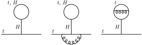
Figure 1: One- and two-loop tadpole contributions to the self-energy.

The renormalized self-energy of a massive fermion with pole mass $M$ in the on-shell scheme at one-loop order can be written as (we ignore complications arising from the Dirac structures involving $\gamma_{5}$)

$$\Sigma_{R}^{\rm OS}(p)=\Sigma_{0}(p)-\Sigma_{0}(p)\left.\right|_{p\!\!\!/=M}-M^{2}\frac{\partial\Sigma_{0}(p)}{\partial p^{2}}\left.\right|_{p\!\!\!/=M}\;,$$ (1)

where $\Sigma_{0}$ is the bare self-energy. One immediately finds that all momentum independent contributions, in particular those from tadpole-diagrams, cancel by construction. The same cancellation of momentum independent terms occurs at the two-loop level, where in (1) also mixed products of one-loop contributions have to be considered.

In the $\rm MS$ schemes one just subtracts the singular part of the Laurent expansion in $\varepsilon=(d-4)/2$ plus possibly some constant term specific for the scheme. In this case we have

$$\Sigma_{R}^{\rm MS}(p)=\Sigma_{0}(p)-\Sigma_{0}(p)_{\rm div+const}\;.$$ (2)

As a consequence, the prescription how to subtract constant terms does affect the definition of the MS-mass. One such constant contribution to $\Sigma_{0}$ arises from the Higgs tadpole diagrams (see Fig. 1). In [11, 12] these tadpole diagrams were included in the definition of the ${\rm MS}$-mass and their contribution remains present in the final result for the ${\rm MS}$-pole-mass relation. In contrast, throughout the calculation in [7, 8] the vanishing of the Higgs tadpole was used as one of the renormalization conditions (see e.g. [13] Eq. (3.4)). Therefore these tadpoles were absent in the definition of the ${\rm MS}$-mass and, correspondingly, in the evaluation of the diagrams relevant for the $\rho$-parameter, as required for a consistent result. (For early discussions of this issue at the one- and two-loop level see e.g. [14])

Since the strategy for the evaluation of the Feynman amplitudes is entirely different in [11, 12] compared to [7, 8] (expansions vs. closed analytic formulae), a comparison between the two results seems desirable. We therefore include the Higgs tadpole diagrams in the calculation of the ${\rm MS}$ top quark mass $m_{t,\rm tadp}$ based on [7, 8]. The impact of the tadpole diagrams shown in Fig. 1 is given by the ratio between $m_{t,\rm tadp}$ and $m_{t,\rm notadp}$ calculated for [7, 8]. In order $O(\alpha_{s}G_{F}^{2}m_{t}^{4})$ it reads

$$\frac{m_{t,\rm tadp}(\mu)}{m_{t,\rm notadp}(\mu)} = 1+X_{t}\left(-\frac{3}{2}\frac{M_{H}^{2}}{M_{t}^{2}}+4N_{c}\frac{M_{t}^{2}}{M_{H}^{2}}+\frac{3}{2}\frac{M_{H}^{2}}{M_{t}^{2}}\log\frac{M_{H}^{2}}{\mu^{2}}-4N_{c}\frac{M_{t}^{2}}{M_{H}^{2}}\log\frac{M_{t}^{2}}{\mu^{2}}\right)$$ (3)

$$+C_{F}\frac{\alpha_{s}}{4\pi}X_{t}\left(8N_{c}\frac{M_{t}^{2}}{M_{H}^{2}}\!+\!48N_{c}\frac{M_{t}^{2}}{M_{H}^{2}}\log\frac{M_{t}^{2}}{\mu^{2}}\!-\!24N_{c}\frac{M_{t}^{2}}{M_{H}^{2}}\log^{2}\frac{M_{t}^{2}}{\mu^{2}}\right),$$

where $M_{H}$ and $M_{t}$ are pole (on-shell) masses and the gaugeless limit has been employed.

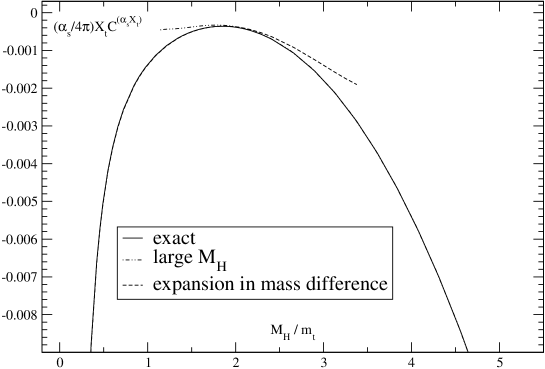
Figure 2: The two-loop coefficient $C^{(\alpha_{s}X_{t})}$ including the tadpole terms. The solid line represents the analytical result, the dashed line the expansion in the large $M_{H}$ limit, the dash-dotted line the expansion around $M_{H}=M_{t}$. All expansions are performed to fifth order.

Equation (3) can now be used to compare the two-loop relations between the $\overline{\rm MS}$ and the pole mass based on [11, 12] and [7, 8] respectively. This relation can be written as

$$\frac{m(\mu)}{M}=1+\frac{\alpha_{s}}{\pi}C^{(\alpha_{s})}+X_{t}C^{(X_{t})}+\frac{\alpha_{s}}{\pi}X_{t}C^{(\alpha_{s}X_{t})}+\dots,$$ (4)

$$X_{t}=\frac{G_{F}M_{t}^{2}}{8\sqrt{2}\pi^{2}}\approx 3\times 10^{-3}\,.$$ (5)

The coefficients $C^{(X_{t})}$ and $C^{(\alpha_{s}X_{t})}$ depend on the prescription. In the gaugeless limit they are functions of $M_{H}^{2}/M_{t}^{2}$ only.

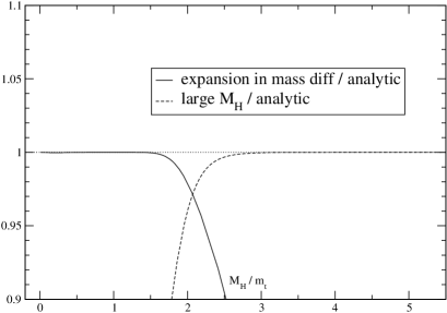
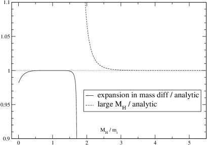
Figure 3: Ratio between expanded and analytic results in the scheme with (left figure) and without (right figure) tadpoles. The dashed line corresponds to the expansion in the large $M_{H}$ limit, the solid line to the expansion around $M_{H}=M_{t}$.

The result for the tadpole terms separately exhibits a power law behaviour in the limit $M_{H}^{2}/M_{t}^{2}\to 0$ and the limit $M_{t}^{2}/M_{H}^{2}\to 0$ whereas the complete result without tadpoles remains finite for $M_{H}^{2}/M_{t}^{2}\to 0$. Using Eq. (3) we find agreement between the results of [7, 8] and [11, 12]. This is demonstrated in Fig. 2 where we present the results for the two-loop coefficient $C^{(\alpha_{s}X_{t})}$ in the gaugeless limit employing the definition which includes the tadpole terms.

The corresponding ratios between the expanded and the analytic results are shown in Fig. 3 for both schemes (with and without tadpoles). From this comparison it is evident that the two calculations [7, 8] and [11, 12] do agree for the relation between pole- and $\overline{\rm MS}$-mass after compensating for the tadpole contributions, and that the expansion with five terms give an excellent approximation to the analytic result with less than 10% deviation at most and negligible deviation for the physically interesting range of the Higgs mass. In particular the agreement between the expansion around $M_{H}=M_{t}$ and the analytic result for small $M_{H}$ is remarkable, as already observed in [7].

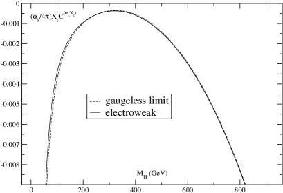
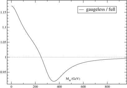
Figure 4: Comparison between $C^{(\alpha_{s}X_{t})}$ evaluated in the full electroweak theory and the gaugeless approximation. In the left figure, the solid line represents full electroweak theory, the dashed line the gaugeless limit. In the right figure, the ratio between the results in the full electroweak theory and the gaugeless limit for the two-loop coefficient $C^{(\alpha_{s}X_{t})}$ is shown.

It is also instructive to compare the result obtained in the gaugeless limit with the one [11] obtained in the full electroweak theory with nonvanishing $M_{W}$. In [12] it was shown that this difference is given by the following expression

$$\frac{\overline{m}^{\rm SM}_{t,\rm tadp}(M_{t})-\overline{m}^{\rm g.l.}_{t,\rm tadp}(M_{t})}{M_{t}~{}X_{t}}=-0.07978-0.429164\frac{\alpha_{s}}{4\pi}C_{f}$$

$$\qquad\qquad+\frac{M_{t}^{2}}{M_{H}^{2}}\left(1-4\frac{\alpha_{s}}{4\pi}C_{f}\right)\Biggl{[}-\frac{1}{2}\frac{M_{W}^{4}}{M_{t}^{4}}\left(1-3\ln\frac{M_{W}^{2}}{M_{t}^{2}}\right)-\frac{1}{4}\frac{M_{Z}^{4}}{M_{t}^{4}}\left(1-3\ln\frac{M_{Z}^{2}}{M_{t}^{2}}\right)\Biggr{]}\;.$$

The two-loop coefficients are compared in Fig. 4. The deviation is small and does not exceed 10% for $M_{H}>100$GeV.

Summary: The difference between [7, 8] and [11, 12] results from the exclusion of tadpole diagrams, which do not contribute to physical observables in the on-shell scheme. The results based on expansions around $M_{H}=M_{t}$ and the limit of large $M_{H}$ [7] are in perfect numerical agreement with the analytic results [11, 12]. The influence of non-zero $M_{W}$-mass terms is below 10% for $M_{H}>100$GeV, the region of interest for phenomenology.

Acknowledgments: The authors would like to thank K. Chetyrkin, M. Yu. Kalmykov, D. Kazakov, and F. Jegerlehner for helpful discussions and M. Yu. Kalmykov for providing the data in the full electroweak theory.

This work was supported by the Graduiertenkolleg “Hochenergiephysik und Teilchenastrophysik”, by BMBF under grant No. 05HT9VKB0, and the SFB/TR 9 (Computational Particle Physics).

References

- [1] D. A. Ross and M. J. G. Veltman, Nucl. Phys. B 95 (1975) 135.
- [2] M. J. G. Veltman, Nucl. Phys. B 123 (1977) 89.
-
[3]
A. Djouadi and C. Verzegnassi,
Phys. Lett. B 195 (1987) 265;
A. Djouadi, Nuovo Cim. A 100 (1988) 357. -
[4]
J. J. van der Bij and F. Hoogeveen,
Nucl. Phys. B 283 (1987) 477;
J. Fleischer, O. V. Tarasov, and F. Jegerlehner, Phys. Lett. B 319 (1993) 249. - [5] L. Avdeev et al., Phys. Lett. B 336 (1994) 560; [Erratum-ibid. B 349 (1995) 597].
- [6] K. G. Chetyrkin, J. H. Kuhn, and M. Steinhauser, Phys. Lett. B 351 (1995) 331.
- [7] M. Faisst et al., Nucl. Phys. B 665 (2003) 649.
- [8] J. J. van der Bij et al., Phys. Lett. B 498 (2001) 156.
- [9] M. Steinhauser, Comput. Phys. Commun. 134 (2001) 335.
- [10] T. Seidensticker, Diploma thesis (University of Karlsruhe, 1998), unpublished.
- [11] F. Jegerlehner and M. Y. Kalmykov, Nucl.Phys. B 676 (2004) 365.
- [12] F. Jegerlehner and M. Y. Kalmykov, Acta Phys. Pol. B 34 (2003) 5335.
- [13] A. Denner, Fortsch. Phys. 41 (1993) 307.
- [14] T. Appelquist et al., Phys. Rev. D 8 (1973) 1747; J. Fleischer and F. Jegerlehner, Phys. Rev. D 23 (1981) 2001; R. Hempfling and B. A. Kniehl, Phys. Rev. D 51 (1995) 1386.