Does HBT Measure the Freeze-out Source Distribution?

Abstract

It is generally assumed that as a result of multiple scattering, the source distribution measured in HBT interferometry corresponds to a chaotic source at freeze-out. This assumption is subject to question as effects of multiple scattering in HBT measurements must be investigated within a quantum-mechanical framework. Applying the Glauber multiple scattering theory at high energies and the optical model at lower energies, we find that multiple scattering leads to an effective HBT density distribution that depends on the initial chaotic source distribution with an absorption.

1 Introduction

Recent experimental measurements of HBT correlations in relativistic heavy-ion collisions show only relatively small changes of the extracted longitudinal and transverse radii as a function of collision energies, and the ratio of $R_{\rm out}/R_{\rm side}\sim 1$ [2]. The difficulties of explaining these HBT measurements with theoretical models, known as the “HBT puzzles”, have been discussed by many authors [3, 4]. In these comparisons with theoretical models, it is generally assumed that as a result of multiple scattering, the source distribution measured in an HBT measurement corresponds to a chaotic source at freeze-out, in which a detected hadron suffers its last hadron-hadron scattering.

In a recent quantum-mechanical treatment of the multiple scattering process using the Glauber theory at high energies and the optical model at lower energies, it was found that the HBT interferometry does not measure the freeze-out source distribution and the effective HBT density distribution depends on the initial chaotic source distribution with an absorption [5]. Effects of collective flows have also been investigated [5].

What is the physical basis for these new insights in HBT measurements? While the detailed arguments leading to the above results have been presented previously in Ref. [5], it is instructive to review here the most important features of the multiple scattering process and the HBT interferometry that give rise to the above unconventional viewpoints. We shall first examine the origin of the HBT interferometry in Section II and study next how the multiple scattering process will affect the HBT correlation function in Section III, using the quantum-mechanical Glauber theory of multiple scattering [6].

At the recent Quark Matter 2004 Conference, Kapusta and Li [7] reported new findings which support qualitatively some of the earlier results of Ref. [5].

2 HBT Interferometry for Chaotic Sources

We examine briefly the origin of the HBT correlation for identical bosons (pions), as reviewed in Chapter 17 of Ref. [8]. The HBT correlation is represented by the probability $P({k}_{1},{k}_{2})$ of detecting identical bosons with 4-momenta $k_{1}$ and $k_{2}$ in coincidence, or alternatively, by the correlation function $R({k}_{1},{k}_{2})$=$[P(k_{1},k_{2})/P({k}_{1})P({k}_{2})]$ -1 where $P(k)$ is the single-particle momentum distribution.

                              

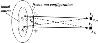
Figure 1: The shaded region represents the initial source which will
expand to the freeze-out configuration before the bosons reach the detectors.

$P(k_{1},k_{2})$ is given by squaring the total amplitude from all source points $(x_{1},x_{2})$,

$$P({k}_{1},{k}_{2})={1\over 2!}\bigl{|}\sum_{{x}_{1},{x}_{2}}A({k}_{1}{x}_{1})e^{i\phi_{0}({k}_{1}{x}_{1})}A({k}_{2}{x}_{2})e^{i\phi_{0}({k}_{2}{x}_{2})}\psi_{12}({x}_{1},{x}_{2})\bigr{|}^{2},$$ (1)

where $A({k}_{i}{x}_{i})$ and $\phi_{0}({k}_{i}{x}_{i})$ are the amplitude and the phase for the production of boson $k_{i}$ at the space-time point $x_{i}$ (Fig. 1). $\psi_{12}({x}_{1},{x}_{2})$ is the amplitude for the propagation of a pair of bosons $(k_{1},k_{2})$ from the source points $(x_{1},x_{2})$ to the detection points $(x_{d1},x_{d2})$,

$$\psi_{12}(x_{1},x_{2})={1\over\sqrt{2}}\biggl{\{}e^{{i{k}_{1}\cdot({x}_{d1}-{x}_{1})+i{k}_{2}\cdot({x}_{d2}-{x}_{2})}}+e^{{i{k}_{1}\cdot({x}_{d1}-{x}_{2})+i{k}_{2}\cdot({x}_{d2}-{x}_{1})}}\biggr{\}},$$ (2)

where the two terms represent amplitudes for two different histories of traveling from the source points to the detection points (the solid and the dashed trajectories (histories) of Fig. 1). If the source is coherent, there is no HBT correlation and $R({k}_{1},{k}_{2})=0$.

If the source is chaotic with random and fluctuating phases $\phi_{0}({k}{x})$, the absolute square of the sum in Eq. (1) becomes the sum of absolute squares,

$$P({k}_{1},{k}_{2})=\sum_{{x}_{1},{x}_{2}}A^{2}({k}_{1}{x}_{1})A^{2}({k}_{2}{x}_{2})|\psi_{12}({x}_{1},{x}_{2})|^{2}.$$ (3)

The HBT correlation is then present with a non-vanishing $R({k}_{1},{k}_{2})$. The correlation function $R(k_{1},k_{2})$ depends on the cross term of $|\psi_{12}(x_{1},x_{2})|^{2}$ of Eq. (2), which contains the phase difference between the two histories,

$${{k}_{1}\cdot({x}_{d1}-{x}_{1})+{k}_{2}\cdot({x}_{d2}-{x}_{2})}{-\left\{{k}_{1}\cdot({x}_{d1}-{x}_{2})+{k}_{2}\cdot({x}_{d2}-{x}_{1})\right\}}$$

$$=-({k}_{1}-{k}_{2})\cdot{x}_{1}-({k}_{2}-{k}_{1})\cdot{x}_{2}.$$ (4)

Representing $\sum_{x_{1}}$ by $\int d{x}_{1}\rho({x}_{1})$ with the source spatial density $\rho(x_{1})$, Eqs. (2)-(2) give

$$R({k}_{1},{k}_{2})\sim\left|~{}\,\int d{x}~{}~{}e^{-i({k}_{1}-{k}_{2})\cdot{x}}~{}~{}\rho_{\rm eff}(x;{k}_{1},{k}_{2})~{}\right|^{2},$$ (5)

$$\rho_{\rm eff}(x;{k}_{1},{k}_{2})={\rho({x})A({k}_{1},{x})A({k}_{2},{x})\over\sqrt{P({k}_{1})P({k}_{2})}}.$$ (6)

The measurement of $R(k_{1},k_{2})$ therefore provides information on the Fourier transform of the effective source distribution $\rho_{\rm eff}(x;{k}_{1},{k}_{2})$ of a chaotic source.

3 Multiple Scattering and HBT

In high-energy heavy-ion collisions, particles such as pions are produced and they will undergo multiple scattering until the system reaches the freeze-out configuration (Fig. 1). According to the Glauber theory of multiple scattering [6], the probability amplitude for a pion with momentum ${k}_{1}$ to go from the source point ${x}_{1}$ to the freeze-out point $x_{f1}$ and then to the detection point ${x}_{d1}$ is

$$\psi({x}_{1}\to{x}_{d1})=\exp\{i{k}_{1}\cdot({x}_{d1}-{x}_{1})+i\phi_{s}({x}_{f1}-{x}_{1})\}.$$ (7)

At high particle energies, the phase $\phi_{s}({x}_{f1}-{x}_{1})$ is the sum of two-body scattering phase shifts $\chi_{j}$ of the $N$ particles with which the particle scatters along its trajectory,

$$\phi_{s}({x_{f1}}-{x}_{1})=\sum_{j}^{N(x_{f1||}-x_{1||})}\chi_{j}(\hbox{\boldmath${x}$}_{1\perp}-\hbox{\boldmath${x}$}_{j\perp}),$$ (8)

where $x_{1||}$ and $\hbox{\boldmath${x}$}_{1\perp}$ are coordinates longitudinal and transverse to $\hbox{\boldmath${k}$}_{1}$. At lower energies, $\phi_{s}({x}_{f1}-{x}_{1})$ is given in terms of the two-body optical potential $V_{j}(\hbox{\boldmath${x}$}_{1}-\hbox{\boldmath${x}$}_{j})$ and the particle velocity $v$,

$$\phi_{s}({x}_{f1}-{x}_{1})=-\int_{x_{1\|}}^{{x_{f1\|}}}{1\over v}\sum_{j}^{N(x_{f1||}-x_{1||})}V_{j}({\tilde{\hbox{\boldmath${x}$}}}_{1}-{\hbox{\boldmath${x}$}}_{j})d{\tilde{x}}_{1\|}.$$ (9)

The probability amplitude (7) leads to the proper classical transport description of the particle in a medium [9]. It modifies the wave function $\psi_{12}(x_{1},x_{2})$ of Eq. (2) to

$$\psi_{12}(x_{1},x_{2})={1\over\sqrt{2}}\bigl{\{} e^{{i{k}_{1}\cdot({x}_{d1}-{x}_{1})+i\phi_{s}({x}_{f1}-{x}_{1})+i{k}_{2}\cdot({x}_{d2}-{x}_{2})+i\phi_{s}({x}_{f2}-{x}_{2})}}~{}~{}~{}~{}~{}~{}~{}~{}~{}~{}~{}~{}~{}$$ (10)

$$+ e^{{i{k}_{1}\cdot({x}_{d1}-{x}_{2})+i\phi_{s}({x}_{f2}^{\prime}-{x}_{2})+i{k}_{2}\cdot({x}_{d2}-{x}_{1})+i\phi_{s}({x}_{f1}^{\prime}-{x}_{1})}}~{}~{}~{}\bigr{\}},$$

where $({x}_{f1}{x}_{f2})$ and $({x}_{f1}^{\prime}{x}_{f2}^{\prime})$ are the two sets of freeze-out coordinates for the two histories (Fig. 1). In an HBT measurement of a chaotic source, the difference of the phases in the cross term of $|\psi_{12}(x_{1},x_{2})|^{2}$ in Eq. (2) is now modified to

$${~{}~{}~{}~{}{k}_{1}\cdot({x}_{d1}-{x}_{1})+\phi_{s}({x}_{f1}-{x}_{1})\,+{k}_{2}\cdot({x}_{d2}-{x}_{2})+\phi_{s}({x}_{f2}-{x}_{2})}$$

$${-\{{k}_{1}\cdot({x}_{d1}-{x}_{2})+\phi_{s}^{*}({x}_{f2}^{\prime}-{x}_{2})+{k}_{2}\cdot({x}_{d2}-{x}_{1})+\phi_{s}^{*}({x}_{f1}^{\prime}-{x}_{1})\}}$$

$$~{}~{}~{}~{}~{}\equiv-({k}_{1}-{k}_{2})\cdot{x}_{1}-({k}_{2}-{k}_{1})\cdot{x}_{2}+\Delta,$$ (11)

where we introduce $\Delta$ to represent the effects of multiple scattering. For the measurement of $R_{\rm out}$, $\hbox{\boldmath${k}$}_{1}-\hbox{\boldmath${k}$}_{2}$ is along $\hbox{\boldmath${k}$}_{1}$, we have $\hbox{\boldmath${x}$}_{f1}=\hbox{\boldmath${x}$}_{f1}^{\prime}{\rm~{}and~{}}\hbox{\boldmath${x}$}_{f2}=\hbox{\boldmath${x}$}_{f2}^{\prime}$,

$$\phi_{s}({x}_{f1}-{x}_{1})=\phi_{s}({x}_{f1}^{\prime}-{x}_{1}),{~{}~{}\rm and~{}~{}}\phi_{s}({x}_{f2}-{x}_{2})=\phi_{s}({x}_{f2}^{\prime}-{x}_{2}).$$ (12)

For the measurement of $R_{\rm side}$ and $R_{\rm long}$, $\hbox{\boldmath${k}$}_{1}-\hbox{\boldmath${k}$}_{2}=\hbox{\boldmath${q}$}$ is perpendicular to $\hbox{\boldmath${k}$}_{1}$, and

$$~{}~{}~{}~{}~{}~{}~{}~{}~{}~{}~{}{\cal R}e~{}\phi_{s}({x}_{f1}-{x}_{1})-{\cal R}e~{}\phi_{s}({x}_{f1}^{\prime}-{x}_{1}) = ({x}_{f1}-{x}_{f1}^{\prime})\cdot\nabla{\cal R}e~{}\phi_{s}({x}_{f1}-{x}_{1})$$ (13)

$$\propto ~{}~{}~{}\hbox{\boldmath${q}$}\cdot\nabla_{\perp}{\cal R}e~{}\phi_{s}({x}_{f1}-{x}_{1})~{}~{}\sim~{}0,$$

where the last approximate equality arises as the vector sum in $\nabla_{\perp}{\cal R}e~{}\phi_{s}$ with random transverse vector contributions from many independent scatterings is approximately zero. In both cases, the real parts of the phase differences cancel approximately, and only the imaginargy parts remain,

$$\Delta\sim 2i~{}{\cal I}m~{}\phi_{s}({x}_{f1}-{x}_{1})+2i~{}{\cal I}m~{}\phi_{s}({x}_{f2}-{x}_{2}).$$ (14)

From Eqs. (3) and (14), $R(k_{1},k_{2})$ is again given by Eq. (5) but the HBT effective density distribution $\rho_{\rm eff}(x;k_{1},k_{2})$ of Eq. (6) is modified, in the case of multiple scattering, to [5]

$$\rho_{\rm eff}(x;{k}_{1},{k}_{2})={e^{-2~{}{\cal I}{m}~{}\phi_{s}({x}_{f}-x)}\rho({x})A({k}_{1},{x})A({k}_{2},{x})\over\sqrt{P({k}_{1})P({k}_{2})}}\,.$$ (15)

The effective distribution depends on the initial source distribution with an absorption.

4 Conclusions and Discussions

Comparing the results of the last two sections, we see that the new insights concerning the multiple scattering process and HBT measurements arise from the following considerations: (1) In a quantum mechanical description, the multiple scattering process gives rise to the accumulation of phases along the trajectories of the detected particles. (2) For a chaotic source, the HBT correlation arises from the difference in the phases accumulated in two different sets of particle trajectories. (3) For these two sets of trajectories, the real parts of the accumulated phases due to the multiple scattering process approximately cancel each other and only the imaginary absorptive parts remain.

Based on these considerations, we find that the multiple scattering process leads to an effective density distribution that depends on the initial chaotic source distribution with an absorption, Eq. (15). The effects of the longitudinal momentum loss can be further included in the future by using the extension of the Glauber theory formulated by Blankenbecler and Drell [10]. While the absorption and the longitudinal momentum loss will modify the transmission of the initial chaotic source distribution, the effective source is closer to the initial chaotic source configuration and the nuclear geometrical overlap than the freeze-out configuration. As a consequence, the present new insights may pave the way for a better understanding of the HBT puzzles.

Acknowledgment

The author wishes to thank Profs. R. Blankenbecler, R. Glauber, and Weining Zhang for valuable discussions. This research was supported by the Division of Nuclear Physics, U.S. D.O.E., under Contract DE-AC05-00OR22725 managed by UT-Battelle, LLC.

References

References

- [1]
- [2] K. Adcox , PHENIX Collaboration, Phys. Rev. Lett. 88, 192302 (2002); C. Adler , STAR Collaboration, Phys. Rev. Lett. 87, 082302 (2001); M. Lisa , E895 Collaboration, Phys. Rev. Lett. 84, 2789 (2000); L. Ahle , E802 Collaboration, Phys. Rev. C66, 054906 (2002); M.M. Aggarwal , WA98 Collaboration, Eur. Phy. Jour. C16, 445 (2000).
- [3] U. A. Wiedemann, U. Heinz, Phys. Rept. 319 145 (1999); U. Heinz and P. Kolb, Nucl. Phys. A702, 269 (2002); D. Molnár and M. Gyulassy, nucl-th/0204062 and nucl-th/0211017.
- [4] S. Pratt, Nucl. Phy. A715, 389c (2003); D. Magestro, and H. Appelshauser, QM2004 Proceedings.
- [5] C. Y. Wong, J. Phys. G29, 2151 (2003), [nucl-th/0302053].
- [6] R. J. Glauber, in Lectures in Theoretical Physics, (Interscience, N.Y., 1959), Vol. 1, p. 315.
- [7] J. Kapusta and Yang Li, QM2004 Proceedings.
- [8] C. Y. Wong, Introduction to High-Energy Heavy-Ion Collisions, (World Scientific Publishing Company, 1994).
- [9] C. Y. Wong and R. Glauber, to be published.
- [10] R. Blankenbecler and S. Drell, Phys. Rev. D53, 6265 (1996).